Stock Index Return Volatility Forecast via Excitatory and Inhibitory Neuronal Synapse Unit with Modified MF-ADCCA

Abstract

Financial prediction persists a strenuous task in Fintech research. This paper introduces a multifractal asymmetric detrended cross-correlation analysis (MF-ADCCA)-based deep learning forecasting model to predict a succeeding day log return via excitatory and inhibitory neuronal synapse unit (EINS) using asymmetric Hurst exponent as input features, with return and volatility increment of Shanghai Stock Exchanges Composite Index (SSECI) from 2014 to 2020 as proxies for analysis. Experimental results revealed that multifractal elements by MF-ADCCA method as input features are applicable to time series forecasting in deep learning than multifractal detrended fluctuation analysis (MF-DFA) method. Further, the proposed biologically inspired EINS model achieved satisfactory performances in effectiveness and reliability in time series prediction compared with prevalent recurrent neural networks (RNNs) such as LSTM and GRU. The contributions of this paper are to (1) introduce a moving-window MF-ADCCA method to obtain asymmetric Hurst exponent sequences used directly as an input feature for deep learning prediction and (2) evaluate performances of various asymmetric multifractal approaches for deep learning time series forecasting.

1. Introduction

Financial trends fluctuations have amassed complexities by rapid global markets development in the recent decades. Time series prediction is a strenuous task since it contains chaotic, fuzzy, and incomplete information [1]. The focus of this paper is to interpret the financial fluctuation patterns and to predict their future trends.

Financial researchers often used statistical and econometric methods to construct prediction models by studying the characteristics and operating rules to assess and forecast volatility before the advent of machine learning algorithms. They indicated that financial market is a synthetical object with nonlinear multifractal characteristics [2,3], where multiscale properties and nonlinear evolution can be quantitatively analyzed by self-similar behavior of multifractal theory. These multifractal analysis techniques include rescaled range analysis (R/S) [4], detrended fluctuation analysis (DFA) [5], and multifractal detrended fluctuation analysis (MF-DFA) [6]. To compare, DFA can eliminate estimates of long-term relationships and increase credibility than rescaled range analysis, whereas multifractal detrended cross-correlation analysis (MF-DCCA) [7] is proposed to combine MF-DFA and DCCA [8] identifying the cross-correlation between two non-stationary data to quantify multifractal characteristics of the correlation. MF-DCCA method has extended to numerous research [9,10] such as multifractal asymmetric detrended cross-correlation analysis (MF-ADCCA) [11] studying asymmetric cross-correlations of non-stationary time series by integrating MF-DCCA with asymmetric DFA [12] to address its predicting upward (or downward) trend of cross-correlation characteristic limitation in time series. It studied the scaling features of cross-correlation between finance market stability and real estate price changes [13], in cryptocurrency markets research [14], and in gold futures market’s price-volume correlation [15] indicating that MF-ADCCA is effective to complex nonlinear dynamics.

The generalized Hurst exponent ($H$) is an econophysics concept to describe time series features and evaluate their complexities as a quantitative metric to study time series long-range dependence by various multifractal analysis approaches. A time series is characterized by anti-persistent behavior when $0<H<$ 0.5, which means that the data are uncorrelated temporally. In this case, the relative tendency shows the potential for an enormous reversal signal and continuity. When $0.5<H<$ 1, the relative tendency is characterized by persistent behavior, its current trend continuity is likely in time series contrary to the previous case. If $H$ = 0.5, the time series is expected to be neither anti-persistent nor persistent but is characterized by a negatively correlated dataset with any definable behavior. Hence, the generalized Hurst exponent is valuable for quantifying time series tendency.

Although asymmetric Hurst exponents can provide probabilistic trend assessments to express the likelihood of a continuous trend, but cannot provide a precise forecast of future values as they are sensitive to non-stationary or precipitous data changes in time series behaviors [16,17,18]. Deep learning methods for financial prediction has gradually become the core direction of fintech research in recent years [19,20]. Recurrent neural networks (RNNs) are mostly used time series prediction models for long-range time series dependence with their unique memory mechanisms to generate the current state by using the hidden state of previous time step as input to store past information [21]. Nevertheless, vanishing and exploding gradients problems occurred when the network parameters are trained repetitively in model training process inducing RNNs inability to guarantee generality and reliability of the prediction model. A biologically motivated recurrent unit based on neuronal synaptic activity mechanism and chaotic behaviors called excitatory and inhibitory neural synapse unit (EINS) is proposed by the author’s previous research to address these problems.

Additionally, a novel deep learning model is introduced to forecast absolute return of SXP500 Index by combining RNNs and asymmetric fractality exponent (A-MFDFA) to explore asymmetric multifractal elements [22]. Experimental results indicated that asymmetric Hurst exponents improved deep learning approaches for absolute return prediction accuracy and robustness in volatile financial markets, but A-MFDFA method only analyzed multifractal characteristics of single non-stationary time series inducing the loss of cross-correlation information in financial factors. MF-ADCCA is a comprehensive technique to consider asymmetric structure and multifractal scaling features between two time series to improve complex nonlinear financial dynamics understanding, which is more appropriate than A-MFDFA as an input feature in financial forecasting.

Hence, this paper focuses on predicting financial time series via EINS using asymmetric Hurst exponent based on MF-ADCCA. First, it used a moving-window method to modify MF-ADCCA so that times series of past $T$ days can obtain asymmetric Hurst exponent of the day. Second, MF-ADCCA is to estimate asymmetric multifractal features of cross-correlations between price fluctuations and realized volatility of Shanghai Stock Exchanges Composite Index (SSECI). Third, the succeeding day log return is predicted by EINS using asymmetric Hurst exponent based on MF-ADCCA and log return of past $T$ days as input. Then, the predictive capacities of MF-ADCCA are examined and compared with MF-DFA-based RNNs model (delete and to be mentioned in results section-Experimental results showed that MF-ADCCA predictive capacities outperformed MF-DFA in deep learning financial forecasting tasks, and EINS model achieved satisfactory performances for effectiveness and reliability in time series prediction compared to RNNs such as LSTM [23] and GRU [24]).

This paper is organized as follows: Section 2 introduces a moving-window MF-ADCCA method and EINS; Section 3 presents the financial time series analyzed by MF-ADCCA and deep learning forecasting experiment implementation; Section 4 discusses the experimental results followed by conclusion in Section 5.

2. Materials and Methods

2.1. Multifractal Asymmetric Detrended Cross-Correlation Analysis (MF-ADCCA)

This subsection introduces MF-ADCCA method used in time series prediction experiment to measure the asymmetric cross-correlations between two non-stationary time series $\left\{x_t:t=1,\dots .,N \right\}$ and $\left\{y_t:t=1,\dots .,N \right\}$, and examine the aggregated index to present a positive or a negative increment [11] summarized as follows:

Step 1: Construct profile of the original time series as

$$X(k)={\displaystyle \sum _{t=1}^k(x_t-\overline{x}),t=1,\dots ,N,}$$

(1)

$$Y(k)={\displaystyle \sum _{t=1}^k(y_t-\overline{y}),t=1,\dots ,N,}$$

(2)

where $\overline{x}$ and $\overline{y}$ are average values over the entire return series respectively. The index proxy series is calculated by $I\left(k\right)=I\left(k-1\right)\exp \left(x_k\right) \mathrm{for} k=1,\dots ,N$ with $I\left(0\right)=1$ to assess positive and negative trend of the index.

Step 2: Divide profiles $X\left(k\right)$, $Y\left(k\right)$, and index proxy $I\left(k\right)$ into $N_S=\lfloor N/s\rfloor$ non-overlapping segments of length $s$. Repeat the division from other end of the series to consider the whole profile for a total of $2N_S$ segments for each series.

Step 3: Calculate detrended covariance for each $2N_S$ segment as

$$f^2(s,v)=\frac{1}{s}{\displaystyle \sum _{i=1}^s|X((v-1)s+i)-\widetilde{X_v}(i)||Y((v-1)s+i)-{\tilde{Y}}_v(i)|}$$

(3)

for $v=1,\dots ,N$, and

$$f^2(s,v)=\frac{1}{s}{\displaystyle \sum _{i=1}^s|X(N-(v-N_s)s+i)-{\tilde{X}}_v(i)||Y(N-(v-N_s)s+i)-{\tilde{Y}}_v(i)|}$$

(4)

for $v=1,\dots ,2N_S$. By fitting a least-square degree-2 polynomial ${\tilde{X}}_v \mathrm{and} {\tilde{Y}}_v$, calculate profiles local trend and applied to detrend $X\left(k\right)$ and $Y\left(k\right)$ respectively. Further, the local asymmetric direction of the index is determined by assessing the least-square linear fit ${\tilde{I}}_v\left(i\right)=a_{I_v}+b_{I_v}i\left(i=1,\dots ,s\right)$ for each segment, where the sign of slope $b_{I_v}$ is to discriminate the index trend. If $b_{I_v}>0$, the index trend has a positive trend, or a negative trend if otherwise.

Step 4: Calculate directional $q$-order average fluctuation functions as

$$\begin{array}{c}{F}_q^{+}(s)|={\left\{\frac{1}{M^{+}}{\displaystyle \sum _{v=1}^{2N_s}\frac{1+\mathrm{sgn}(b_{I_v})}{2}{\left[f^2(s,v)\right]}^{q/2}}\right\}}^{1/q},\\ F_q^{-}(s)|={\left\{\frac{1}{M^{-}}{\displaystyle \sum _{v=1}^{2N_s}\frac{1-\mathrm{sgn}(b_{I_v})}{2}{\left[f^2(s,v)\right]}^{q/2}}\right\}}^{1/q},\end{array}q\ne 0$$

(5)

and

$$\begin{array}{c}{F}_0^{+}(s)=\exp \left\{\frac{1}{2M^{+}}{\displaystyle \sum _{v=1}^{2N_s}\frac{1+\mathrm{sgn}(b_{I_v})}{2}\mathrm{In}\left[f^2(s,v)\right]}\right\},\\ F_0^{-}(s)=\exp \left\{\frac{1}{2M^{-}}{\displaystyle \sum _{v=1}^{2N_s}\frac{1-\mathrm{sgn}(b_{I_v})}{2}\mathrm{In}\left[f^2(s,v)\right]}\right\},\end{array}q=0$$

(6)

where $M^{+}={\displaystyle {\sum }_{v=1}^{2N_s}\frac{1+\mathrm{sgn}{b}_{(I_v)}}{2}}$ and $M^{-}={\displaystyle {\sum }_{v=1}^{2N_s}\frac{1+\mathrm{sgn}{b}_{(I_v)}}{2}}$ are subseries numbers with positive and negative tendencies in which $b_{I_v} \ne$ 0 for $v=1,\dots ,2N_S,$ thus $M^{+}+M^{-}=2N_S$.

Step 5: Calculate $q$-order fluctuation functions for overall trend as

$$F_q(s)={\left\{\frac{1}{2N_s}{\displaystyle \sum _{v=1}^{2N_s}{\left[f^2(s,v)\right]}^{\frac{q}{2}}}\right\}}^{\frac{1}{q}},q=0$$

(7)

and

$$F_0(s)=\exp \left\{\frac{1}{4N_s}{\displaystyle \sum _{v=1}^{2N_s}\mathrm{In}\left[f^2(s,v)\right]}\right\},q\ne 0$$

(8)

Step 6: Calculate generalized Hurst exponents as

$$F_q^{+}\left(s\right)\sim s^{h_{xy}^{+}\left(q\right)},F_q^{-}\left(s\right)\sim s^{h_{xy}^{-}\left(q\right)}, \mathrm{and} F_q\left(s\right)\sim s^{h_{xy}\left(q\right)}$$

(9)

when $q$-order fluctuation functions follow a power-law of forms $F_q^{+}\left(s\right)\sim s^{h_{xy}^{+}\left(q\right)},F_q^{-}\left(s\right)\sim s^{h_{xy}^{-}\left(q\right)}, \mathrm{and} F_q\left(s\right)\sim s^{h_{xy}\left(q\right)}$, the two non-stationary series present long-range power-law cross-correlated features. Scaling exponent $h_{xy}\left(q\right)$, known as generalized Hurst exponent, is used to express the long-range power-law correlation features that can be calculated by fitting a log-log linear regression, while $h_{xy}^{+}\left(q\right) \mathrm{and} h_{xy}^{-}\left(q\right)$ are used to measure the positive and negative increments. To avoid errors and preserve estimation validity, this paper used a scale range from $s_{min}=max\left(20,N/100\right) \mathrm{to} s_{max}=min\left(20s_{min},N/10\right)$ and 100 points in the regression [14].

If $0<h_{xy}\left(q\right)<0.5$, the two series present an anti-persistent cross-correlation indicating that one series is likely to be followed by a fluctuation opposite to the current trend in the other series. If $0.5<h_{xy}\left(q\right)<1$, the two series present persistent cross-correlation indicating that one series is likely to be followed by a fluctuation similar to the current trend in the other series. When $h_{xy}\left(q\right)$ = 0.5, the two series have neither obvious cross-correlations nor any correlation.

The order $q$ represents to various volatility magnitudes degree assessed. If $0<q$, scaling exponents present larger or smaller fluctuations behavior. Additionally, if $h_{xy}\left(q\right)$ is independent of $q$, a series is multifractal. It is noted that the Hurst exponent of target series can be calculated by setting $q$ = 2. Since the generalized Hurst exponents series calculated by MF-ADCCA cannot be used directly as input feature for deep learning forecasting, a moving-window method is used to modify MF-ADCCA by calculating asymmetric Hurst exponent value of the day using past $T$ days data depicted in Algorithm 1.

Algorithm 1. Algorithm to Moving-window MF-ADCCA Method.
Input:    Time Series: $X_t$;		< Size ($w\ast l$) >
Time Series: $Y_t$;		< Size ($w\ast l$) >
Days Scaling: $T$;
Step: $t$;
Output:   Asymmetric generalized Hurst exponents;
Function Moving-window MF-ADCCA ($X_t, Y_t, T, t$)
Initialize $\mathit{H}\mathit{u}\mathit{r}\mathit{s}\mathit{t}\leftarrow A$rray[0,…$N_{w-T+1}$]$, \mathit{H}\mathit{u}\mathit{r}\mathit{s}{\mathit{t}}^{+}\leftarrow A$rray[0,…$N_{w-T+1}$],       $\mathit{H}\mathit{u}\mathit{r}\mathit{s}{\mathit{t}}^{-}\leftarrow A$rray[0,…$N_{w-T+1}$]
for $i$ in range (0, $N_{w-T+1}$, step) do
$Series A\leftarrow X_t\left[i,\dots i+T\right]$        $Series B\leftarrow Y_t\left[i,\dots i+T\right]$
$\mathit{H}\mathit{u}\mathit{r}\mathit{s}\mathit{t}, , \mathit{H}\mathit{u}\mathit{r}\mathit{s}{\mathit{t}}^{+}, \mathit{H}\mathit{u}\mathit{r}\mathit{s}{\mathit{t}}^{-}\leftarrow MF-ADCCA\left(Series A, Series B\right)$
$\mathit{H}\mathit{u}\mathit{r}\mathit{s}{\mathit{t}}_{\left[\mathit{i}\right]} \leftarrow \mathit{H}\mathit{u}\mathit{r}\mathit{s}\mathit{t}$
$\mathit{H}\mathit{u}\mathit{r}\mathit{s}{\mathit{t}}_{\left[i\right]}^{+} \leftarrow \mathit{H}\mathit{u}\mathit{r}\mathit{s}{\mathit{t}}^{+}$
$\mathit{H}\mathit{u}\mathit{r}\mathit{s}{\mathit{t}}_{\left[\mathit{i}\right]}^{-}\leftarrow \mathit{H}\mathit{u}\mathit{r}\mathit{s}{\mathit{t}}^{-}$
return  $\mathit{H}\mathit{u}\mathit{r}\mathit{s}\mathit{t}, , \mathit{H}\mathit{u}\mathit{r}\mathit{s}{\mathit{t}}^{+}, \mathit{H}\mathit{u}\mathit{r}\mathit{s}{\mathit{t}}^{-}$
End function

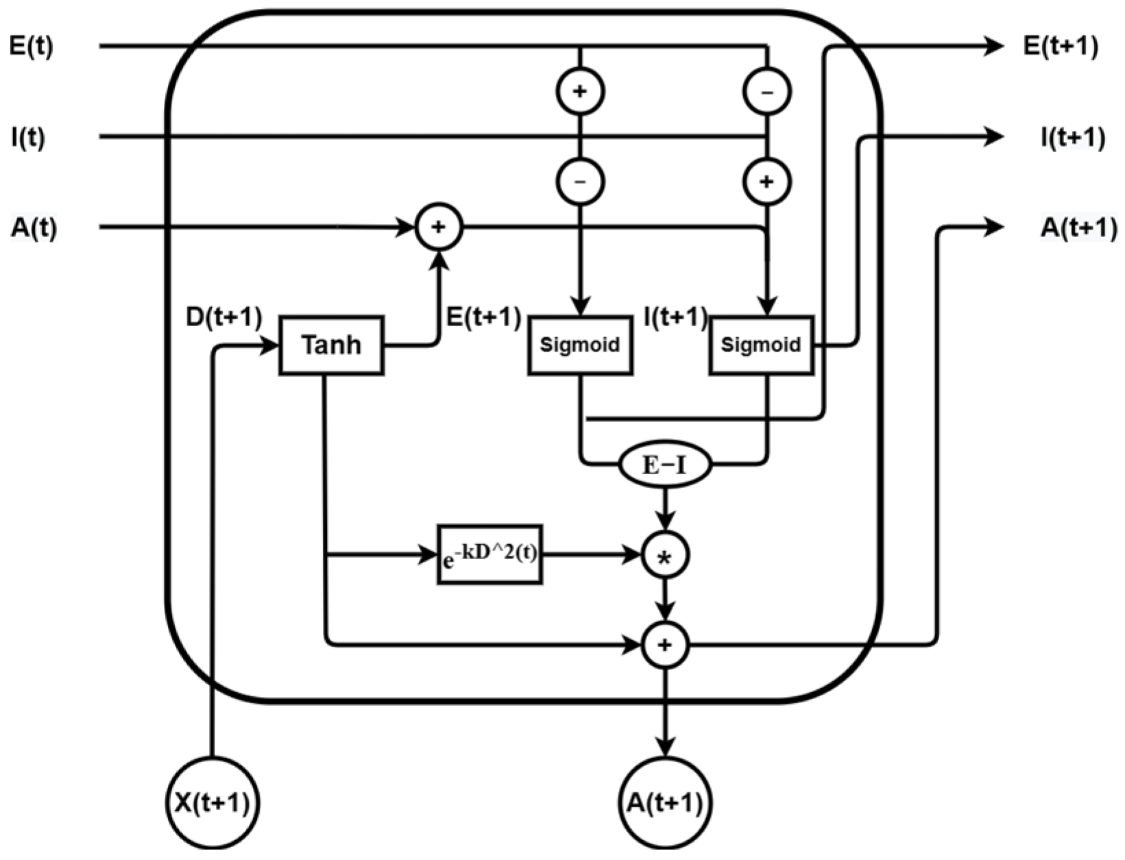
2.2. Excitatory and Inhibitory Neuronal Synapse Unit (EINS)

This section explains an EINS illustrated in Figure 1. It is a biologically inspired neural network model with synaptic activity mechanism to simulate the neurodynamics of spike alternation and neurotransmitter transmission within neurons during memory behavior [25,26,27]. The design is based on memristive synapse-coupled bi-neuron networks structure enabling the model to have the same memory mechanisms as human brain [28,29,30]. A single EINS unit is expressed as follows:

$$D\left(t+1\right)=Tanh \left[x\left(t+1\right)Wd-Bd \right]$$

(10)

$$E\left(t+1\right)=Sigmoid\left[A\left(t\right)\left.Wea+E\left(t\right)Wee-I\left(t\right)Wei+D\left(t+1\right)Wed-B_e\right]\right.$$

(11)

$$I\left(t+1\right)=Sigmoid\left[A\left(t\right)\left.Wia-E\left(t\right)Wie+I\left(t\right)Wii+D\left(t+1\right)Wid-B_i\right]\right.$$

(12)

$$A\left(t+1\right)=\left[E\left(t+1\right)-I\left(t+1\right)\right]e^{-k{D}^2\left(t+1\right)}+D\left(t+1\right)$$

(13)

where x(t+1) denotes the external stimulation at each time step; $D\left(t+1\right)$, $E\left(t+1\right)$, $I\left(t+1\right)$, $A\left(t+1\right)$ denote the neuronal dendrite layer, excitatory neurotransmitter state layer, inhibitory neurotransmitter state layer, and the neuronal axon layer, respectively; $Wea$, $Wee$, $Wei$, $Wed$, and $B_e$ express weights and bias of neuronal axon, excitatory neurotransmitter state, inhibitory neurotransmitter state, neuronal dendrite, and excitatory state layer in the excitatory state layer $E\left(t+1\right)$ respectively; similarly, $Wia$, $Wie$, $Wii$, $Wid$, and $B_i$ are weights and bias of corresponding terms in the inhibitory state layer, $I\left(t+1\right)$.

It showed that the dendrite layer receives external input and sends processed results to the hidden state with previous state values. The updated hidden state values are preserved in the hidden state to be learnt in subsequent time steps. Further, the proposed unit outputs the learnt result via an axon layer using the neurodynamic mechanism of memristive synapse-coupled bi-neuron networks and sends it to the next hidden state. Its model is depicted in Algorithm 2.

Algorithm 2. Algorithm to Excitatory and Inhibitory Neural Synapse Model.
Input:    Time Series: $T_t$;	< Size ($batch,time step, input size$) >
Input Size: $I$; Hidden Size: $H$; Output Size: $O$;
Step: $t$;
Output:   Prediction Result: $T_{t+1}$;
Procedure EINS ($n, p, i, j,{\theta }_0$)
Initialize ${\mathit{E}}_{\mathit{t}}\leftarrow$0; ${\mathit{I}}_{\mathit{t}}\leftarrow 0$; ${\mathit{A}}_{\mathit{t}}\leftarrow 0$; $\theta \leftarrow {\theta }_0$; $i\leftarrow 0$; $j\leftarrow 0$.
for $X_i$ in $T_t$ do
${\mathit{D}}_{\mathit{t}}\leftarrow tanh\left(X_i{W}_d^{I\ast H}-b_d^H\right)$        ${\mathit{E}}_{\mathit{t}}\leftarrow \delta \left(A_{t-1}{W}_{ea}^{H\ast H}+E_{t-1}{W}_{ee}^{H\ast H}-I_{t-1}{W}_{ei}^{H\ast H}+D_t{W}_{ed}^{H\ast H}-b_e^H\right)$
${\mathit{I}}_{\mathit{t}}\leftarrow \delta \left(A_{t-1}{W}_{ia}^{H\ast H}-E_{t-1}{W}_{ie}^{H\ast H}+I_{t-1}{W}_{ii}^{H\ast H}+D_t{W}_{id}^{H\ast H}-b_i^H\right)$
${\mathit{A}}_{\mathit{t}}\leftarrow \left(E_t-I_t\right)\odot ex{p}^{-k\ast D_t^2}+D_t$        $T_{t+1}\leftarrow \left(A_t{W}_O^{H\ast O}-b_O^O\right)$       return $T_{t+1}$
End for
While $j<p$ do
Update $\theta$ by running training algorithm for $n$ steps
$i\leftarrow i+n$
$T_{t+1}\leftarrow ValidationSetError\left(\theta \right)$
if $T_{t+1}<T_{valid}$ then
$j\leftarrow 0$
${\theta }^{\ast }\leftarrow \theta$
$i^{\ast }\leftarrow i$
else
$j\leftarrow j+1$
End if
End while
return ${\theta }^{\ast }$ and save the trained EINS model weights
End Procedure

RNNs memory mechanisms rely on preserving past information in hidden layer, their training encounters vanishing and exploding gradients problems occurred due to these trainable parameters are repetitively applied to the hidden state. The proposed experimental model used chaotic property of memristive synapse-coupled bi-neuron networks to mitigate them and explore the feasibility of combining biologically inspired approach with deep learning algorithms.

3. Data and Experiments

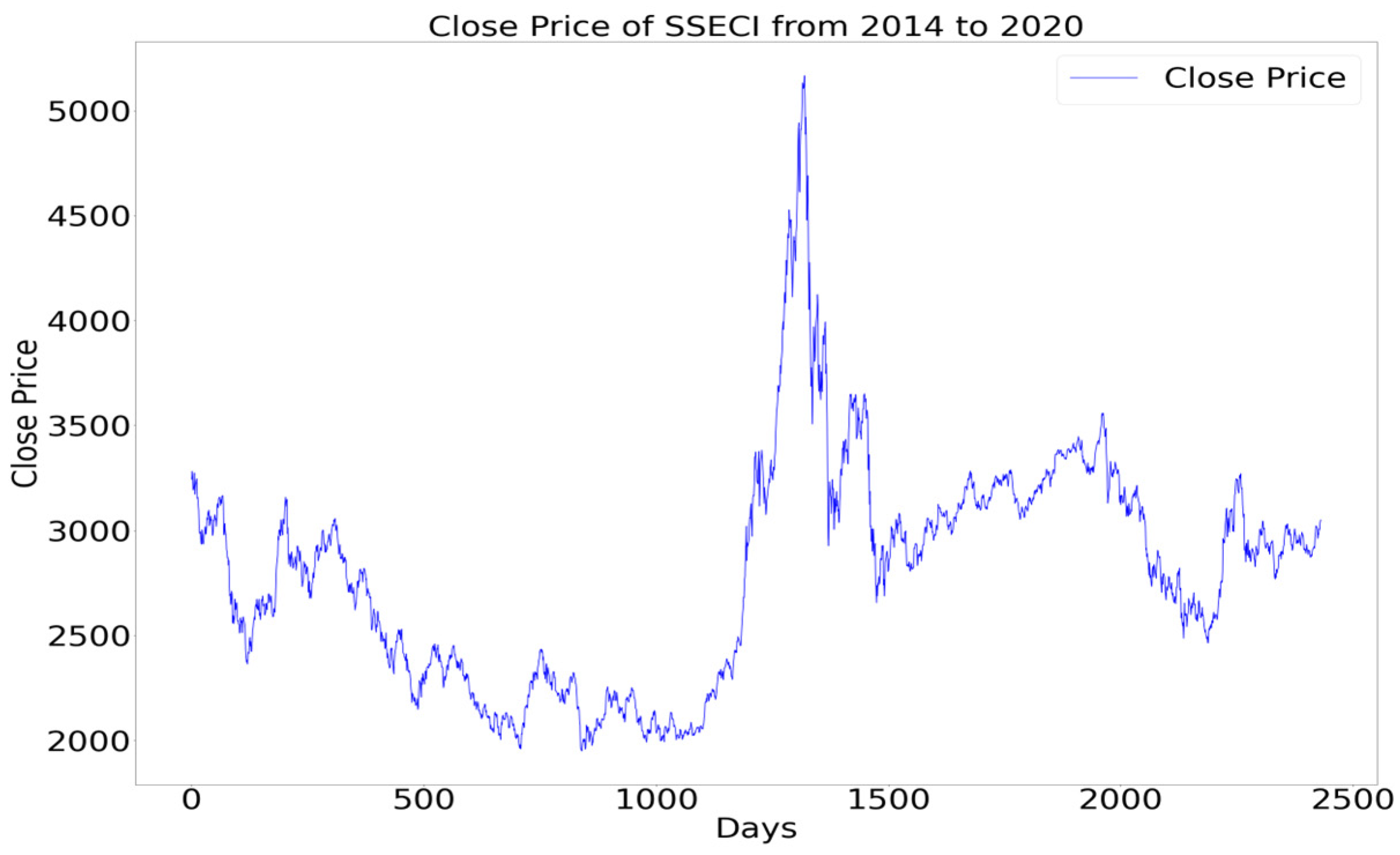
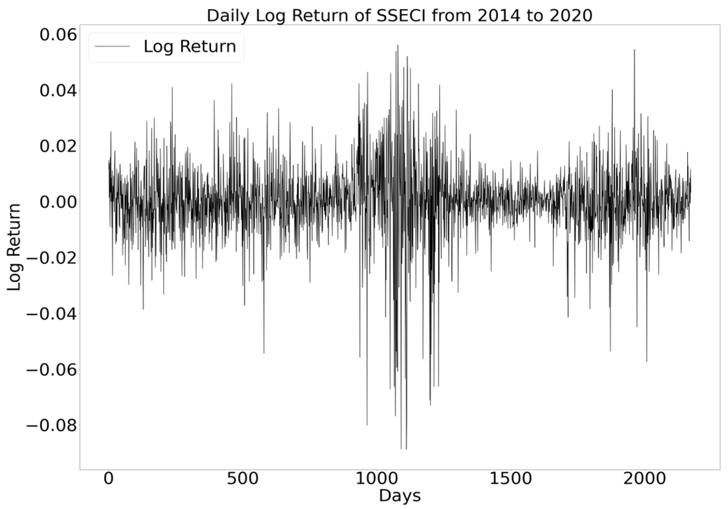
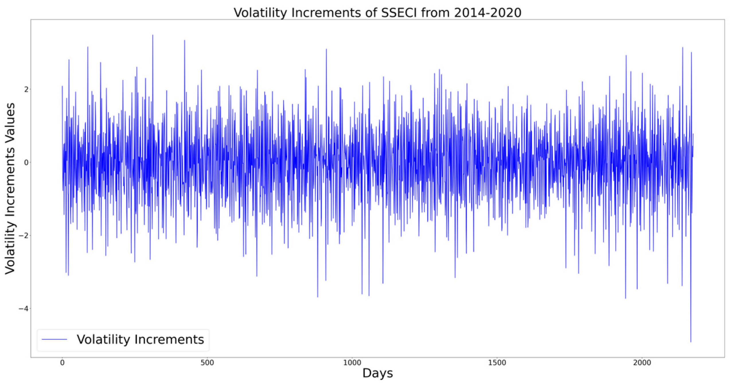
3.1. Data Description

The data are a log return series extracted by Shanghai Stock Exchanges Composite Index (SSECI). The experiment introduced a deep learning forecasting model with asymmetric multifractal characteristics, using close prices from 2014 to 2020 for calculation as depicted in Figure 2. The log return $r_t$ is calculated by:

$$r_t=\ln p_t-\ln p_{t-1}$$

(14)

where $p_t$ is daily close price on day $t$; $r_t$ is the log return on day $t$. The log return series of SSECI from 2014–2020 is illustrated in Figure 3. Additionally, the volatility increments from this period are another proxy for MF-ADCCA analysis given by:

$$v_t=\ln {\widehat{\sigma }}_t-\ln {\widehat{\sigma }}_{t-1}$$

(15)

where ${\widehat{\sigma }}_t=\sqrt{{\mathrm{BPV}}_t}$, and ${\mathrm{BPV}}_t$ represent the realized bipower variation [31] given by:

$${\mathrm{BRV}}_t={\displaystyle \sum _t\left|r_t\right|}\left|r_{t+1}\right|$$

(16)

Figure 4 illustrated the volatility increments (volatility changes) of SSECI. The data length of volatility increments series is 2177 similar to log return series. Augmented Dickey–Fuller (ADF) test [32], Kwiatkowski–Philips–Schmidt–Shin (KPSS) test [33], and Jarque-Bera statistic tests are implemented to examine statistical characteristics of two proxy series. The descriptive statistics information of the log return and volatility increments of SSECI are listed in

Table 1. Descriptive statistics for log return and volatility increments of SSECI.

	Mean	Max	Min	Std	Skew	Kurt	J-Bera 1	ADF 2	KPSS 3
$r_t$	$4.6\times {10}^{-5}$	$5.6\times {10}^{-3}$	$-8.9\times {10}^{-2}$	$1.3\times {10}^{-2}$	−0.953	6.695	4372.8 *	−9.148 *	$8.27\times {10}^{-2}$ *
$v_t$	$2.1\times {10}^{-4}$	3.7987	−3.7436	0.8384	$7.8\times {10}^{-3}$	1.0185	93.18 *	−15.769 *	$7.88\times {10}^{-2}$ *

¹ denotes Jarque-Bera statistic tests; ² denotes Augmented Dickey–Fuller test; ³ denotes Kwiatkowski–Philips–Schmidt–Shin (KPSS) test; * represents 1% significance level. Note: (1) The ADF test uses null to express the existence of a unit root; (2) the KPSS test uses the null to express stationary.

. It showed that the mean values of return increments and volatility increments are close to 0 indicating that these series are self-regression equilibrium. The absolute value of return increments is larger than volatility increments indicating that the return increments have greater asymmetry. Further, Jarque-Bera statistic test result showed that all series are not null hypothesis of Gaussian distribution at 1% significance level. It is noted that the null hypothesis of unit root existence in ADF test is rejected at 1% significance level, and KPSS tests showed that the null hypothesis of stationarity is rejected at 1% significance level.

The log return series and volatility increment series are used as proxies for MF-ADCCA analysis. Figure 5 and Figure 6 illustrated up-trend Hurst exponents ($h_{xy}^{+}\left(2\right)$) and up-trend Hurst exponents ($h_{xy}^{-}\left(2\right)$) of SSECI log returns based on the moving-window of MF-ADCCA analysis accordingly.

3.2. Experiments

The succeeding day log return of SSECI using past days log return with asymmetric Hurst exponents for experiment implementation are illustrated in Figure 7. The implementation code is written in Python 3.9 using Pytorch library on a hardware environment with Intel CPU Xeon@2.00 GHz, GPU Tesla V100, 12 GB RAM, and Windows 11 operating system. First, a moving-window MF-ADCCA is used to estimate the asymmetric Hurst exponent of Shanghai Stock Exchanges Composite Index (SSECI) and log return series volatility increments series are used as proxies. Second, the succeeding day log return of SSECI is predicted by EINS using asymmetric Hurst exponent based on the moving-window MF-ADCCA. Third, RNNs predictive capacities with MF-ADCCA are examined and compared with MF-DFA-based RNNs model such as LSTM and GRU. All datasets are normalized to the range from −1 to 1 with Min-Max normalized method prior feeding into the network as expressed by:

$$y_i=\frac{x_i-x_{mean}}{\underset{1\le i\le n}{max}\left\{x_j\right\}-\underset{1\le i\le n}{min}\left\{x_j\right\}}$$

(17)

where $y_i$ is the normalized value, $x_i$ is a data in the dataset, $x_{mean}$ is the mean value of sample set, $\underset{1\le i\le n}{max}\left\{x_j\right\}$ is the minimum data while $\underset{1\le i\le n}{min}\left\{x_j\right\}$ is the maximal data in the dataset. Each dataset is divided into three parts with the same train-valid-test split rate—80% is used for models’ training, 10% for validation, and the remaining for performance testing.

The experiment used a four-layer deep learning model structure for time series forecast two recurrent layers connected by two fully connected layers as illustrated in Figure 8, and used hyper-parameters to examine RNNs predictive capacities with MF-ADCCA as listed in

Table 2. Hyper-parameters setting list.

Hyper-Parameters	Settings
Hidden neurons	128,256
Time Horizons	32,128
Learning rate	$1\times {10}^{-3}$
Dropout rate	0.2
Epochs	100
Optimizer	Adam
Error function	Mean squared error

. Further, three regression indicators including mean square error ($MSE$), mean absolute error ($MAE$), and coefficient of determination ($R^2$) are used to evaluate models’ performances as given by:

$$MSE=\frac{1}{N}{\displaystyle \sum _{i=1}^N{({\tilde{y}}_t^i-y_t^i)}^2}$$

(18)

$$MAE=\frac{1}{N}{\displaystyle \sum _{i=1}^N\left|{\tilde{y}}_t^i-{\tilde{y}}_t^i\right|}$$

(19)

$$R^2=1-\frac{{\sum }_{i=1}^N\left(y_t^i-{\tilde{y}}_t^i\right))}{{\sum }_{i=1}^N\left({\overline{y}}_t^i-{\tilde{y}}_t^i\right)}$$

(20)

where $y_t^i$, ${\overline{y}}_t^i$, and ${\tilde{y}}_t^i$ represent the actual, the mean, and the predicted value of test set respectively; $N$ is the total samples number indicating that the lower $MSE$ and $MAE$ values represent more accurate prediction results. Further, the closer $R^2$ value to 1 represent the model robustness to fit dataset and prediction performance.

4. Results and Discussion

The experimental forecast results are listed in

Table 3. Forecasting performance with various hyper-parameters (note: best results highlighted in BOLD).

Multifractal	Model	MSE	MAE	${\mathit{R}}^2$
$\mathrm{Hidden} \mathrm{neurons}=128, \mathrm{Time} \mathrm{horizons}=32, \mathrm{Learning} \mathrm{rate}=1\times {10}^{-3}$
MF-DFA	EINS	0.02584	0.11069	−0.01746
	LSTM	0.02704	0.11351	−0.06485
	GRU	0.02769	0.11494	−0.09042
MF-ADCCA	EINS	0.02549	0.10999	−0.00398
	LSTM	0.02577	0.11091	−0.01469
	GRU	0.02580	0.11130	−0.01605
$\mathrm{Hidden} \mathrm{neurons}=128, \mathrm{Time} \mathrm{Horizons}=128, \mathrm{Learning} \mathrm{rate}=1\times {10}^{-3}$
MF-DFA	EINS	0.02324	0.10689	−0.00691
	LSTM	0.02337	0.10810	−0.01262
	GRU	0.02354	0.10885	−0.02011
MF-ADCCA	EINS	0.02372	0.10770	−0.02798
	LSTM	0.02507	0.11252	−0.08636
	GRU	0.02496	0.11118	−0.08178
$\mathrm{Hidden} \mathrm{neurons}=256, \mathrm{Time} \mathrm{Horizons}=32, \mathrm{Learning} \mathrm{rate}=1\times {10}^{-3}$
MF-DFA	EINS	0.02582	0.11069	−0.01666
	LSTM	0.02727	0.11501	−0.07390
	GRU	0.02699	0.11419	−0.06298
MF-ADCCA	EINS	0.02532	0.11003	0.00296
	LSTM	0.02704	0.11489	−0.06500
	GRU	0.02593	0.11145	−0.02102
$\mathrm{Hidden} \mathrm{neurons}=256, \mathrm{Time} \mathrm{Horizons}=128, \mathrm{Learning} \mathrm{rate}=1\times {10}^{-3}$
MF-DFA	EINS	0.02366	0.10756	−0.02516
	LSTM	0.02467	0.11103	−0.06923
	GRU	0.02774	0.11885	−0.20226
MF-ADCCA	EINS	0.02335	0.10705	−0.01197
	LSTM	0.02419	0.10989	−0.04810
	GRU	0.02418	0.11025	−0.04761

. They showed that MF-DFA asymmetric Hurst exponents achieved predictive capacities for forecasting time series with RNNs [19]. In particular, the performance of up-trend Hurst exponents ($h_{xy}^{+}\left(2\right)$) and up-trend Hurst exponents ($h_{xy}^{-}\left(2\right)$) for deep learning forecasting outperformed the generalized Hurst exponent ($h_{xy}\left(2\right)$). They are used as benchmarks to compare with MF-ADCCA asymmetric Hurst exponents to examine predictive capacities of various asymmetric multifractal analysis approaches.

They also showed that three evaluation metrics values MSE, MAE, and R² of MF-ADCCA-based forecasting models outperformed MF-DFA under corresponding hyper-parameters. However, the multifractal elements obtained by MF-ADCCA method lacked stability when fitted into deep learning model due to proxy design diversities. Hence, it is recommended to use indicators related to financial technical analysis as proxies for MF-ADCCA method since prerequisite fintech knowledge is essential. It is noted that the improvement in MF-ADCCA performance to multiple proxies mechanism allowed to retain more time series’ past information indicating that asymmetric multifractal elements by MF-ADCCA method as input features are applicable to time series forecasting in deep learning.

For deep neural network prediction performance, it examined the feasibility of combining neuroscience and brain science into deep learning algorithms. The results showed that EINS prediction error is lower than LSTM and GRU under corresponding hyper-parameters as its architecture and information flow are based on memristive synapse-coupled bi-neuron networks to simulate synapse activity mechanisms during electric signals exchange and chemical transmitters between neurons. It has a deep neural network model with neurodynamics of spike alternation and neuro-transmitter transmission within neurons during memory indicating that EINS is a significant comparison method for effectiveness and reliability in time series prediction.

5. Conclusions

This paper focused not only on predicting financial time series via EINS with asymmetric Hurst exponent based on MF-ADCCA, but also examined the predictive capacities of various asymmetric multifractal approaches in deep learning. The log return and volatility increment of Shanghai Stock Exchanges Composite Index (SSECI) from 2014 to 2020 are used as proxies for MF-ADCCA analysis. It used a moving-window MF-ADCCA to estimate the asymmetric Hurst exponent, and a succeeding day log return predicted by EINS using asymmetric Hurst exponent based on moving-window MF-ADCCA with log return of past $T$ days as input to examine MF-ADCCA predictive capacity in deep learning to compare with MF-DFA-based RNNs model. A four-layer deep learning model structure is constructed for time series forecast where two recurrent layers are connected by two fully connected layers. Further, mean square error (MSE), mean absolute error (MAE), and coefficient of determination ($R^2$) are used to evaluate the models’ performances. The results showed that MF-ADCCA outperformed MF-DFA in deep learning financial forecasting tasks. Further, the biologically inspired EINS model achieved satisfactory performances for effectiveness and reliability in time series prediction as compared with prevalent RNNs such as LSTM and GRU.

The contributions of this paper are to (1) introduce a moving-window MF-ADCCA method to calculate asymmetric Hurst exponent of the day using times series of the past $T$ days by setting $q$ = 2 to obtain asymmetric Hurst exponent sequences that can be directly used as an input feature for deep learning prediction and (2) evaluate various asymmetric multifractal approaches performances for deep learning time series forecasting.

Future research will focus on other financial markets such as cryptocurrency markets, gold markets, and other state-of-the-art multifractal methods as benchmarks.

References

1. Zhang, L.; Wang, F.; Xu, B.; Chi, W.; Wang, Q.; Sun, T. Prediction of stock prices based on LM-BP neural network and the estimation of overfitting point by RDCI. Neural Comput. Appl. 2018, 30, 1425–1444. [Google Scholar] [CrossRef]
2. Liu, G.; Yu, C.P.; Shiu, S.N.; Shih, I.T. The Efficient Market Hypothesis and the Fractal Market Hypothesis: Interfluves, Fusions, and Evolutions. Sage Open 2022, 12, 21582440221082137. [Google Scholar] [CrossRef]
3. Arashi, M.; Rounaghi, M.M. Analysis of market efficiency and fractal feature of NASDAQ stock exchange: Time series modeling and forecasting of stock index using ARMA-GARCH model. Futur. Bus. J. 2022, 8, 14. [Google Scholar] [CrossRef]
4. Hurst, H.E. Long-term storage capacity of reservoirs. Trans. Am. Soc. Civ. Eng. 1951, 116, 770–799. [Google Scholar] [CrossRef]
5. Peters, E.E. Fractal Market Analysis: Applying Chaos Theory to Investment and Economics; John Wiley & Sons: Hoboken, NJ, USA, 1994; Volume 24. [Google Scholar]
6. Kantelhardt, J.W.; Zschiegner, S.A.; Koscielny-Bunde, E.; Havlin, S.; Bunde, A.; Stanley, H. Multifractal detrended fluctuation analysis of nonstationary time series. Phys. A Stat. Mech. Its Appl. 2002, 316, 87–114. [Google Scholar] [CrossRef] [Green Version]
7. Zhou, W.-X. Multifractal detrended cross-correlation analysis for two nonstationary signals. Phys. Rev. E 2008, 77, 066211. [Google Scholar] [CrossRef] [Green Version]
8. Podobnik, B.; Stanley, H.E. Detrended Cross-Correlation Analysis: A New Method for Analyzing Two Nonstationary Time Series. Phys. Rev. Lett. 2008, 100, 084102. [Google Scholar] [CrossRef] [Green Version]
9. Cao, G.; Zhang, M.; Li, Q. Volatility-constrained multifractal detrended cross-correlation analysis: Cross-correlation among Mainland China, US, and Hong Kong stock markets. Phys. A Stat. Mech. Its Appl. 2017, 472, 67–76. [Google Scholar] [CrossRef]
10. Yuan, X.; Sun, Y.; Lu, X. SHIBOR Fluctuations and Stock Market Liquidity: An MF-DCCA Approach. Emerg. Mark. Financ. Trade 2022, 58, 2050–2065. [Google Scholar] [CrossRef]
11. Cao, G.; Cao, J.; Xu, L.; He, L. Detrended cross-correlation analysis approach for assessing asymmetric multifractal detrended cross-correlations and their application to the Chinese financial market. Phys. A Stat. Mech. Its Appl. 2014, 393, 460–469. [Google Scholar] [CrossRef]
12. Alvarez-Ramirez, J.; Rodriguez, E.; Echeverria, J.C. A DFA approach for assessing asymmetric correlations. Phys. A Stat. Mech. Its Appl. 2009, 388, 2263–2270. [Google Scholar] [CrossRef]
13. Liu, C.; Zheng, Y.; Zhao, Q.; Wang, C. Financial stability and real estate price fluctuation in China. Phys. A Stat. Mech. Its Appl. 2020, 540, 122980. [Google Scholar] [CrossRef]
14. Kakinaka, S.; Umeno, K. Exploring asymmetric multifractal cross-correlations of price-volatility and asymmetric volatility dynamics in cryptocurrency markets. Phys. A Stat. Mech. its Appl. 2021, 581, 126237. [Google Scholar] [CrossRef]
15. Guo, Y.; Yu, Z.; Yu, C.; Cheng, H.; Chen, W.; Zhang, H. Asymmetric multifractal features of the price–volume correlation in China’s gold futures market based on MF-ADCCA. Res. Int. Bus. Financ. 2021, 58, 101495. [Google Scholar] [CrossRef]
16. Yuan, Y.; Zhang, T. Forecasting stock market in high and low volatility periods: A modified multifractal volatility approach. Chaos Solitons Fractals 2020, 140, 110252. [Google Scholar] [CrossRef]
17. Hu, H.; Zhao, C.; Li, J.; Huang, Y. Stock Prediction Model Based on Mixed Fractional Brownian Motion and Improved Fractional-Order Particle Swarm Optimization Algorithm. Fractal Fract. 2022, 6, 560. [Google Scholar] [CrossRef]
18. Cao, G.; Han, Y.; Li, Q.; Xu, W. Asymmetric MF-DCCA method based on risk conduction and its application in the Chinese and foreign stock markets. Phys. A Stat. Mech. Its Appl. 2017, 468, 119–130. [Google Scholar] [CrossRef]
19. Jaiswal, R.; Jha, G.K.; Kumar, R.R.; Choudhary, K. Deep long short-term memory based model for agricultural price forecasting. Neural Comput. Appl. 2022, 34, 4661–4676. [Google Scholar] [CrossRef]
20. Lee, M.-C.; Chang, J.-W.; Yeh, S.-C.; Chia, T.-L.; Liao, J.-S.; Chen, X.-M. Applying attention-based BiLSTM and technical indicators in the design and performance analysis of stock trading strategies. Neural Comput. Appl. 2022, 34, 13267–13279. [Google Scholar] [CrossRef] [PubMed]
21. Chandar, S.; Sankar, C.; Vorontsov, E.; Kahou, S.E.; Bengio, Y. Towards non-saturating recurrent units for modelling long-term dependencies. Proc. AAAI Conf. Artif. Intell. 2019, 33, 3280–3287. [Google Scholar] [CrossRef] [Green Version]
22. Cho, P.; Lee, M. Forecasting the Volatility of the Stock Index with Deep Learning Using Asymmetric Hurst Exponents. Fractal Fract. 2022, 6, 394. [Google Scholar] [CrossRef]
23. Hochreiter, S.; Schmidhuber, J. Long short-term memory. Neural Comput. 1997, 9, 1735–1780. [Google Scholar] [CrossRef] [PubMed]
24. Chung, J.; Gulcehre, C.; Cho, K.; Bengio, Y. Empirical evaluation of gated recurrent neural networks on sequence modeling. arXiv 2014, arXiv:1412.3555. [Google Scholar]
25. Cifelli, P.; Ruffolo, G.; De Felice, E.; Alfano, V.; van Vliet, E.A.; Aronica, E.; Palma, E. Phytocannabinoids in Neurological Diseases: Could They Restore a Physiological GABAergic Transmission? Int. J. Mol. Sci. 2020, 21, 723. [Google Scholar] [CrossRef] [PubMed] [Green Version]
26. Xu, Y.; Jia, Y.; Ma, J.; Alsaedi, A.; Ahmad, B. Synchronization between neurons coupled by memristor. Chaos Solitons Fractals 2017, 104, 435–442. [Google Scholar] [CrossRef]
27. Zhang, J.; Liao, X. Synchronization and chaos in coupled memristor-based FitzHugh-Nagumo circuits with memristor synapse. Aeu-Int. J. Electron. Commun. 2017, 75, 82–90. [Google Scholar] [CrossRef]
28. Lee, R.S.T. Chaotic Type-2 Transient-Fuzzy Deep Neuro-Oscillatory Network (CT2TFDNN) for Worldwide Financial Prediction. IEEE Trans. Fuzzy Syst. 2019, 28, 731–745. [Google Scholar] [CrossRef]
29. Njitacke, Z.T.; Doubla, I.S.; Kengne, J.; Cheukem, A. Coexistence of firing patterns and its control in two neurons coupled through an asymmetric electrical synapse. Chaos: Interdiscip. J. Nonlinear Sci. 2020, 30, 023101. [Google Scholar] [CrossRef]
30. Lee, R.S.T. Chaotic interval type-2 fuzzy neuro-oscillatory network (CIT2-FNON) for Worldwide 129 financial products prediction. Int. J. Fuzzy Syst. 2019, 21, 2223–2244. [Google Scholar] [CrossRef]
31. Barndorff-Nielsen, O.E.; Shephard, N. Power and bipower variation with stochastic volatility and jumps. J. Financ. Econom. 2004, 2, 1–37. [Google Scholar] [CrossRef] [Green Version]
32. Dickey, D.A.; Fuller, W.A. Distribution of the estimators for autoregressive time series with a unit root. J. Am. Stat. Assoc. 1979, 74, 427–431. [Google Scholar]
33. Kwiatkowski, D.; Phillips, P.C.B.; Schmidt, P.; Shin, Y. Testing the null hypothesis of stationarity against the alternative of a unit root: How sure are we that economic time series have a unit root? J. Econom. 1992, 54, 159–178. [Google Scholar] [CrossRef]
Figure 1. Diagram of EINS unit.
Fractalfract 07 00292 g001
Figure 2. The graph of SSECI close price from 2014 to 2020.
Fractalfract 07 00292 g002
Figure 3. The graph of SSECI log return from 2014 to 2020.
Fractalfract 07 00292 g003
Figure 4. The graph of SSECI volatility increments from 2014 to 2020.
Fractalfract 07 00292 g004
Figure 5. The graph of up-trend Hurst exponent index of SSECI.
Fractalfract 07 00292 g005
Figure 6. The graph of down-trend Hurst exponent index of SSECI.
Fractalfract 07 00292 g006
Figure 7. Flowchart of time series prediction implementation.
Fractalfract 07 00292 g007
Figure 8. Model structure for time series prediction.
Fractalfract 07 00292 g008