Chaotic Characteristic Analysis of Dynamic Gravity Model with Fractal Structures via an Improved Conical Volume-Delay Function

Abstract

Road traffic networks are chaotic and highly complex systems. In this paper, we introduce a dynamic gravity model that characterizes the behaviors of the O-D (origin-destination) traffic, such as equilibrium, period-doubling, chaos, and fractal in discrete time. In cases where the original cost function is used, the trip distribution model might degenerate into an all-or-nothing problem without the capacity constraints. To address this shortcoming, we propose substituting the original cost function with an improved conical volume-delay function. This new function retains some of the properties of the original cost function, and its parameters have the same meaning as those in the original function. Our analysis confirms that the double-constrained dynamic gravity model successfully characterizes complex traffic behavior because of the improved conical volume-delay function. Our analysis further shows that the three-parameter bifurcation diagram based on the period characteristics provides deep insight into the actual state of the road traffic networks. Investigating the properties of the model solutions, we further show that the new model is more effective in addressing the all-or-nothing problem.

1. Introduction

Since the 1980s, there has been brisk attention to chaotic dynamics due to the significant progress in nonlinear dynamics for geometric and topological methods [1,2,3,4,5]. The typical characteristics of chaos dynamics include non-periodicity of time series, extreme sensitivity to the initial conditions, and pseudo-randomness. These characteristics enable such models to be used in various fields [6,7,8,9,10,11]. The road traffic system is a complicated, massively scaled organizational structure where multidimensional and nonlinear interactions among its entities result in rich dynamical behavior [12,13,14,15].

Halsey et al. [16] investigated and verified the mechanism of multiple fractal formation of traffic flow. Barrachina et al. [17] adopted the results from linear dynamics of $C_0-$ semigroups to show that there exist solutions to the chaotic behavior in linear forward and backward traffic models. Furthermore, based on the comprehensive traffic conditions of cities, Wu et al. [18] used the chaos theory to build a methodology for travel mode selection and to investigate the stable equilibrium point and chaos features of these modes. Xue et al. [19] also used a method based on chaotic time series analysis to model the prediction of short-term traffic flows. Their results confirmed that the proposed model significantly improves the prediction accuracy in real-life scenarios and meets the requirement of real-time prediction. Furthermore, Gu et al. [20] extended the theoretical research by using macroscopic models related to catastrophe and chaos theory to analyze the nonlinear characteristics of expressway traffic and explain the impact of density. Wu et al. [21] then applied chaos theory to traffic data collected from a typical deterministic network testbed, discovered chaotic dynamic behavior in the deterministic network, and investigated the chaos generation mechanism, providing an essential foundation for network reliability analysis and design. Moreover, Ashish et al. [22] applied a Mann iterative approach to a typical logistic map to conduct a novel investigation of chaotic behavior and obtained a generalized chaos-based traffic model.

Voorhees was among the first to use the gravity model to predict how people get around in cities [23]. The universal rule of nature, universal gravitation, is used in this gravity model to provide a credible explanation for regional transportation links. It is to study the distribution of freight and passenger transportation by calculating the interactions between various areas. The mechanism underpinning the gravity model is straightforward. Hence, it is an ideal tool for investigating the issues of transport networks. According to a gravity model, Qian et al. [24] also developed a space network model for transportation based on idealized expected traffic. Using the actual traffic data from 12 Hengyang districts and counties, their economic relationships, and their spatial pattern, Wang et al. [25] used a modified gravity model to investigate the traffic based on accessibility and socio-economic data. Furthermore, Jung et al. [26] studied the traffic flows on the Korean road network, including information on public and private transport, and discovered that the traffic flow among cities creates a gravity model. Similarly, Wu et al. [27] employed the Ulchis gravity method to forecast traffic flow occurrence, attraction, and distribution in Nanliang town.

We note that the conventional gravity model is static, as it is based on the assumption that the cost of a trip is unrelated to the volume of road traffic. Furthermore, the congestion is not taken into account in the conventional gravity model. Therefore, this model does not adequately describe the transportation system’s time-varying characteristics. To address this issue, the authors in [28] looked into a dynamic gravity model with complex dynamic behaviors such as bifurcation and chaos. Nevertheless, the cost function in [28] has significant limitations. Let $x_{ij}/q_{ij}=s_{ij}$, where $x_{ij}$ is the traffic volume on the road from origin $i$ to destination $j$ at a particular time, $q_{ij}$ is the traffic volume that road can handle, so $s_{ij}$ represents the saturation on the corresponding road; the original cost function form is substituted with $c(s_{ij})=c_{ij}^{(0)}[1+\alpha s_{ij}^{\gamma }]$, where $c_{ij}^{(0)}$ represents the free travel cost and $\alpha$ and $\gamma$ are positive constants. Although this cost function offers some excellent properties, for a low O-D flow, the value of $s_{ij}$ is small, and the travel cost is close to the free flow cost. Hence, the distribution model is easy to degenerate into an all-or-no distribution problem without capacity restriction.

To address the above issues, we propose using an improved conical volume-delay function, as in [29], as a new cost function. This function has some of the properties of the original cost function. Furthermore, all parameters in the proposed model used in the improved conical volume-delay function have the same meaning as those in the original cost function. Then, a series of studies, including maximum Lyapunov exponent, time-series analysis, three-parameter bifurcation diagrams, and so on, are carried out on the double-constrained gravity model modified by the improved conical volume-delay function. It is also shown that the new dynamic gravity model is more effective in addressing the all-or-nothing problem by studying the attributes of the model solutions.

2. The Model

The dynamic gravity model is described as the following [28]:

$$F_{ij}(x)={\psi }_{ij}(x)f(c(x_{ij})),$$

$$i=1,2,\dots ,I,j=1,2,\dots ,J,$$

where $F$ is a mapping of the traffic flow from one moment to the next, $x$ is an origin-destination traffic trip matrix with $x_{ij}$ as one of its elements ($i$ and $j$ are the origin and destination of the trip), ${\psi }_{ij}(x)$ denotes a normalizing factor, and $c$ is the cost:

$$c(x_{ij})=c_{ij}^{(0)}[1+\alpha {(x_{ij}/q_{ij})}^{\gamma }].$$

(1)

In (1), $c_{ij}^{(0)}$ represents the free travel cost, $x_{ij}$ is the traffic volume on the road from origin $i$ to destination $j$ at a particular time, $q_{ij}$ is the traffic volume that road can handle, and $f(\cdot )$ is the deterrence function defined as:

$$f(c(x_{ij}))=c{(x_{ij})}^{\mu }\exp (-\beta c(x_{ij})).$$

$\alpha$, $\beta$, $\gamma$, and $\mu$ are parameters of the gravity model, where $\alpha$ and $\gamma$ are positive constants. At the time $n+1$, the O-D flow pattern is $x(n+1)=F(x(n))$. For brevity, we consider the double-constrained gravity model (model 1) here:

$$F_{ij}(x)=a_i(x)b_j(x)f(c(x_{ij})),$$

$$x_{ij}\ge 0,{\displaystyle \sum _i{x}_{ij}}=d_j,{\displaystyle \sum _j{x}_{ij}}=o_i,$$

where

$$a_i(x)=\frac{o_i}{{\displaystyle \sum _j{b}_j(x)f(c(x_{ij}))}},b_j(x)=\frac{d_j}{{\displaystyle \sum _i{a}_i(x)f(c(x_{ij}))}}.$$

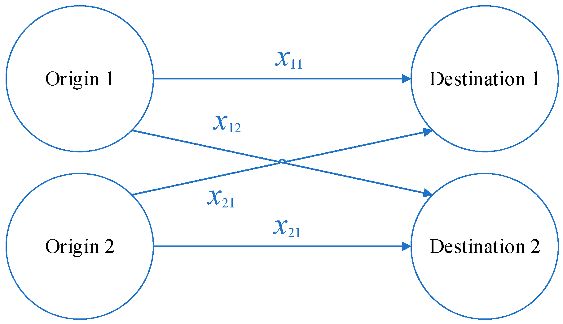
A system tends to evolve toward a particular steady state, and this steady state is called an attractor. The strange attractor in the attractor is of great significance for the study of chaotic systems [30,31,32,33,34]. Here, a gravity model with two origins and two destinations is used as an example to observe the dynamic behavior of the traffic network (Figure 1). With the initial conditions:

$$x(0)=\left[\begin{array}{cc}{x}_{11}(0)& x_{12}(0)\\ x_{21}(0)& x_{22}(0)\end{array}\right]=\left[\begin{array}{cc}0.03& 0.3521\\ 0.5313& 0.0866\end{array}\right]$$

(2)

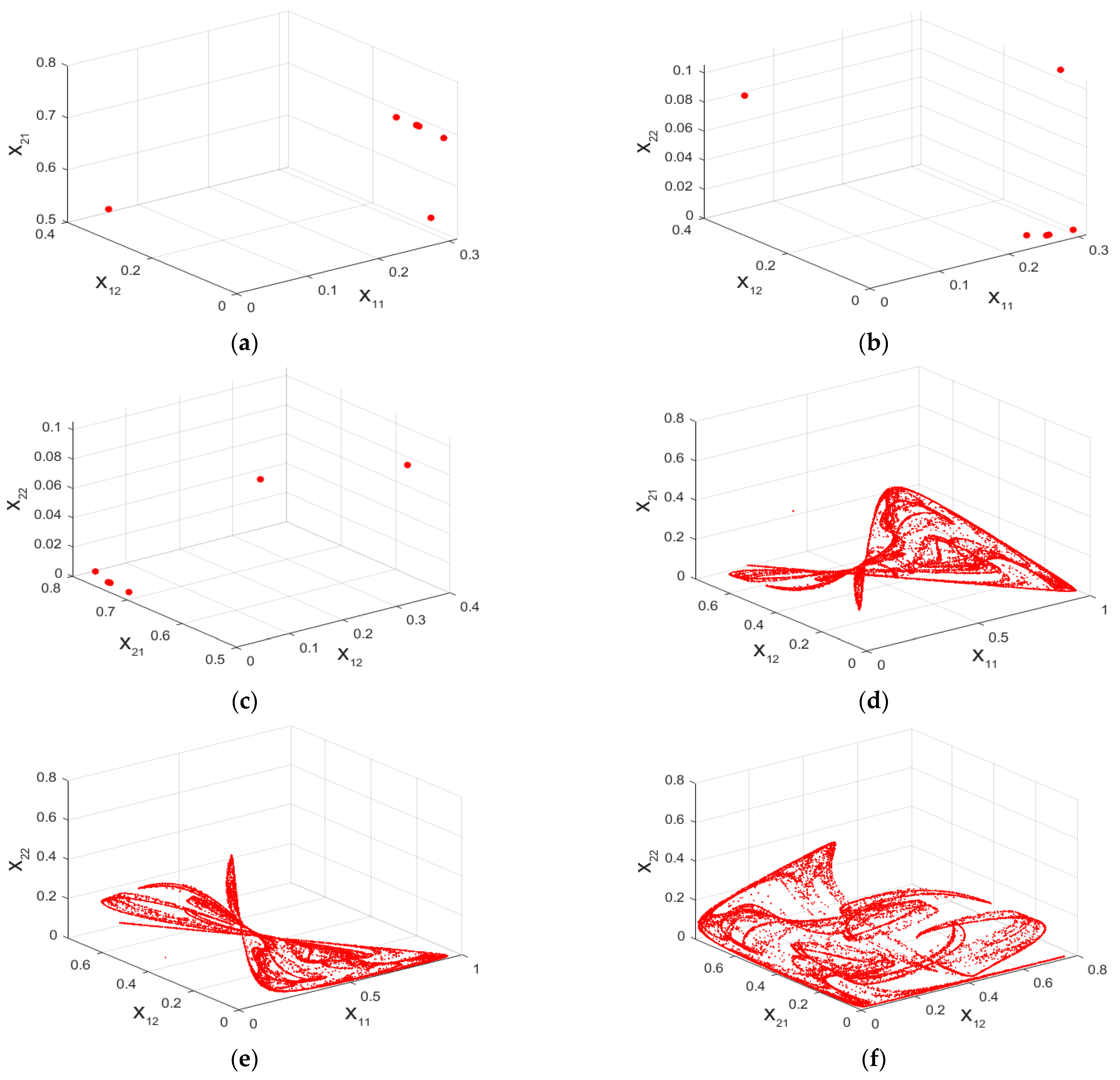
and the parameters $\alpha =1$, $\beta =3.25$, $\mu =6.5$, one can iterate model 1 until obtaining some attractors. As can be seen in Figure 2a–c, the traffic system is in a periodic state ($\gamma =1.69$). Figure 2d–f also indicate a phase trajectory with no evident periodic features and complicated structures of drawing back and folding ($\gamma =1$). As can be seen, they are in a limited area, and their movement is not what is expected because of the evident exponential divergence. The strange attractor has obvious fractal characteristics; its correlation dimension is 1.34412, and it has a butterfly phase trajectory similar to Lorenz system. The characteristics of this strange attractor reflect the self-organizing nature of traffic flow. The traffic flow system is neither deterministic nor completely stochastic. The change from orderly (smooth) to chaotic is due to the disturbance of various uncertainties within the system, which disrupts the original stable state. The shift from disorderly to orderly is due to the self-organization of traffic flow and the effect of proper management and control.

In Figure 1, $x_{ij}$ closely relates to realistic traffic factors such as speed, density, and headway time distance. The behavior of traffic flow subject traveling is a rational driving behavior. Safe, smooth, fast, and comfortable driving is the goal pursued by each individual. To achieve the common goal, participants cooperate and collaborate with each other so that the possibility of forming an orderly structure of traffic flow exists. The strange attractor in Figure 2 is the result of switching back and forth between this order and disorder, which has the fractal character of self-similarity.

3. An Improved Conical Volume-Delay Function

When travel units choose their travel routes by maximizing their interests, it may result in many travel units gathering on certain road sections at a specific moment. The difficulty that causes this phenomenon is that travel units do not fully understand the traffic conditions of the road network, choose the shortest route by estimating the time, and have preferences in choosing the route. At the same time, some road sections that seem to be very time-consuming but through which few travel units pass are almost idle. Therefore, we propose an improved conical volume-delay function as a new cost function [29]:

$$c^{*}(s_{ij})=c_{ij}^{(0)}(2+\sqrt{({\gamma }^2{(1-{\alpha }^{\frac{1}{\gamma }}{s}_{ij})}^2+{\theta }^2})-\gamma (1-{\alpha }^{\frac{1}{\gamma }}{s}_{ij})-\theta ),$$

(3)

where $\theta =\frac{2\gamma -1}{2\gamma -2}$, $\alpha >0$, $\gamma >1$.

Function (3) has the following properties:

(1) $c^{*}$ is a strictly increasing function.

(2) $c^{*}(0)=c_{ij}^{(0)}$, to ensure that the travel cost is free for roads with no flow.

(3) $c^{*}({\alpha }^{-\frac{1}{\gamma }})=2c_{ij}^{(0)}$. The special point ${\alpha }^{-\frac{1}{\gamma }}$ is considered here because $c({\alpha }^{-\frac{1}{\gamma }})=2c_{ij}^{(0)}$ in the original cost function. This means that in cases where the ratio of $x_{ij}$ to $q_{ij}$ is ${\alpha }^{-\frac{1}{\gamma }}$, the travel cost on the road equals twice the free travel cost. Hence, to ensure compatibility with the original cost function, this special point is considered in particular.

(4) $\frac{d^2(c^{*}(s_{ij}))}{d{s}_{ij}^2}>0$. This is similar the original cost function to ensure that $c^{*}$ is a convex function of $s_{ij}$.

(5) $\frac{d(c^{*}(s_{ij}))}{d{s}_{ij}}<M\gamma$, where $M$ is a finite normal number. This condition constrains the slope of the new cost function to ensure that change of $s_{ij}$ does not significantly affect the variation of the travel cost.

(6) ${\frac{d(c^{*}(s_{ij}))}{d{s}_{ij}}|}_{s_{ij}=0}>0$. This further ensures that the new cost function has a certain slope for a small value of $s_{ij}$.

The new cost function, $c^{*}(s_{ij})$, has properties (1)–(4) hence maintaining compatibility with the original cost function (1). To address the inherent all-or-nothing problem of the original cost function, properties (5) and (6) are added to the improved function. Substituting (1) with (3) in model 1, we then obtain the new model, namely model 2.

4. Dynamical Behavior of the New Model

The Lyapunov exponent is used to investigate how much attraction or separation exists between the two neighboring trajectories starting in different initial circumstances. It is an essential measure of the nonlinear system’s dynamic behavior defined based on its statistical properties [35]. For model $x_{n+1}=g(x_n)$, it has Lyapunov exponent

$$\lambda =\underset{n\to \infty }{\lim }\frac{1}{n}{\displaystyle \sum _{i=0}^{n-1}\ln \left|g^{\prime }(x_i)\right|}.$$

The motion states corresponding to different Lyapunov exponents are shown in

Table 1. The motion states corresponding to different Lyapunov exponents.

Lyapunov Exponent	Motion State
$\lambda <0$	periodic
$\lambda =0$	bifurcation
$\lambda >0$ (bounded system)	chaotic

.

Small disturbances, such as a vehicle’s acceleration or deceleration, might be passed to or exacerbated in the complex traffic. However, it appears that this is susceptible to the initial circumstances that generate chaos. Therefore, constructing a dynamic function that takes into account complicated aspects of the traffic flow system is generally challenging. To address this issue, we use the bifurcation diagram and time series analysis.

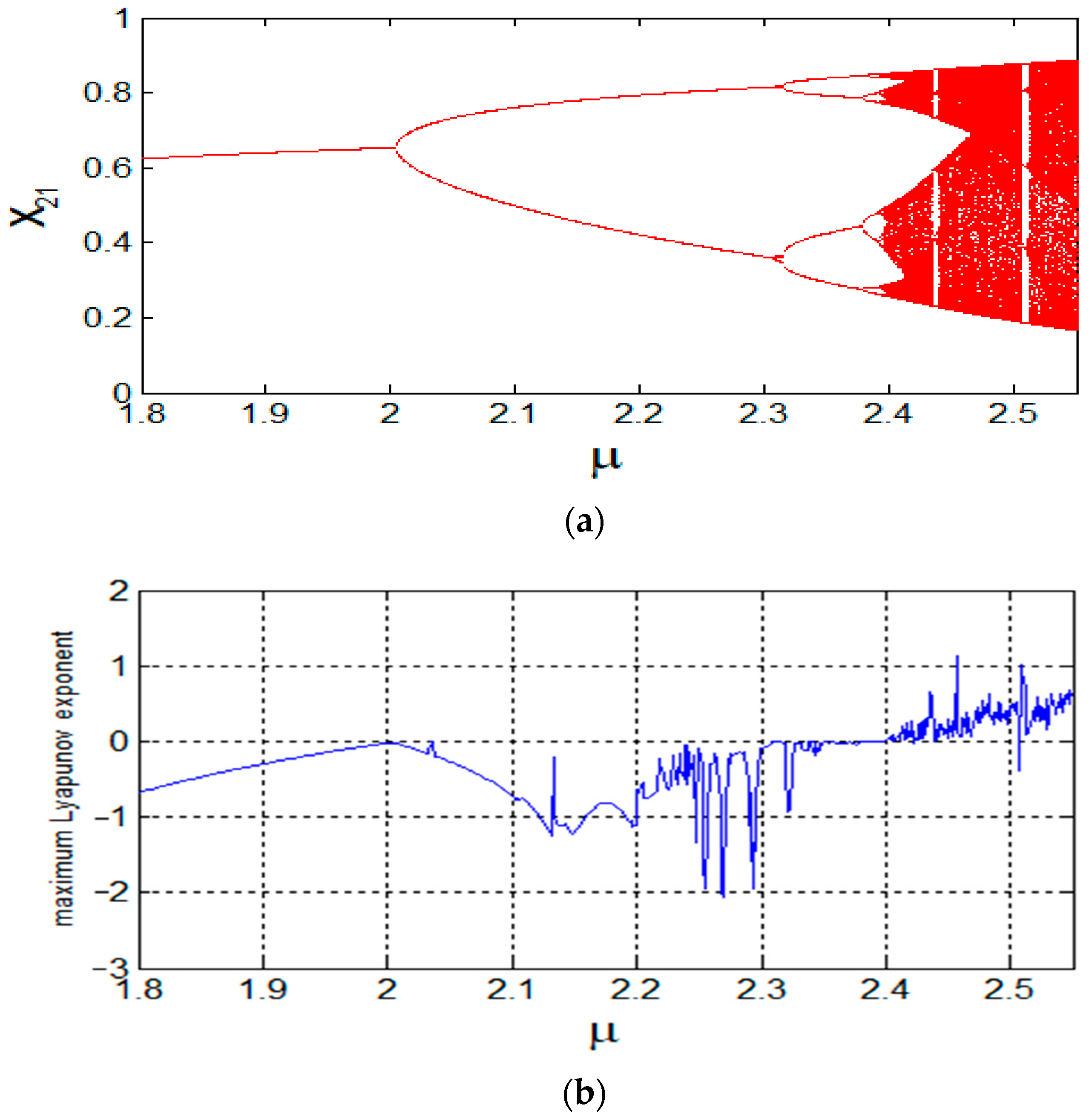
Here, in model 2, we set $\alpha =0.15$, $\beta =0.4$, $\gamma =2$, and the initial condition is also set to (2). Near $\mu =2$ (Figure 3a), there exists bifurcation and the model state changes from period-1 to period-2. By increasing $\mu$, the bifurcation happens again near $\mu =2.31$, and the model state changes from period-2 to period-4. Following several bifurcations, the model enters chaos again in the neighborhood of $\mu =2.39$. 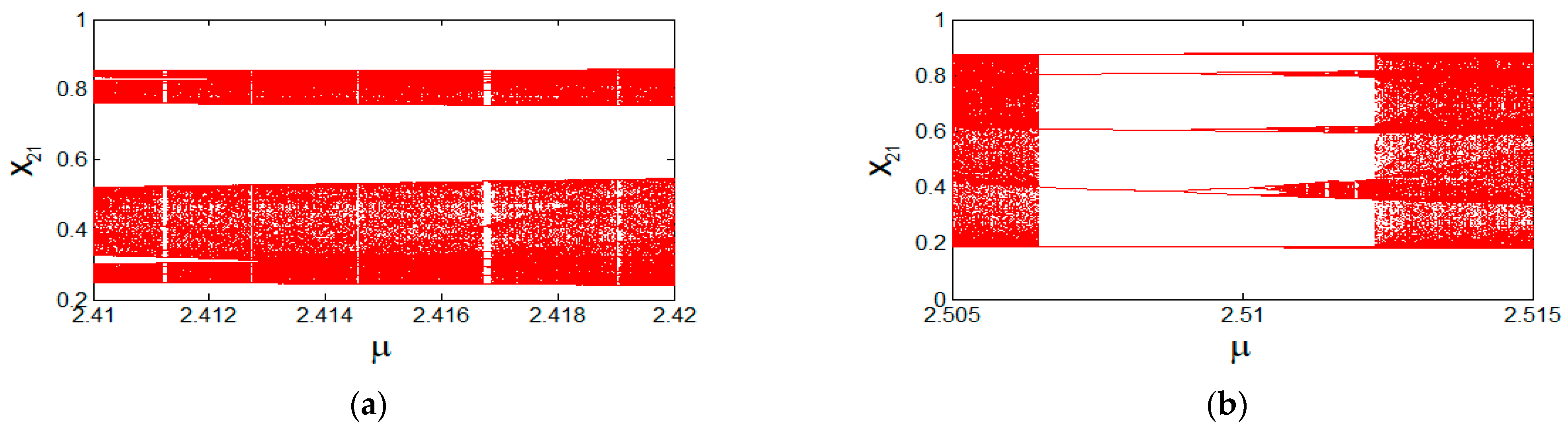In Figure 3a, the region $[2.41,2.42]$ is enlarged and shown in Figure 4a. Here, it is seen that the region alternates between chaos and periodic windows but is dominated by chaos. Figure 4b also shows the partial bifurcation sequences of Figure 3a in more detail. It is seen that period-doubling bifurcation to chaos occurs in the region $[2.505,2.515]$. Furthermore, it is also discovered that there are a few periodic windows in this chaotic region. As a result, the large periodic window contains many smaller periodic windows that behave in the same way as the period-doubling bifurcation behavior shown before. This local and global self-similar geometric structure reflects the fractal characteristics of model 2. For $\mu =2.54$, the model seems disordered (Figure 3a and Figure 5h), and the maximum Lyapunov exponent is 0.4584, hence the model is descended into chaos.

For cases where $\mu =2.39$, the traffic system is in a periodicity condition, and the travel units move steadily. It is seen that although the traffic system varies (e.g., due to external interference), re-entering the periodic motion can easily happen. This becomes the opposite for cases where $\mu$ is larger than 2.39. Although the traffic system runs smoothly within the chaotic region’s periodic window, once disturbed, it may be very easy to enter the chaos. This results in highly unpredictable traffic system operations. Hence, it is necessary to thoroughly study the characteristics of the system.

5. Three-Parameter Bifurcation

A three-parameter bifurcation diagram is a powerful tool for analyzing the traffic system’s dynamic behavior and making better parameter choices. Assuming the initial condition to be (2), and parameter $\alpha =0.15$, the three-parameter bifurcation diagrams of models 1 and 2 are drawn in the range of $\mu \in$ [2,5], $\beta \in [0.1,0.5]$, $\gamma \in [2,3]$ (Figure 6). Different colors are used to represent different periodic states of the system, and the color bar is marked with numbers on the right side of the figure. For instance, value 1 represents period-1, value 2 represents period-2,…, and value 199 represents period-199 (value 200 indicates that the period is greater than or equal to 200).

For a small value of parameter $\gamma$, the surface of the cube in Figure 6a indicates an obvious low periodicity, and the motion characteristics are relatively stable. By increasing $\gamma$, the low periodicity of the system gradually weakens and more regions with high periodicity appear. This indicates that the system is likely to frequently jump between order and chaos, confirming that model 1 is rather sensitive and might yield more complicated dynamic behavior.

The border between the blue and yellow areas is visible in Figure 6b. By changing the parameter values within a certain range, we also noticed that the colored areas are always relatively concentrated in the complete blue (low period) or yellow (high period) areas. This indicates that model 2 outperforms model 1 in terms of robustness and structural stability. This makes the traffic system unpredictable which might have an adverse effect on road traffic.

Figure 6c,d present the characteristics of the traffic system in more detail where the attributes of the color bars were changed and marked with corresponding numbers in the color bars on the right of the figure (value 20 indicates that the period is greater than or equal to 20). In Figure 6c, there is a clear boundary ($\gamma <2.4$) between the low and the high periodicity regions, and the low periodicity is mainly expressed in the form of period-1 to period-8. In Figure 6d, there is also a clear boundary between areas with low and high periodicities. The low periodicity of the lower area is mainly expressed in the form of period-1 to period-8, whereas the periodicity of the upper area is quite complex, including a variety of periodic forms.

To further understand the system, several screenshots of Figure 6a,b are shown in Figure 7. By comparing Figure 7a–c with Figure 7d–f, it is seen that model 2 shows a dominant low periodic state and is relatively stable. The high and low periodic states also frequently alternate in varying degrees. This makes the traffic system unpredictable, which might have an adverse effect on road traffic. In parameter optimization design, these particular values of parameters need to be avoided if possible.

6. All-or-Nothing Problem

When using the gravity model for traffic distribution, the traffic flows of the whole road network may converge on one path, resulting in some ways with no traffic flow. In practice, road designers try to avoid such cases before constructing the network so that the entire network is utilized as much as possible. Here, we introduce a metric value $T$ to quantify the extent to which the system addresses the all-or-nothing problem. The flowchart of obtaining $T$ is illustrated in Figure 8, where $\beta$, $\gamma$, and $\mu$ belong to $[{\beta }_1,{\beta }_{*}]$, $[{\gamma }_1,{\gamma }_{*}]$, and $[{\mu }_1,{\mu }_{*}]$, respectively, with the step sizes $h^{(\beta )}$, $h^{(\gamma )}$, and $h^{(\mu )}$. The sampling interval for the model O-D volume $x_{21}$ is $[a,b]$. The larger the value of $T$, the higher the risk of the all-or-nothing problem.

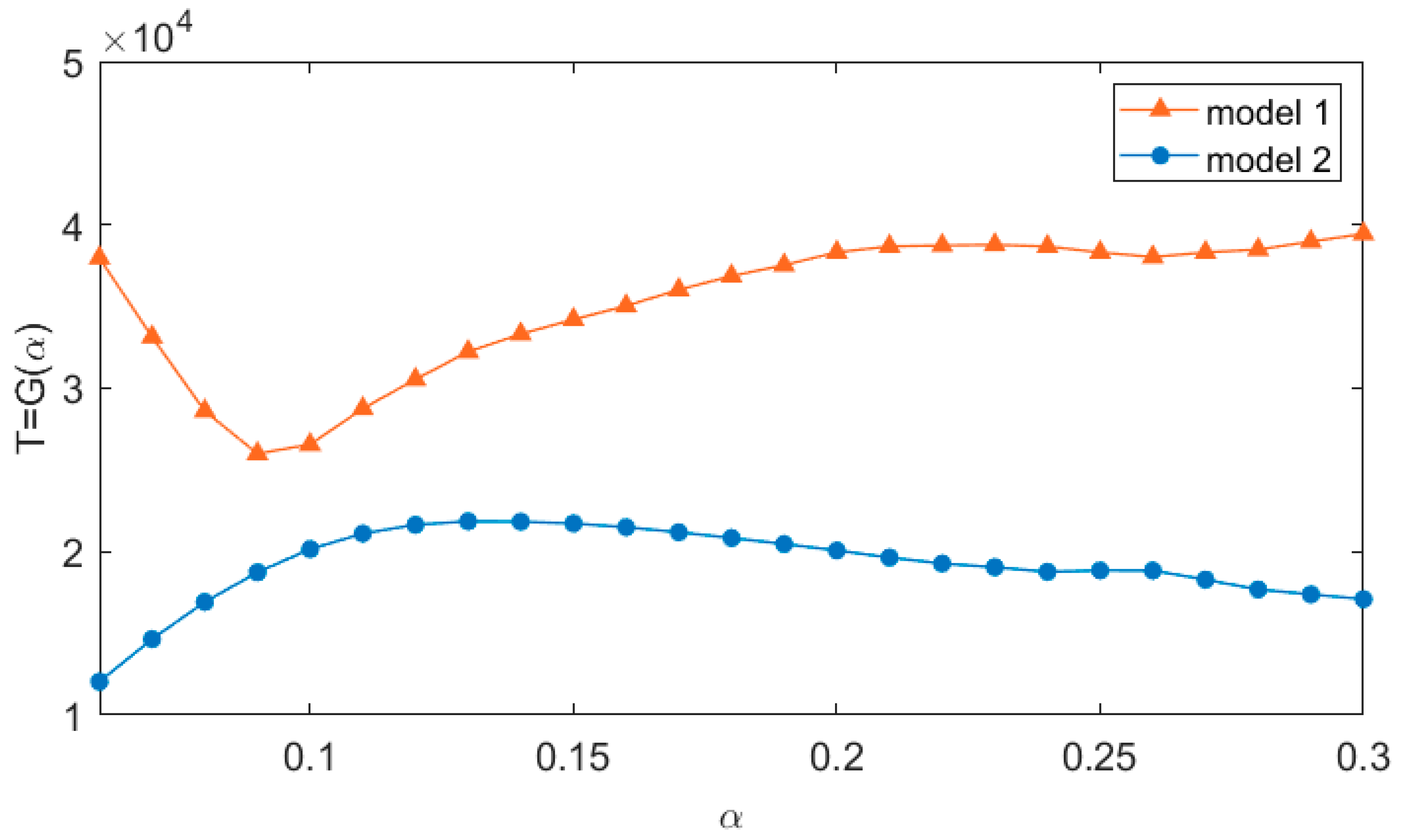
Adjusting the parameter $\alpha$ for the given model structure and initialization parameters results in changing $T$, where $T=G(\alpha )$. At this point, $\alpha$ and $T$ form a functional relationship, where $\alpha$ is the independent variable and $T$ is the dependent variable. The parameter $\alpha$ is taken between 0.06 and 0.3 with a step size of 0.01, and the rest of the initialization parameters are shown in

Table 2. The initial values of the model parameters.

Parameters	Value
$T$	$0$
$[{\beta }_1,{\beta }_{*}]$	$[0.1,0.5]$
$[{\gamma }_1,{\gamma }_{*}]$	$[2,3]$
$[{\mu }_1,{\mu }_{*}]$	$[2,5]$
$[a,b]$	$[401,500]$
$h^{(\beta )}$	$0.01$
$h^{(\gamma )}$	$0.02$
$h^{(\mu )}$	$0.05$

. Using these values, $T$ is plotted in Figure 9.

As can be seen in Figure 9, for a small $\alpha$, the metric function of model 1 follows a decreasing trend, where $T$ is at its lowest value for $\alpha =0.09$, followed by a gradual increase. For a small $\alpha$, the metric function of model 2 indicates a gradually increasing trend, where $T$ reaches its maximum value for $\alpha =0.13$, followed by a gradual decrease. Function $G$ for model 2 in Figure 9 is below the function $G$ of model 1.

The properties of (3) essentially determines this result. Property (5) constrains the slope of the new cost function (3) to ensure that the change of $x_{ij}$ does not significantly affect the variation of the travel cost. Property (6) ensures that (3) has a certain slope for a small value of $x_{ij}$. Hence, model 2 is significantly more effective than model 1 in dealing with the all-or-nothing traffic flow problem.

7. Conclusions

In this paper, we addressed the issues raised due to the deficiency of the original cost function by utilizing an improved conical volume-delay function. The improved conical volume-delay function has the main properties of the original cost function, and all its parameters have the same meaning as those in the original cost function. On this basis, the following conclusions were drawn based on analyzing the dynamical behavior of the traffic network and the model solutions: (1) the double-constrained dynamic gravity model with an improved conical volume-delay function has similar dynamic behavior to the previous model and can be adopted in investigating the O-D flow distribution; (2) three-parameter bifurcation confirms that the structural stability of the new model is higher than that of the previous model. The study also shows that when the new model is used, the traffic system is more likely to recover its steady state under external disturbances. Finally, (3) we further introduced a metric to assess the models’ capability to manage the all-or-nothing problem. Using this metric, we showed that the new dynamic gravity model handles this issue much more efficiently than the previous model.

This paper’s model parameters $\alpha$, $\beta$, $\gamma$, and $\mu$ are closely related to various aspects of the road network structure. Although they have no apparent physical significance, they can be calibrated based on traffic flow data. In the gravity model study, we use volume as the only input to the system, but the existing traffic system includes not only flow factors. Combining the gravity model with density, speed, and intersection factors can reveal the fractal characteristics of urban road traffic flow’s global and local relationships in more depth and provide an essential basis for intelligent transportation development.

References

- Fritzkowski, P.; Awrejcewicz, J. Near-resonant dynamics, period doubling and chaos of a 3-DOF vibro-impact system. Nonlinear Dyn. 2021, 106, 81–103. [Google Scholar] [CrossRef]
- Kamrani, A.; Zenkouar, K.; Najah, S. A new set of image encryption algorithms based on discrete orthogonal moments and Chaos theory. Multimed. Tools Appl. 2020, 79, 20263–20279. [Google Scholar] [CrossRef]
- Tian, Z. Preliminary research of chaotic characteristics and prediction of short-term wind speed time series. Int. J. Bifurc. Chaos 2020, 30, 2050176. [Google Scholar] [CrossRef]
- Sun, W.; Wang, Y.; Liu, F.; Wu, X. Applying explicit symplectic integrator to study chaos of charged particles around magnetized Kerr black hole. Eur. Phys. J. C 2021, 81, 785. [Google Scholar] [CrossRef]
- Naderi, B.; Kheiri, H. Exponential synchronization of chaotic system and application in secure communication. Optik 2016, 127, 2407–2412. [Google Scholar] [CrossRef]
- Cao, B.; Gu, H.; Bai, J.; Wu, F. Bifurcation and chaos of spontaneous oscillations of hair bundles in auditory hair cells. Int. J. Bifurc. Chaos 2021, 31, 2130011. [Google Scholar] [CrossRef]
- Turner, L. Driven-dissipative Euler’s equations for a rigid body: A chaotic system relevant to fluid dynamics. Phys. Rev. E 1996, 54, 5822–5825. [Google Scholar] [CrossRef]
- Feng, G. Chaotic dynamics and chaos control of Hassell-type recruitment population model. Discret. Dyn. Nat. Soc. 2020, 2020, 814863. [Google Scholar] [CrossRef] [Green Version]
- Doan, P.T.; Bui, P.D.H.; Vu, M.T.; Thanh, H.L.N.N.; Hossain, S. Stability analysis of a fractional-order high-speed supercavitating vehicle model with delay. Machines 2021, 9, 129. [Google Scholar] [CrossRef]
- Radu, V.; Dumitrescu, C.; Vasile, E.; Tanase, L.C.; Stefan, M.C.; Radu, F. Analysis of the Romanian Capital Market Using the Fractal Dimension. Fractal Fract. 2022, 6, 564. [Google Scholar] [CrossRef]
- Zhang, Y.; Luo, G. Detecting unstable periodic orbits and unstable quasiperiodic orbits in vibro-impact systems. Int. J. Non-Linear Mech. 2017, 96, 12–21. [Google Scholar] [CrossRef]
- Dubey, V.P.; Kumar, D.; Alshehri, H.M.; Dubey, S.; Singh, J. Computational analysis of local fractional LWR model occurring in a fractal vehicular traffic flow. Fractal Fract. 2022, 6, 426. [Google Scholar] [CrossRef]
- Wang, Z.; Chen, Y. Exploring spatial patterns of interurban passenger flows using dual gravity models. Entropy 2022, 24, 1792. [Google Scholar] [CrossRef]
- Lan, L.W.; Sheu, J.B.; Huang, Y.S. Investigation of temporal freeway traffic patterns in reconstructed state spaces. Transp. Res. Part C Emerg. Technol. 2008, 16, 116–136. [Google Scholar] [CrossRef]
- Guo, Y.M.; Yang, Z.; Zhou, Y.M.; Xiao, Z.B.; Yang, X.J. On the local fractional LWR model in fractal traffic flows in the entropy condition. Math. Methods Appl. Sci. 2017, 40, 55–61. [Google Scholar] [CrossRef]
- Halsey, T.C.; Jensen, M.H.; Kadanoff, L.P.; Procaccia, I.; Shraiman, B.I. Fractal measures and their singularities: The characterization of strange sets. Phys. Rev. A 1986, 33, 32–45. [Google Scholar] [CrossRef] [PubMed]
- Barrachina, X.; Conejero, J.A.; Murillo-Arcila, M.; Seoane-Sep’ulveda, J.B. Distributional chaos for the forward and backward control traffic model. Linear Algebra Its Appl. 2015, 479, 202–215. [Google Scholar] [CrossRef]
- Wu, X.; He, R.; He, M. Chaos analysis of urban low-carbon traffic based on game theory. Int. J. Environ. Res. Public Health 2021, 18, 2285. [Google Scholar] [CrossRef] [PubMed]
- Xue, J.N.; Shi, Z.K. Short-time traffic flow prediction based on chaos time series theory. J. Transp. Syst. Eng. Inf. Technol. 2008, 8, 68–72. [Google Scholar] [CrossRef]
- Gu, J.; Chen, S.Y.; Sivasundaram, S. Nonlinear analysis on traffic flow based on catastrophe and chaos theory. Discret. Dyn. Nat. Soc. 2014, 2014, 535167. [Google Scholar] [CrossRef] [Green Version]
- Wu, W.; Huang, N.; Wu, Z. Traffic chaotic dynamics modeling and analysis of deterministic network. Mod. Phys. Lett. B 2016, 30, 1650285. [Google Scholar] [CrossRef]
- Ashish; Cao, J.; Chugh, R. Chaotic behavior of logistic map in superior orbit and an improved chaos-based traffic control model. Nonlinear Dyn. 2018, 94, 959–975. [Google Scholar] [CrossRef]
- Boyce, D. Forecasting travel on congested urban transportation networks: Review and prospects for network equilibrium models. Netw. Spat. Econ. 2007, 7, 99–128. [Google Scholar] [CrossRef]
- Qian, J.H.; Han, D.D. Gravity model for transportation network based on optimal expected traffic. LNICST 2009, 4, 514–524. [Google Scholar] [CrossRef]
- Wang, Z.Y.; Chen, H.T.; Ou, Y.M. Research on regional traffic and economic linkage based on accessibility and gravity model-taking Hengyang, China as an example. IOP Conf. Ser. Earth Environ. Sci. 2020, 510, 062005. [Google Scholar] [CrossRef]
- Jung, W.S.; Wang, F.; Stanley, H.E. Gravity model in the Korean highway. EPL 2008, 81, 48005. [Google Scholar] [CrossRef] [Green Version]
- Wu, Z.; Huang, M.; Zhao, A.; Lan, Z. Urban traffic planning and traffic flow prediction based on ulchis gravity model and Dijkstra algorithm. J. Phys. Conf. Ser. 2021, 1972, 012080. [Google Scholar] [CrossRef]
- Zhang, X.Y.; David, F.J. Chaos in a dynamic model of traffic flows in an origin-destination network. Chaos Interdiscip. J. Nonlinear Sci. 1998, 8, 503–513. [Google Scholar] [CrossRef]
- Zhou, B.; Zhi, L.; Li, B. Improved BPR impedance function and its application in EMME. J. Shanghai Marit. Univ. 2013, 34, 67–70. [Google Scholar] [CrossRef]
- Zhang, Y.; Luo, G. Multistability of a three-degree-of-freedom vibro-impact system. Commun. Nonlinear Sci. 2018, 57, 331–341. [Google Scholar] [CrossRef]
- Ma, M.; Yang, Y.; Qiu, Z.; Peng, Y.; Sun, Y.; Li, Z.; Wang, M. A locally active discrete memristor model and its application in a hyperchaotic map. Nonlinear Dyn. 2022, 107, 2935–2949. [Google Scholar] [CrossRef]
- Peng, Y.; He, S.; Sun, K. Chaos in the discrete memristor-based system with fractional-order difference. Results Phys. 2021, 24, 104106. [Google Scholar] [CrossRef]
- Wang, N.; Zhang, G.; Kuznetsov, N.; Bao, H. Hidden attractors and multistability in a modified Chua’s circuit. Commun. Nonlinear Sci. 2021, 92, 105494. [Google Scholar] [CrossRef]
- Shen, Y.; Zhang, Y. Mechanisms of strange nonchaotic attractors in a nonsmooth system with border-collision bifurcations. Nonlinear Dyn. 2019, 96, 1405–1428. [Google Scholar] [CrossRef]
- Wolf, A.; Swift, J.; Swinney, H.L.; Vastano, J. Determing Lyapunov exponents from a time series. Phys. D Nonlinear Phenom. 1985, 16, 285–317. [Google Scholar] [CrossRef] [Green Version]