Efficient Spectral Collocation Method for Tempered Fractional Differential Equations

Abstract

Transient anomalous diffusion may be modeled by a tempered fractional diffusion equation. In this paper, we present a spectral collocation method with tempered fractional Jacobi functions (TFJFs) as basis functions and obtain an efficient algorithm to solve tempered-type fractional differential equations. We set up the approximation error as $O\left(N^{\mu -\nu }\right)$ for projection and interpolation by the TFJFs, which shows “spectral accuracy” for a certain class of functions. We derive a recurrence relation to evaluate the collocation differentiation matrix for implementing the spectral collocation algorithm. We demonstrate the effectiveness of the new method for the nonlinear initial and boundary problems, i.e., the fractional Helmholtz equation, and the fractional Burgers equation.

1. Introduction

Anomalous diffusion transport is often observed in nature and well described with fractional calculus (FC). Two kinds of anomalous diffusions are super diffusion and sub diffusion, according to the superlinear or sublinear growth of the variance of the variable of interest. Anomalous diffusion models, as the limit of a continuous time random walk (CTRW) with a heavy-tailed power–law probability distribution function, lead to diverging moments which can be problematic from a physical point of view. Exponentially tempering the power–law distributions is a popular way to temper the power–law distribution, which has both mathematical and technique advantages [1,2,3]. The FC involves an exponentially tempered factor, referred to as tempered fractional calculus (TFC), which describes the transition between normal and anomalous diffusions (or the anomalous motion in finite time or bounded physical space). TFC models have been applied in many scientific and engineering fields, such as poro-elasticity [4], ground water hydrology [5], geophysical flows [6], etc.

The application of TFC models to realistic problems requires numerical schemes that are available to solve the tempered fractional differential (TFD) equations. The difficulty of numerically solving the TFD equations is partially caused by the tempered fractional operators involving weak singular and exponential kernels. However, there is a lot of work that contributes to it. Li and Deng [7] presented the weighted and shifted Grünwald difference for the tempered fractional diffusion equations. Wang and Li [4] presented a fast difference scheme for a tempered fractional Burgers equation in porous media. Deng and Zhang [8] provided the variational formulation and efficient implementation for solving both spacial and temporal tempered fractional problems. Chen and Deng [9] proposed a second-order accurate numerical method for space–time tempered fractional diffusion–wave equations. Ding and Li [10] proposed a high-order algorithm for time-Caputo-tempered partial differential equations with Riesz derivatives in two spatial dimensions. Guo et al. [11] presented efficient fractional linear multistep methods for tempered fractional calculus. Cao et al. [12] studied finite difference/finite element methods for tempered time fractional advection–dispersion equations with fast evaluation of the Caputo derivative. Local discontinuous Galerkin methods were studied by Sun et al. [13] for the time-tempered fractional diffusion equation and by Safari et al. [14] for a class of time–space tempered fractional diffusion equations. Bu and Oosterlee [15] proposed a multigrid method for tempered fractional diffusion equations. Çelik and Duman [16] studied the finite element method for a symmetric tempered fractional diffusion equation. Zayernouri et al. [17] studied two classes of regular and singular tempered fractional Sturm–Liouville problems, in which a Petrov–Galerkin spectral method for solving tempered fractional ODEs is developed, and the tempered Jacobi poly-fractonomials are used as basis functions. Hanert and Piret [18] proposed a Chebyshev pseudospectral method to solve the space–time tempered fractional diffusion equation. Chen et al. [19] considered a Laguerre spectral-Galerkin method for solving tempered fractional diffusion equations on unbounded domain. Luo et al. [20] presented a Lagrange-quadratic spline optimal collocation method for the time-tempered fractional diffusion equation. Moghaddam et al. [21] suggested sinc collocation for the TFD equation, and Liemert and Kienle [22] used the Fourier spectral method to solve the tempered fractional wave–diffusion equation.

Meanwhile, Li et al. [23] discussed the existence, uniqueness, and stability of the tempered fractional ordinary differential equations. Deng et al. [24] discussed the reflecting boundaries for tempered fractional diffusion operators in the context of demonstrating the well-posedness of PDEs with generalized boundary conditions. From a mathematical view, the tempered fractional calculus operators are equivalent to the fractional substantial calculus after a suitable range of parameters [25]. One can also refer to [26,27] and references therein for the numerical methods of the substantial fractional differential equations.

Motivated by the generalized Jacobi functions in [28] and the method in [17], we aim to develop a high-accuracy spectral collocation method that uses the tempered fractional Jacobi functions (TFJFs) as the basis functions for solving TFD equations in this work. The main contributions of this paper are as follows:

†

We define the TFJFs and derive the approximation results of orthogonal projection and interpolation based on the TFJFs.

†

We derive the differentiation matrix of the tempered fractional Caputo derivative and give a fast and stable evaluation method based on the recurrence relationship.

†

We demonstrate the effectiveness of the proposed spectral collocation method for the initial or boundary value problems, i.e., the fractional Helmholtz equation, and the fractional Burgers equation.

The outline of the paper is as follows. In the next section, we review some definitions and properties of tempered fractional calculus. We also define the TFJFs and show their properties. We present the approximation properties based on the TFJFs in Section 3. In Section 4, we present the spectral collocation method based on the TFJFs and derive a recurrence relation for the fast generation of the collocation fractional differentiation matrix. Finally, we discuss the condition number of the fractional differentiation matrix. In Section 5, we apply the spectral collocation to the initial value problems of nonlinear fractional ordinary differential equation. In Section 6, we apply the spectral collocation to the fractional Helmholtz equation and the fractional Burgers equation. Several numerical tests are presented in this section. The paper ends with some conclusions in Section 7.

2. Preliminaries

2.1. Definitions of Tempered Fractional Calculus

In the sequence, we start with the definitions of tempered fractional operators.

Definition 1.

For $\kappa \ge 0$, the left and right tempered fractional integrals of function $u\left(t\right)$ on $(a,b)$ of order $\mu >0$ are defined, respectively, by [5,8,29]

$${{}_a\mathrm{I}}_t^{\mu ,\kappa }u\left(t\right):=\frac{1}{\Gamma \left(\mu \right)}{\int }_a^t\frac{e^{-\kappa (t-s)}u\left(s\right)}{{(t-s)}^{1-\mu }}\mathrm{d}s,{{}_t\mathrm{I}}_b^{\mu ,\kappa }u\left(t\right):=\frac{1}{\Gamma \left(\mu \right)}{\int }_t^b\frac{e^{-\kappa (s-t)}u\left(s\right)}{{(s-t)}^{1-\mu }}\mathrm{d}s,$$

where $\Gamma (·)$ is the Euler gamma function.

Definition 2.

For $\kappa \ge 0$, the left and right tempered Riemman–Liouville fractional derivatives of function $u\left(t\right)$ on $(a,b)$ of order $\mu >0$ are defined, respectively, by [5,8,29]

$${{}_a^R\mathrm{D}}_t^{\mu ,\kappa }u\left(t\right):=\frac{e^{-\kappa t}}{\Gamma (n-\mu )}\frac{{\mathrm{d}}^n}{\mathrm{d}{t}^n}{\int }_a^t\frac{e^{\kappa s}u\left(s\right)}{{(t-s)}^{\mu -n+1}}\mathrm{d}s,$$

and

$${{}_t^R\mathrm{D}}_b^{\mu ,\kappa }u\left(t\right):=\frac{e^{\kappa t}}{\Gamma (n-\mu )}\frac{{\mathrm{d}}^n}{\mathrm{d}{t}^n}{\int }_t^b\frac{e^{-\kappa s}u\left(s\right)}{{(s-t)}^{\mu -n+1}}\mathrm{d}s,$$

where $n-1<\mu \le n.$

By direct calculation, the following relations are obtained:

$${{}_a^R\mathrm{D}}_t^{\mu ,\kappa }u\left(t\right):={\left(\frac{\mathrm{d}}{\mathrm{d}t}+\kappa \right)}^n{{}_a\mathrm{I}}_t^{n-\mu ,\kappa }u\left(t\right),$$

and

$${{}_t^R\mathrm{D}}_b^{\mu ,\kappa }u\left(t\right):={(-1)}^n{\left(\frac{\mathrm{d}}{\mathrm{d}t}-\kappa \right)}^n{{}_t\mathrm{I}}_b^{n-\mu ,\kappa }u\left(t\right),$$

where ${\left(\frac{\mathrm{d}}{\mathrm{d}t}\pm \kappa \right)}^n={\sum }_{k=0}^n\frac{k!(n-k)!}{n!}{(\pm \kappa )}^{n-k}\frac{{\mathrm{d}}^k}{\mathrm{d}{t}^k}.$

Definition 3.

For $\kappa \ge 0$, the left and right tempered Caputo fractional derivatives of function $u\left(t\right)$ on $(a,b)$ of order $\mu >0$ are defined by [8,23]

$${{}_a^C\mathrm{D}}_t^{\mu ,\kappa }u\left(t\right):={{}_a\mathrm{I}}_t^{n-\mu ,\kappa }{\left(\frac{\mathrm{d}}{\mathrm{d}t}+\kappa \right)}^{n}u\left(t\right)=\frac{e^{-\kappa t}}{\Gamma (n-\mu )}{\int }_a^t\frac{{\left(e^{\kappa s}u\left(s\right)\right)}^{\left(n\right)}}{{(t-s)}^{\mu -n+1}}\mathrm{d}s,$$

and

$${{}_t^C\mathrm{D}}_b^{\mu ,\kappa }u\left(t\right):={{}_t\mathrm{I}}_b^{n-\mu ,\kappa }{(-1)}^n{\left(\frac{\mathrm{d}}{\mathrm{d}t}-\kappa \right)}^{n}u\left(t\right)=\frac{{(-1)}^n{e}^{\kappa t}}{\Gamma (n-\mu )}{\int }_t^b\frac{{\left(e^{-\kappa s}u\left(s\right)\right)}^{\left(n\right)}}{{(s-t)}^{\mu -n+1}}\mathrm{d}s,$$

where $n-1<\mu \le n.$

If $\kappa \equiv 0$, then the left and right tempered fractional calculus reduce to the left and right (non-tempered) fractional calculus, denoted by ${}_a{\mathrm{I}}_t^{\mu },{}_t{\mathrm{I}}_b^{\mu },{}_a^R{\mathrm{D}}_t^{\mu },{}_t^R{\mathrm{D}}_b^{\mu },{}_a^C{\mathrm{D}}_t^{\mu }$ and ${}_t^C{\mathrm{D}}_b^{\mu }$, respectively. Then, we have

$$\begin{array}{cc}\hfill {{}_a\mathrm{I}}_t^{\mu ,\kappa }u\left(t\right)& =e^{-\kappa t}{}_a{\mathrm{I}}_t^{\mu }\left(e^{\kappa t}u\left(t\right)\right),{{}_t\mathrm{I}}_b^{\mu ,\kappa }u\left(t\right)=e^{\kappa t}{}_t{\mathrm{I}}_b^{\mu }\left(e^{-\kappa t}u\left(t\right)\right),\hfill \\ \hfill {{}_a^R\mathrm{D}}_t^{\mu ,\kappa }u\left(t\right)& =e^{-\kappa t}{}_a^R{\mathrm{D}}_t^{\mu }\left(e^{\kappa t}u\left(t\right)\right),{{}_t^R\mathrm{D}}_b^{\mu ,\kappa }u\left(t\right)=e^{\kappa t}{}_t^R{\mathrm{D}}_b^{\mu }\left(e^{-\kappa t}u\left(t\right)\right),\hfill \\ \hfill {{}_a^C\mathrm{D}}_t^{\mu ,\kappa }u\left(t\right)& =e^{-\kappa t}{}_a^C{\mathrm{D}}_t^{\mu }\left(e^{\kappa t}u\left(t\right)\right),{{}_t^C\mathrm{D}}_b^{\mu ,\kappa }u\left(t\right)=e^{\kappa t}{}_t^C{\mathrm{D}}_b^{\mu }\left(e^{-\kappa t}u\left(t\right)\right).\hfill \end{array}$$

Similar to the corresponding non-tempered case, for $0<\mu <1$ and $u\left(t\right)$ be absolutely continuous in $[a,b]$, the relations between the Riemann–Liouville and Caputo derivatives are

$${}_a^R{\mathrm{D}}_t^{\mu ,\kappa }u\left(t\right)={}_a^C{\mathrm{D}}_t^{\mu ,\kappa }u\left(t\right)+\frac{1}{\Gamma (1-\mu )}{e}^{-\kappa t}{(t-a)}^{-\mu }u\left(a\right),$$

(1)

and

$${}_t^R{\mathrm{D}}_b^{\mu ,\kappa }u\left(t\right)={}_t^C{\mathrm{D}}_b^{\mu ,\kappa }u\left(t\right)+\frac{1}{\Gamma (1-\mu )}{e}^{-\kappa t}{(b-t)}^{-\mu }u\left(b\right).$$

(2)

For practical purposes, we consider the linear transform from $[a,b]$ to $[-1,1]$ as

$$s=\frac{2(t-a)}{b-a}-1,t\in [a,b](ort=\frac{b-a}{2}(s+1)+a,s\in [-1,1]).$$

Then, it holds that

$${{}_a\mathrm{I}}_t^{\mu ,\kappa }u\left(t\right)={\left(\frac{b-a}{2}\right)}^{\mu }{{}_{-1}\mathrm{I}}_s^{\mu ,\tilde{\kappa }}\tilde{u}\left(s\right),{{}_t\mathrm{I}}_b^{\mu ,\kappa }u\left(t\right)={\left(\frac{b-a}{2}\right)}^{\mu }{{}_s\mathrm{I}}_1^{\mu ,\tilde{\kappa }}\tilde{u}\left(s\right),$$

and

$${{}_a^C\mathrm{D}}_t^{\mu ,\kappa }u\left(t\right)={\left(\frac{2}{b-a}\right)}^{\mu }{{}_{-1}^C\mathrm{D}}_s^{\mu ,\tilde{\kappa }}\tilde{u}\left(s\right),{{}_t^C\mathrm{D}}_b^{\mu ,\kappa }u\left(t\right)={\left(\frac{2}{b-a}\right)}^{\mu }{{}_s^C\mathrm{D}}_1^{\mu ,\tilde{\kappa }}\tilde{u}\left(s\right),$$

where $\tilde{\kappa }=\frac{b-a}{2}\kappa ,\tilde{u}\left(s\right)=u\left(t\right)=u(\frac{b-a}{2}(s+1)+a).$

2.2. Tempered Fractional Jacobi Functions (TFJFs)

In this subsection, we introduce the TFJFs and derive some properties for use. Denote ${\mathbb{P}}_N\left(I\right)$ as the space of all algebraic polynomials with degree at most N defined on $I=:(-1,1)$. Let $P_n^{\alpha ,\beta }\left(s\right)(\alpha ,\beta >-1),s\in I$ be the Jacobi orthogonal polynomials, satisfying

$${\int }_{-1}^1{P}_n^{\alpha ,\beta }\left(s\right)P_m^{\alpha ,\beta }\left(s\right){\omega }^{\alpha ,\beta }\left(s\right)\mathrm{d}s={\gamma }_n^{\alpha ,\beta }{\delta }_{mn},$$

(3)

where ${\omega }^{\alpha ,\beta }\left(s\right)={(1-s)}^{\alpha }{(1+s)}^{\beta }$,

$${\gamma }_n^{\alpha ,\beta }=\frac{2^{\alpha +\beta +1}\Gamma (n+\alpha +1)\Gamma (n+\beta +1)}{(2n+\alpha +\beta +1)n!\Gamma (n+\alpha +\beta +1)},$$

and ${\delta }_{mn}$ is the Kronecker symbol, i.e.,

$${\delta }_{mn}=\left\{\begin{array}{cc}1,\hfill & \mathrm{if}m=n,\hfill \\ 0,\hfill & \mathrm{otherwise}.\hfill \end{array}\right.$$

The derivative relation of the Jacobi polynomials is of importance:

$$\frac{{\mathrm{d}}^k}{\mathrm{d}{s}^k}{P}_n^{\alpha ,\beta }\left(s\right)=d_{n,k}^{\alpha ,\beta }{P}_{n-k}^{\alpha +k,\beta +k}\left(s\right),d_{n,k}^{\alpha ,\beta }=\frac{\Gamma (n+k+\alpha +\beta +1)}{2^k\Gamma (n+\alpha +\beta +1)},n\ge k.$$

(4)

The following relation is useful:

$$P_n^{\alpha ,\beta }\left(s\right)=\frac{\mathrm{d}}{\mathrm{d}s}\left[{\widehat{A}}_n^{\alpha ,\beta }{P}_{n-1}^{\alpha ,\beta }\left(s\right)+{\widehat{B}}_n^{\alpha ,\beta }{P}_n^{\alpha ,\beta }\left(s\right)+{\widehat{C}}_n^{\alpha ,\beta }{P}_{n+1}^{\alpha ,\beta }\left(s\right)\right],$$

(5)

where

$$\left\{\begin{array}{cc}\hfill {\widehat{A}}_n^{\alpha ,\beta }& =\frac{-2(n+\alpha )(n+\beta )}{(n+\alpha +\beta )(2n+\alpha +\beta )(2n+\alpha +\beta +1)},\hfill \\ \hfill {\widehat{B}}_n^{\alpha ,\beta }& =\frac{2(\alpha -\beta )}{(2n+\alpha +\beta )(2n+\alpha +\beta +2)},\hfill \\ \hfill {\widehat{C}}_n^{\alpha ,\beta }& =\frac{2(n+\alpha +\beta +1)}{(2n+\alpha +\beta +1)(2n+\alpha +\beta +2)}.\hfill \end{array}\right.$$

(6)

Some additional properties of Jacobi polynomials can be referred to [30,31].

Definition 4.

Define the TFJFs by

$$J_{n,l}^{\alpha ,\beta ,\delta ,\kappa }\left(s\right)=:e^{-\kappa s}{(1+s)}^{\delta }{P}_n^{\alpha ,\beta }\left(s\right),J_{n,r}^{\alpha ,\beta ,\delta ,\kappa }\left(s\right)=:e^{\kappa s}{(1-s)}^{\delta }{P}_n^{\alpha ,\beta }\left(s\right),$$

for $s\in I,n=0,1,\cdots .$

From the properties of Jacobi polynomials and Definition 4, we can easily derive the following lemma:

Lemma 1.

The TFJFs have the following properties.

P1. 

Three-term recurrence relation: For $n\ge 1$,

$$\left\{\begin{array}{c}{\displaystyle J_{n+1,l}^{\alpha ,\beta ,\delta ,\kappa }\left(s\right)=\left(A_n^{\alpha ,\beta }s-B_n^{\alpha ,\beta }\right)J_{n,l}^{\alpha ,\beta ,\delta ,\kappa }\left(s\right)-C_n^{\alpha ,\beta }{J}_{n-1,l}^{\alpha ,\beta ,\delta ,\kappa }\left(s\right),}\hfill \\ J_{n+1,r}^{\alpha ,\beta ,\delta ,\kappa }\left(s\right)=\left(A_n^{\alpha ,\beta }s-B_n^{\alpha ,\beta }\right)J_{n,r}^{\alpha ,\beta ,\delta ,\kappa }\left(s\right)-C_n^{\alpha ,\beta }{J}_{n-1,r}^{\alpha ,\beta ,\delta ,\kappa }\left(s\right),\hfill \end{array}\right.$$

(7)

with starting terms

$$\left\{\begin{array}{c}{\displaystyle J_{0,l}^{\alpha ,\beta ,\delta ,\kappa }\left(s\right)=e^{-\kappa s}{(1+s)}^{\delta },}\hfill \\ {\displaystyle J_{1,l}^{\alpha ,\beta ,\delta ,\kappa }\left(s\right)=e^{-\kappa s}{(1+s)}^{\delta }\left(\frac{\alpha +\beta +2}{2}s+\frac{\alpha -\beta }{2}\right),}\hfill \\ {\displaystyle J_{0,r}^{\alpha ,\beta ,\delta ,\kappa }\left(s\right)=e^{\kappa s}{(1-s)}^{\delta },}\hfill \\ {\displaystyle J_{1,r}^{\alpha ,\beta ,\delta ,\kappa }\left(s\right)=e^{\kappa s}{(1-s)}^{\delta }\left(\frac{\alpha +\beta +2}{2}s+\frac{\alpha -\beta }{2}\right),}\hfill \end{array}\right.$$

(8)

where

$$\left\{\begin{array}{cc}{A}_n^{\alpha ,\beta }\hfill & {\displaystyle =\frac{(2n+\alpha +\beta +1)(2n+\alpha +\beta +2)}{2(n+1)(n+\alpha +\beta +1)},}\hfill \\ B_n^{\alpha ,\beta }\hfill & {\displaystyle =\frac{(2n+\alpha +\beta +1)(2n+\alpha +\beta +2)}{2(n+1)(n+\alpha +\beta +1)},}\hfill \\ C_n^{\alpha ,\beta }\hfill & {\displaystyle =\frac{(n+\alpha )(n+\beta )(2n+\alpha +\beta +2)}{(n+1)(n+\alpha +\beta +1)(2n+\alpha +\beta )}.}\hfill \end{array}\right.$$

P2. 

Orthogonality: For $\alpha ,\beta >-1$,

$${\int }_I{J}_{n,l}^{\alpha ,\beta ,\delta ,\kappa }\left(s\right)J_{m,l}^{\alpha ,\beta ,\delta ,\kappa }\left(x\right){\varpi }_l^{\alpha ,\beta ,\delta ,\kappa }\left(s\right)\mathrm{d}s={\gamma }_n^{\alpha ,\beta }{\delta }_{nm},$$

(9)

$${\int }_I{J}_{n,r}^{\alpha ,\beta ,\delta ,\kappa }\left(s\right)J_{m,r}^{\alpha ,\beta ,\delta ,\kappa }\left(x\right){\varpi }_r^{\alpha ,\beta ,\delta ,\kappa }\left(s\right)\mathrm{d}s={\gamma }_n^{\alpha ,\beta }{\delta }_{nm},$$

(10)

$${\int }_I{J}_{n,l}^{\alpha ,\beta ,\delta ,\kappa }\left(s\right)J_{m,r}^{\alpha ,\beta ,\delta ,\kappa }\left(x\right){\varpi }_h^{\alpha ,\beta ,\delta }\left(s\right)\mathrm{d}s={\gamma }_n^{\alpha ,\beta }{\delta }_{nm},$$

(11)

where

$$\begin{array}{cc}\hfill {\varpi }_l^{\alpha ,\beta ,\delta ,\kappa }\left(s\right)& =e^{2\kappa s}{\omega }^{\alpha ,\beta -2\delta }\left(s\right)=e^{2\kappa s}{(1-s)}^{\alpha }{(1+s)}^{\beta -2\delta },\hfill \\ \hfill {\varpi }_r^{\alpha ,\beta ,\delta ,\kappa }\left(s\right)& =e^{-2\kappa s}{\omega }^{\alpha -2\delta ,\beta }\left(s\right)=e^{-2\kappa s}{(1-s)}^{\alpha -2\delta }{(1+s)}^{\beta },\hfill \\ \hfill {\varpi }_h^{\alpha ,\beta ,\delta ,\kappa }\left(s\right)& ={\omega }^{\alpha -\delta ,\beta -\delta }\left(s\right)={(1-s)}^{\alpha -\delta }{(1+s)}^{\beta -\delta }.\hfill \end{array}$$

Proof. 

The three-term recurrence relation given by Equation (7) is a straightforward result from the corresponding relation of Jacobi polynomials.

We derive, from Definition 4, that

$${\int }_I{J}_{n,l}^{\alpha ,\beta ,\delta ,\kappa }\left(s\right)J_{m,l}^{\alpha ,\beta ,\delta ,\kappa }\left(s\right){\varpi }_l^{\alpha ,\beta ,\delta ,\kappa }\left(s\right)\mathrm{d}s={\int }_I{P}_n^{\alpha ,\beta }\left(s\right)P_m^{\alpha ,\beta }\left(s\right){\omega }^{\alpha ,\beta }\left(s\right)\mathrm{d}s.$$

Then, we have the orthogonality (9). We can derive the other equalities (10) and (11) similarly. This ends the proof. □

Remark 1.

The orthogonalities (9) and (10) are in the inner product of space $L_{{\varpi }_l^{\alpha ,\beta ,\delta ,\kappa }}\left(I\right)$ and $L_{{\varpi }_r^{\alpha ,\beta ,\delta ,\kappa }}\left(I\right)$, respectively. The relationship (11) means that elements between the two above spaces are under measure ${\varpi }_h^{\alpha ,\beta ,\delta ,\kappa }$.

The tempered fractional derivatives of the TFJFs can also be represented by the same class of functions.

Theorem 1.

For $n\ge 0$, there holds

$$\begin{array}{cc}\hfill {{}_{-1}^R\mathrm{D}}_s^{\mu ,\kappa }\left(J_{n,l}^{\alpha ,\beta ,\beta ,\kappa }\left(s\right)\right)& ={\lambda }_n^{\beta ,\mu }{J}_{n,l}^{\alpha +\mu ,\beta -\mu ,\beta -\mu ,\kappa }\left(s\right),\alpha \in \mathbb{R},\beta >\mu -1.\hfill \\ \hfill {{}_s^R\mathrm{D}}_1^{\mu ,\kappa }\left(J_{n,r}^{\alpha ,\beta ,\alpha ,\kappa }\left(s\right)\right)& ={\lambda }_n^{\alpha ,\mu }{J}_{n,r}^{\alpha -\mu ,\beta +\mu ,\alpha -\mu ,\kappa }\left(s\right),\alpha >\mu -1,\beta \in \mathbb{R}.\hfill \end{array}$$

where

$${\lambda }_n^{\beta ,\mu }=\frac{\Gamma (n+\beta +1)}{\Gamma (n+\beta -\mu +1)}.$$

Proof. 

From Definitions 4, we have

$${{}_{-1}^R\mathrm{D}}_s^{\mu ,\kappa }\left(J_{n,l}^{\alpha ,\beta ,\beta ,\kappa }\left(s\right)\right)=e^{-\kappa s}{{}_{-1}^R\mathrm{D}}_s^{\mu }\left({(1+s)}^{\beta }{P}_n^{\alpha ,\beta }\left(s\right)\right).$$

Then, by Theorem 3.1 in [28], where

$${{}_{-1}^R\mathrm{D}}_s^{\mu }\left({(1+s)}^{\beta }{P}_n^{\alpha ,\beta }\left(s\right)\right)={\lambda }_n^{\beta ,\mu }{(1+s)}^{\beta -\mu }{P}_n^{\alpha +\mu ,\beta -\mu }\left(s\right),$$

the desired result can be obtained. The second equality is derived similarly. □

3. Approximation by the TFJFs

3.1. Error Estimate of Projection Operators

We introduce the $(N+1)$-dimensional spaces of the TFJFs as

$${\mathbb{F}}_{N,l}^{\delta ,\kappa }:=e^{-\kappa s}{(1+s)}^{\delta }{\mathbb{P}}_N=span\left\{J_{0,l}^{\alpha ,\beta ,\delta ,\kappa },J_{1,l}^{\alpha ,\beta ,\delta ,\kappa },\cdots ,J_{N,l}^{\alpha ,\beta ,\delta ,\kappa }\right\},$$

and

$${\mathbb{F}}_{N,r}^{\delta ,\kappa }:=e^{\kappa s}{(1-s)}^{\delta }{\mathbb{P}}_N=span\left\{J_{0,r}^{\alpha ,\beta ,\delta ,\kappa },J_{1,r}^{\alpha ,\beta ,\delta ,\kappa },\cdots ,J_{N,r}^{\alpha ,\beta ,\delta ,\kappa }\right\}.$$

Let $\alpha ,\beta >-1$. Denote ${\mathbf{P}}_{N,l}^{\delta ,\kappa }:L_{{\varpi }_l^{\alpha ,\beta ,\delta ,\kappa }}^2\left(I\right)\to {\mathbb{F}}_{N,l}^{\delta ,\kappa }$ as the orthogonal projection such that

$${({\mathbf{P}}_{N,l}^{\delta ,\kappa }u-u,v)}_{{\varpi }_l^{\alpha ,\beta ,\delta ,\kappa }}=0\forall v\in {\mathbb{F}}_{N,l}^{\delta ,\kappa },$$

(12)

and ${\mathbf{P}}_{N,r}^{\delta ,\kappa }:L_{{\varpi }_r^{\alpha ,\beta ,\delta ,\kappa }}^2\left(I\right)\to {\mathbb{F}}_{N,r}^{\delta ,\kappa }$ as the orthogonal projection such that

$${({\mathbf{P}}_{N,r}^{\delta ,\kappa }u-u,v)}_{{\varpi }_r^{\alpha ,\beta ,\delta ,\kappa }}=0\forall v\in {\mathbb{F}}_{N,r}^{\delta ,\kappa }.$$

(13)

Consider ${\mathbf{P}}_{N,l}^{\delta ,\kappa }$. One can express the orthogonal projection as

$${\mathbf{P}}_{N,l}^{\delta ,\kappa }u\left(s\right)=\sum _{k=0}^N{\widehat{u}}_k{J}_{k,l}^{\alpha ,\beta ,\delta ,\kappa }\left(s\right),$$

(14)

with

$${\widehat{u}}_k=\frac{{\int }_{-1}^{1}u\left(s\right)J_{k,l}^{\alpha ,\beta ,\delta ,\kappa }\left(s\right){\varpi }_l^{\alpha ,\beta ,\delta ,\kappa }\left(s\right)\mathrm{d}s}{\parallel J_{k,l}^{\alpha ,\beta ,\delta ,\kappa }{\parallel }_{{\varpi }_l^{\alpha ,\beta ,\delta ,\kappa }}^2}.$$

For any $u\in L_{{\varpi }_l^{\alpha ,\beta ,\delta ,\kappa }}^2\left(I\right)$, we have $e^{\kappa s}{(1+s)}^{-\delta }u\in L_{{\omega }^{\alpha ,\beta }}^2\left(I\right)$. Since the Jacobi polynomials ${\left\{P_n^{\alpha ,\beta }\left(x\right)\right\}}_{n\ge 0}$ are mutually orthogonal and complete in $L_{{\omega }^{\alpha ,\beta }}^2\left(I\right)$, it uniquely holds that

$$e^{\kappa s}{(1+s)}^{-\delta }u\left(s\right)=\sum _{n=0}^{\infty }{\widehat{u}}_n{P}_n^{\alpha ,\beta }\left(s\right),$$

where

$$\begin{array}{ccc}\hfill {\widehat{u}}_n& =& \frac{{\int }_{-1}^1{e}^{\kappa s}{(1+s)}^{-\delta }u\left(s\right)P_n^{\alpha ,\beta }\left(s\right){\omega }^{\alpha ,\beta }\left(s\right)\mathrm{d}s}{\parallel P_n^{\alpha ,\beta }{\parallel }_{{\omega }^{\alpha ,\beta }}^2}\hfill \\ & =& \frac{{\int }_{-1}^{1}u\left(s\right)J_{n,l}^{\alpha ,\beta ,\beta ,\kappa }\left(s\right){\varpi }_l^{\alpha ,\beta ,\delta ,\kappa }\left(s\right)\mathrm{d}s}{\parallel J_{n,l}^{\alpha ,\beta ,\delta ,\kappa }{\parallel }_{{\varpi }_l^{\alpha ,\beta ,\delta ,\kappa }}^2}.\hfill \end{array}$$

That is, the unique representation of u is

$$u\left(s\right)=\sum _{n=0}^{\infty }{\widehat{u}}_n{e}^{-\kappa s}{(1+s)}^{\delta }{P}_n^{\alpha ,\beta }\left(s\right)=\sum _{n=0}^{\infty }{\widehat{u}}_n{J}_{n,l}^{\alpha ,\beta ,\delta ,\kappa }\left(s\right),s\in Ia.e.$$

Hence, the set ${\left\{J_{n,l}^{\alpha ,\beta ,\delta ,\kappa }\right\}}_{n\ge 0}$ is complete in $L_{{\varpi }_l^{\alpha ,\beta ,\delta ,\kappa }}^2\left(I\right)$. By the definition of the projection operator and Parseval equality, one has

$$\parallel {\mathbf{P}}_{N,l}^{\delta ,\kappa }{u-u\parallel }_{{\varpi }_l^{\alpha ,\beta ,\delta ,\kappa }}^2=\sum _{n=N+1}^{\infty }{|{\widehat{u}}_n|}^2{\gamma }_n^{\alpha ,\beta }\to 0(N\to \infty ).$$

It is clear that a parallel statement for ${\mathbf{P}}_{N,r}^{\delta ,\kappa }$ holds. We do not repeat that.

To describe the projection error, we define

$${\check{B}}_{\alpha ,\beta ,\delta ,l}^{\nu }\left(I\right):=\left\{u\in L_{{\varpi }_l^{\alpha ,\beta ,\delta ,\kappa }}^2\left(I\right):{{}_{-1}^R\mathrm{D}}_s^{\mu ,\kappa }u\in L_{{\varpi }_l^{\alpha +\mu ,\beta -\mu ,\delta -\mu ,\kappa }}^2\left(I\right),0\le \mu \le \nu \right\},$$

and

$${\check{B}}_{\alpha ,\beta ,\delta ,r}^{\nu }\left(I\right):=\left\{u\in L_{{\varpi }_r^{\alpha ,\beta ,\delta ,\kappa }}^2\left(I\right):{{}_s^R\mathrm{D}}_1^{\mu ,\kappa }u\in L_{{\varpi }_r^{\alpha -\mu ,\beta +\mu ,\delta -\mu ,\kappa }}^2\left(I\right),0\le \mu \le \nu \right\}.$$

We have the following error estimate results about the projection operators defined in (12) and (13).

Theorem 2.

Let $\alpha >-1,\beta >\nu -1,0\le \mu \le \nu$. For any $u\in {\check{B}}_{\alpha ,\beta ,\beta ,l}^{\nu }\left(I\right)$,

$$\parallel {{}_{-1}^R\mathrm{D}}_s^{\mu ,\kappa }({\mathbf{P}}_{N,l}^{\beta ,\kappa }u-u){\parallel }_{{\varpi }_l^{\alpha +\mu ,\beta -\mu ,\beta -\mu ,\kappa }}\le c{N}^{\mu -\nu }{\parallel {{}_{-1}^R\mathrm{D}}_s^{\nu ,\kappa }u\parallel }_{{\varpi }_l^{\alpha +\nu ,\beta -\nu ,\beta -\nu ,\kappa }}.$$

and for $\alpha >\nu -1,\beta >-1,u\in {\check{B}}_{\alpha ,\beta ,\alpha ,r}^{\nu }\left(I\right)$,

$$\parallel {{}_s^R\mathrm{D}}_1^{\mu ,\kappa }({\mathbf{P}}_{N,r}^{\alpha ,\kappa }u-u){\parallel }_{{\varpi }_r^{\alpha -\mu ,\beta +\mu ,\alpha -\mu ,\kappa }}\le c{N}^{\mu -\nu }{\parallel {{}_s^R\mathrm{D}}_1^{\nu ,\kappa }u\parallel }_{{\varpi }_r^{\alpha -\nu ,\beta +\nu ,\alpha -\nu ,\kappa }}.$$

Proof. 

We first consider ${\mathbf{P}}_{N,l}^{\beta ,\kappa }$. From Equation (14) and the orthogonality of Lemma 1, one has

$${\mathbf{P}}_{N,l}^{\beta ,\kappa }u-u=\sum _{k=N+1}^{\infty }{\widehat{u}}_k{J}_{n,l}^{\alpha ,\beta ,\beta ,\kappa }.$$

Now from Theorem 1, one has

$$\begin{array}{cc}\hfill & \parallel {{}_{-1}^R\mathrm{D}}_s^{\mu ,\kappa }({\mathbf{P}}_N^{\beta ,\kappa }u-u){\parallel }_{{\varpi }_l^{\alpha +\mu ,\mu -\beta ,\mu -\beta ,\kappa }}^2=\sum _{k=N+1}^{\infty }{|{\widehat{u}}_k|}^2{\left({\lambda }_k^{\beta ,\mu }\right)}^2{\gamma }_k^{\alpha +\mu ,\beta -\mu },\hfill \\ \hfill =& \sum _{k=N+1}^{\infty }{|{\widehat{u}}_k|}^2{\left({\lambda }_k^{\beta ,\nu }\right)}^2{\gamma }_k^{\alpha +\nu ,\beta -\nu }\frac{\Gamma (k+\beta -\nu +1)\Gamma (k+\alpha +\mu +1)}{\Gamma (k+\beta -\mu +1)\Gamma (k+\alpha +\nu +1)}\hfill \\ \hfill & \le \frac{\Gamma (N+\beta -\nu +2)\Gamma (N+\alpha +\mu +2)}{\Gamma (N+\beta -\mu +2)\Gamma (N+\alpha +\nu +2)}\sum _{k=N+1}^{\infty }{|{\widehat{u}}_k|}^2{\left({\lambda }_k^{\beta ,\nu }\right)}^2{\gamma }_k^{\alpha +\nu ,\beta -\nu }\hfill \\ \hfill & \le c{N}^{2(\mu -\nu )}{\parallel {{}_{-1}^R\mathrm{D}}_s^{\nu ,\kappa }u\parallel }_{{\varpi }_l^{\alpha +\nu ,\nu -\beta ,\nu -\beta ,\kappa }}^2.\hfill \end{array}$$

Then the estimate is derived.

In a similar way, we can obtain the error estimate for ${\mathbf{P}}_{N,r}^{\alpha ,\kappa }$. □

For the special case of $\delta =0$, we have the following error estimate.

Theorem 3.

For $\alpha ,\beta >-1.$ If $u\in L_{{\varpi }_l^{\alpha ,\beta ,0,\kappa }}^2\left(I\right)$ such that $v\left(s\right)=e^{\kappa s}u\left(s\right)\in B_{\alpha ,\beta }^m\left(I\right)$, we have

$$\parallel {\mathbf{P}}_{N,l}^{0,\kappa }{u-u\parallel }_{{\varpi }_l^{\alpha ,\beta ,0,\kappa }}\le c{N}^{-m}{\parallel {\partial }_s^{m}v\parallel }_{B_{\alpha ,\beta }^m}.$$

If $u\in L_{{\varpi }_r^{\alpha ,\beta ,0,\kappa }}^2\left(I\right)$ such that $v\left(s\right)=e^{\kappa s}u\left(s\right)\in B_{\alpha ,\beta }^m\left(I\right)$, we have

$$\parallel {\mathbf{P}}_{N,r}^{0,\kappa }{u-u\parallel }_{{\varpi }_r^{\alpha ,\beta ,0,\kappa }}\le c{N}^{-m}{\parallel {\partial }_s^{m}v\parallel }_{B_{\alpha ,\beta }^m},$$

where the non-uniformly Jacobi-weighted Sobolev space

$$B_{\alpha ,\beta }^m\left(I\right):=\left\{v:{\partial }_s^{k}v\in L_{{\omega }^{\alpha +k,\beta +k}}^2\left(I\right),0\le k\le m\right\},$$

equipped with the inner product and norm

$${\left(u,v\right)}_{B_{\alpha ,\beta }^m}=\sum _{k=0}^m{\left({\partial }_s^{k}u,{\partial }_s^{k}v\right)}_{{\omega }^{\alpha +k,\beta +k}},{\parallel u\parallel }_{B_{\alpha ,\beta }^m}=\sqrt{{\left(u,u\right)}_{B_{\alpha ,\beta }^m}}.$$

Proof. 

For $u\in L_{{\varpi }_l^{\alpha ,\beta ,0,\kappa }}^2\left(I\right)$, it is easy to know that ${\mathbf{P}}_{N,l}^{0,\kappa }u={\mathbf{P}}_N^{0,0}v$ (${\mathbf{P}}_{N,r}^{0,\kappa }u={\mathbf{P}}_N^{0,0}v$ for $u\in L_{{\varpi }_r^{\alpha ,\beta ,0,\kappa }}^2\left(I\right)$) and $\parallel {\mathbf{P}}_{N,l}^{\delta ,\kappa }{u-u\parallel }_{{\varpi }_l^{\alpha ,\beta ,0,\kappa }}={\parallel {\mathbf{P}}_N^{0,0}v-v\parallel }_{{\omega }^{\alpha ,\beta }}$ (also $\parallel {\mathbf{P}}_{N,r}^{\delta ,\kappa }{u-u\parallel }_{{\varpi }_r^{\alpha ,\beta ,0,\kappa }}={\parallel {\mathbf{P}}_N^{0,0}v-v\parallel }_{{\omega }^{\alpha ,\beta }}$ ). Then, by utilizing the approximation result of ${\mathbf{P}}_N^{0,0}$ (Theorem 3.35 in page 118 of [30]), we can achieve the desired estimate result. □

3.2. Error Estimate of Interpolation Operators

In the sequence, we denote ${\left\{{\xi }_i\right\}}_{i=0}^N$ as the Jacobi–Gauss–Lobatto points(JGL) in $\overline{I}$, which are also the roots of $(1-s^2)P_{N-1}^{\alpha ,\beta }\left(s\right)$ at the same time.

For a function $u\left(s\right)\in C\left(I\right)$, which satisfies $e^{\kappa s}{(1+s)}^{-\delta }u\left(s\right)$ being continuous on $\overline{I}$ for some $\delta >-1$, we define the interpolation operator ${\mathbf{\Pi }}_{N,l}^{\delta ,\kappa }:C\left(I\right)\to {\mathbb{F}}_{N,l}^{\delta ,\kappa }$ at given nodes ${\left\{{\xi }_i\right\}}_{i=0}^N$ as

$${\mathbf{\Pi }}_{N,l}^{\delta ,\kappa }u\left(s\right)=u\left(s\right),s={\xi }_i,i=0,1,\cdots ,N.$$

(15)

Similarly, for a function $u\left(s\right)\in C\left(I\right)$, which satisfies $e^{-\kappa s}{(1-s)}^{-\delta }u\left(s\right)$ being continuous on $\overline{I}$ for some $\delta >-1$, we define the interpolation operator ${\mathbf{\Pi }}_{N,r}^{\delta ,\kappa }:C\left(I\right)\to {\mathbb{F}}_{N,r}^{\delta ,\kappa }$ at the same nodes ${\left\{{\xi }_i\right\}}_{i=0}^N$ as

$${\mathbf{\Pi }}_{N,r}^{\delta ,\kappa }u\left(s\right)=u\left(s\right),s={\xi }_i,i=0,1,\cdots ,N.$$

(16)

If $e^{\kappa s}{(1+s)}^{-\delta }u\left(s\right)\in C\left(\overline{I}\right)$, we can define the Jacobi–Gauss–Lobatto interpolation operator ${\mathbf{\Pi }}_N^{0,0}$ for $e^{\kappa s}{(1+s)}^{-\delta }u\left(s\right)$. Then,

$${\mathbf{\Pi }}_{N,l}^{\delta ,\kappa }u\left(s\right)=e^{-\kappa s}{(1+s)}^{\delta }{\mathbf{\Pi }}_N^{0,0}{e}^{\kappa s}{(1+s)}^{-\delta }u\left(s\right).$$

In the same way, if $e^{-\kappa s}{(1-s)}^{-\delta }u\left(s\right)\in C\left(\overline{I}\right)$, we can define the Jacobi–Gauss–Lobatto interpolation operator ${\mathbf{\Pi }}_N^{0,0}$ for $e^{-\kappa s}{(1-s)}^{-\delta }u\left(s\right)$. Then,

$${\mathbf{\Pi }}_{N,r}^{\delta ,\kappa }u\left(s\right)=e^{\kappa s}{(1-s)}^{\delta }{\mathbf{\Pi }}_N^{0,0}{e}^{-\kappa s}{(1-s)}^{-\delta }u\left(s\right).$$

Theorem 4.

For $\alpha ,\beta >-1.$ If $v=e^{\kappa s}{(1+s)}^{-\delta }u\in B_{\alpha ,\beta }^m\left(I\right)$, then

$$\parallel {\mathbf{\Pi }}_{N,l}^{\delta ,\kappa }{u-u\parallel }_{{\varpi }_l^{\alpha ,\beta ,\delta ,\kappa }}\le c{N}^{-m}{\parallel {\partial }_s^{m}v\parallel }_{B_{\alpha ,\beta }^m}.$$

and if $v=e^{-\kappa s}{(1-s)}^{-\delta }u\in B_{\alpha ,\beta }^m\left(I\right)$, then

$$\parallel {\mathbf{\Pi }}_{N,r}^{\delta ,\kappa }{u-u\parallel }_{{\varpi }_r^{\alpha ,\beta ,\delta ,\kappa }}\le c{N}^{-m}{\parallel {\partial }_s^{m}v\parallel }_{B_{\alpha ,\beta }^m}.$$

Proof. 

Since $\parallel {\mathbf{\Pi }}_{N,l}^{\delta ,\kappa }{u-u\parallel }_{{\varpi }_l^{\alpha ,\beta ,\delta ,\kappa }}={\parallel {\mathbf{\Pi }}_N^{0,0}v-v\parallel }_{{\omega }^{\alpha ,\beta }},$ by utilizing the approximation result of ${\mathbf{\Pi }}_N^{0,0}$ (Theorem 3.43, page 137 of [30]), we can obtain the desired estimate. The second estimate is derived similarly. □

From the above estimate in Theorem 4, one has

$$\parallel {\mathbf{\Pi }}_{N,l}^{\delta ,\kappa }{u\parallel }_{{\varpi }_l^{\alpha ,\beta ,\delta ,\kappa }}\le \parallel {\mathbf{\Pi }}_{N,l}^{\delta ,\kappa }{u-u\parallel }_{{\varpi }_l^{\alpha ,\beta ,\delta ,\kappa }}+{\parallel u\parallel }_{{\varpi }_l^{\alpha ,\beta ,\delta ,\kappa }}\le C{\parallel u\parallel }_{{\varpi }_l^{\alpha ,\beta ,\delta ,\kappa }}.$$

(17)

and

$$\parallel {\mathbf{\Pi }}_{N,r}^{\delta ,\kappa }{u\parallel }_{{\varpi }_r^{\alpha ,\beta ,\delta ,\kappa }}\le C{\parallel u\parallel }_{{\varpi }_r^{\alpha ,\beta ,\delta ,\kappa }}.$$

(18)

This is the stability of the interpolations ${\mathbf{\Pi }}_{N,l}^{\delta ,\kappa }$ and ${\mathbf{\Pi }}_{N,r}^{\delta ,\kappa }$.

Now, we give an inverse inequality.

Theorem 5.

For $-1<\alpha ,\beta <1$, it holds

$$\begin{array}{cc}\hfill & {\parallel }_{-1}^R{\mathrm{D}}_s^{\mu ,\kappa }{\varphi \parallel }_{{\varpi }_l^{\alpha +\mu ,\beta -\mu ,\beta -\mu ,\kappa }}\le C{N}^{\mu }{\parallel \varphi \parallel }_{{\varpi }_l^{\alpha ,\beta ,\beta ,\kappa }},\forall \varphi \in {\mathbb{F}}_{N,l}^{\beta ,\kappa },\hfill \\ \hfill & {\parallel }_s^R{\mathrm{D}}_1^{\mu ,\kappa }{\varphi \parallel }_{{\varpi }_r^{\alpha -\mu ,\beta +\mu ,\alpha -\mu ,\kappa }}\le C{N}^{\mu }{\parallel \varphi \parallel }_{{\varpi }_r^{\alpha ,\beta ,\alpha ,\kappa }},\forall \varphi \in {\mathbb{F}}_{N,r}^{\alpha ,\kappa }.\hfill \end{array}$$

Proof. 

For $\varphi \left(s\right)\in {\mathbb{F}}_{N,l}^{\beta ,\kappa }$, let $\varphi \left(s\right)={\sum }_{k=0}^N{\widehat{\varphi }}_k{J}_{k,l}^{\alpha ,\beta ,\beta ,\kappa }\left(s\right)$ and one has

$${\parallel \varphi \parallel }_{{\varpi }_l^{\alpha ,\beta ,\beta ,\kappa }}^2=\sum _{k=0}^N{|{\widehat{\varphi }}_k|}^2{\gamma }_k^{\alpha ,\beta }.$$

On the other hand, from Theorem 1, one has

$${}_{-1}^R{\mathrm{D}}_s^{\mu ,\kappa }\varphi =\sum _{k=0}^N{\widehat{\varphi }}_k{}_{-1}^R{\mathrm{D}}_s^{\mu ,\kappa }{J}_{k,l}^{\alpha ,\beta ,\beta ,\kappa }\left(s\right)=\sum _{k=0}^N{\widehat{\varphi }}_k{\lambda }_k^{\beta ,\mu }{J}_{k,l}^{\alpha +\mu ,\beta -\mu ,\beta -\mu ,\kappa }\left(s\right).$$

Then,

$$\begin{array}{cc}\hfill & {\parallel }_{-1}^R{\mathrm{D}}_s^{\mu ,\kappa }{\varphi \parallel }_{{\varpi }_l^{\alpha +\mu ,\beta -\mu ,\beta -\mu ,\kappa }}^2\hfill \\ \hfill =& \sum _{k=0}^N|{\widehat{\varphi }}_k{|}^2{\left({\lambda }_k^{\beta ,\mu }\right)}^2{\gamma }_k^{\alpha +\mu ,\beta -\mu }=\sum _{k=0}^N{\left({\lambda }_k^{\beta ,\mu }\right)}^2\frac{{\gamma }_k^{\alpha +\mu ,\beta -\mu }}{{\gamma }_k^{\alpha ,\beta }}{|{\widehat{\varphi }}_k|}^2{\gamma }_k^{\alpha ,\beta }\hfill \\ \hfill \le & \frac{\Gamma (N+\beta +1)\Gamma (N+\alpha +\mu +1)}{\Gamma (N+\beta -\mu +1)\Gamma (N+\alpha +1)}\sum _{k=0}^N|{\widehat{\varphi }}_k{|}^2{\gamma }_k^{\alpha ,\beta }\le C{N}^{2\mu }{\parallel \varphi \parallel }_{{\varpi }_l^{\alpha ,\beta ,\beta ,\kappa }}^2.\hfill \end{array}$$

This is the first inequality. For $\varphi \left(s\right)\in {\mathbb{F}}_{N,r}^{\alpha ,\kappa }$, let $\varphi \left(s\right)={\sum }_{k=0}^N{\widehat{\varphi }}_k{J}_{k,r}^{\alpha ,\beta ,\alpha ,\kappa }\left(s\right)$ and one has

$${\parallel \varphi \parallel }_{{\varpi }_r^{\alpha ,\beta ,\alpha ,\kappa }}^2=\sum _{k=0}^N{|{\widehat{\varphi }}_k|}^2{\gamma }_k^{\alpha ,\beta }.$$

On the other hand, from Theorem 1, one has

$${}_s^R{\mathrm{D}}_1^{\mu ,\kappa }\varphi =\sum _{k=0}^N{\widehat{\varphi }}_k{}_s^R{\mathrm{D}}_1^{\mu ,\kappa }{J}_{k,r}^{\alpha ,\beta ,\alpha ,\kappa }\left(s\right)=\sum _{k=0}^N{\widehat{\varphi }}_k{\lambda }_k^{\alpha ,\mu }{J}_{k,r}^{\alpha -\mu ,\beta +\mu ,\alpha -\mu ,\kappa }\left(s\right).$$

Then

$$\begin{array}{cc}\hfill & {\parallel }_s^R{\mathrm{D}}_1^{\mu ,\kappa }{\varphi \parallel }_{{\varpi }_r^{\alpha -\mu ,\beta +\mu ,\alpha -\mu ,\kappa }}^2\hfill \\ \hfill =& \sum _{k=0}^N|{\widehat{\varphi }}_k{|}^2{\left({\lambda }_k^{\alpha ,\mu }\right)}^2{\gamma }_k^{\alpha -\mu ,\beta +\mu }=\sum _{k=0}^N{\left({\lambda }_k^{\alpha ,\mu }\right)}^2\frac{{\gamma }_k^{\alpha -\mu ,\beta +\mu }}{{\gamma }_k^{\alpha ,\beta }}{|{\widehat{\varphi }}_k|}^2{\gamma }_k^{\alpha ,\beta }\hfill \\ \hfill \le & \frac{\Gamma (N+\alpha +1)\Gamma (N+\beta +\mu +1)}{\Gamma (N+\alpha -\mu +1)\Gamma (N+\beta +1)}\sum _{k=0}^N|{\widehat{\varphi }}_k{|}^2{\gamma }_k^{\alpha ,\beta }\le C{N}^{2\mu }{\parallel \varphi \parallel }_{{\varpi }_r^{\alpha ,\beta ,\alpha ,\kappa }}^2.\hfill \end{array}$$

This is the second inequality. □

Then, we have the following estimate.

Theorem 6.

For $\alpha ,\beta >\nu -1$ and $0\le \mu \le \nu$. If $u\in {\check{B}}_{\alpha ,\beta ,\beta ,l}^{\nu }\left(I\right),$ then

$${\parallel }_{-1}^R{\mathrm{D}}_s^{\mu ,\kappa }({\mathbf{\Pi }}_{N,l}^{\beta ,\kappa }u-u){\parallel }_{{\varpi }_l^{\alpha +\mu ,\beta -\mu ,\beta -\mu ,\kappa }}\le c{N}^{\mu -\nu }{{\parallel }_{-1}^R{\mathrm{D}}_s^{\nu ,\kappa }u\parallel }_{{\varpi }_l^{\alpha +\nu ,\beta -\nu ,\beta -\nu ,\kappa }},$$

and if $u\in {\check{B}}_{\alpha ,\beta ,\alpha ,r}^{\nu }\left(I\right),$ then

$${\parallel }_s^R{\mathrm{D}}_1^{\mu ,\kappa }({\mathbf{\Pi }}_{N,r}^{\alpha ,\kappa }u-u){\parallel }_{{\varpi }_r^{\alpha -\mu ,\beta +\mu ,\alpha -\mu ,\kappa }}\le c{N}^{\mu -\nu }{{\parallel }_s^R{\mathrm{D}}_1^{\nu ,\kappa }u\parallel }_{{\varpi }_r^{\alpha -\nu ,\beta +\nu ,\alpha -\nu ,\kappa }}.$$

Proof. 

Since ${\mathbf{\Pi }}_{N,l}^{\beta ,\kappa }\left({\mathbf{P}}_{N,l}^{\beta ,\kappa }u\right)={\mathbf{P}}_{N,l}^{\beta ,\kappa }u$, then, from Theorems 2, 5 and the stability (17), one has

$$\begin{array}{cc}\hfill & {\parallel }_{-1}^R{\mathrm{D}}_s^{\mu ,\kappa }({\mathbf{\Pi }}_{N,l}^{\beta ,\kappa }u-u){\parallel }_{{\varpi }_l^{\alpha +\mu ,\beta -\mu ,\beta -\mu ,\kappa }}\hfill \\ \hfill \le & {\parallel }_{-1}^R{\mathrm{D}}_s^{\mu ,\kappa }({\mathbf{\Pi }}_{N,l}^{\beta ,\kappa }({\mathbf{P}}_{N,l}^{\beta ,\kappa }u-u)){\parallel }_{{\varpi }_l^{\alpha +\mu ,\beta -\mu ,\beta -\mu ,\kappa }}+{{\parallel }_{-1}^R{\mathrm{D}}_s^{\mu ,\kappa }({\mathbf{P}}_{N,l}^{\beta ,\kappa }u-u)\parallel }_{{\varpi }_l^{\alpha +\mu ,\beta -\mu ,\beta -\mu ,\kappa }}\hfill \\ \hfill \le & C_1{N}^{\mu }\parallel {\mathbf{\Pi }}_{N,l}^{\beta ,\kappa }({\mathbf{P}}_{N,l}^{\beta ,\kappa }u-u){\parallel }_{{\varpi }_l^{\alpha ,\beta ,\beta ,\kappa }}+C_2{N}^{\mu -\nu }{{\parallel }_{-1}^R{\mathrm{D}}_s^{\nu ,\kappa }u\parallel }_{{\varpi }_l^{\alpha +\nu ,\beta -\nu ,\beta -\nu ,\kappa }}\hfill \\ \hfill \le & C_3{N}^{\mu }\parallel {\mathbf{P}}_{N,l}^{\beta ,\kappa }{u-u\parallel }_{{\varpi }_l^{\alpha ,\beta ,\beta ,\kappa }}+C_2{N}^{\mu -\nu }{{\parallel }_{-1}^R{\mathrm{D}}_s^{\nu ,\kappa }u\parallel }_{{\varpi }_l^{\alpha +\nu ,\beta -\nu ,\beta -\nu ,\kappa }}\hfill \\ \hfill \le & c{N}^{\mu -\nu }{{\parallel }_{-1}^R{\mathrm{D}}_s^{\nu ,\kappa }u\parallel }_{{\varpi }_l^{\alpha +\nu ,\beta -\nu ,\beta -\nu ,\kappa }}.\hfill \end{array}$$

Then we obtain the first estimate. Since ${\mathbf{\Pi }}_{N,r}^{\alpha ,\kappa }\left({\mathbf{P}}_{N,r}^{\alpha ,\kappa }u\right)={\mathbf{P}}_{N,r}^{\alpha ,\kappa }u$, then from Theorems 2, 5 and the stability (18), one has

$$\begin{array}{cc}\hfill & {\parallel }_s^R{\mathrm{D}}_1^{\mu ,\kappa }({\mathbf{\Pi }}_{N,r}^{\alpha ,\kappa }u-u){\parallel }_{{\varpi }_r^{\alpha -\mu ,\beta +\mu ,\alpha -\mu ,\kappa }}\hfill \\ \hfill \le & {\parallel }_s^R{\mathrm{D}}_1^{\mu ,\kappa }({\mathbf{\Pi }}_{N,r}^{\alpha ,\kappa }({\mathbf{P}}_{N,r}^{\alpha ,\kappa }u-u)){\parallel }_{{\varpi }_r^{\alpha -\mu ,\beta +\mu ,\alpha -\mu ,\kappa }}+{{\parallel }_s^R{\mathrm{D}}_1^{\mu ,\kappa }({\mathbf{P}}_{N,r}^{\alpha ,\kappa }u-u)\parallel }_{{\varpi }_r^{\alpha -\mu ,\beta +\mu ,\alpha -\mu ,\kappa }}\hfill \\ \hfill \le & C_1{N}^{\mu }\parallel {\mathbf{\Pi }}_{N,r}^{\alpha ,\kappa }({\mathbf{P}}_{N,r}^{\alpha ,\kappa }u-u){\parallel }_{{\varpi }_r^{\alpha ,\beta ,\alpha ,\kappa }}+C_2{N}^{\mu -\nu }{{\parallel }_s^R{\mathrm{D}}_1^{\nu ,\kappa }u\parallel }_{{\varpi }_r^{\alpha -\nu ,\beta +\nu ,\alpha -\nu ,\kappa }}\hfill \\ \hfill \le & C_3{N}^{\mu }\parallel {\mathbf{P}}_{N,r}^{\alpha ,\kappa }{u-u\parallel }_{{\varpi }_r^{\alpha ,\beta ,\beta ,\kappa }}+C_2{N}^{\mu -\nu }{{\parallel }_s^R{\mathrm{D}}_1^{\nu ,\kappa }u\parallel }_{{\varpi }_r^{\alpha -\nu ,\beta +\nu ,\alpha -\nu ,\kappa }}\hfill \\ \hfill \le & c{N}^{\mu -\nu }{{\parallel }_s^R{\mathrm{D}}_1^{\nu ,\kappa }u\parallel }_{{\varpi }_r^{\alpha -\nu ,\beta +\nu ,\alpha -\nu ,\kappa }}.\hfill \end{array}$$

This ends the proof. □

4. Differentiation Matrix of the Collocation Method

Let ${\left\{{\xi }_i\right\}}_{i=0}^N$ be the JGL points defined as in the previous subsection and ${\left\{L_i\left(s\right)\right\}}_{i=0}^N$ be the Lagrange interpolation basis functions with respect to the nodes ${\left\{{\xi }_i\right\}}_{i=0}^N$, that is,

$$L_i\left(s\right)=\prod _{j=0,j\ne i}^N\frac{s-{\xi }_j}{{\xi }_i-{\xi }_j},i=0,\cdots ,N.$$

4.1. Differentiation Matrix for the Left Tempered Derivative

For the interpolation operator ${\mathbf{\Pi }}_{N,l}^{\delta ,\kappa }$, the tempered fractional Lagrange interpolation basis functions are defined by

$$F_{i,l}^{\delta ,\kappa }\left(s\right):=e^{-\kappa (s-{\xi }_i)}{\left(\frac{1+s}{1+{\xi }_i}\right)}^{\delta }{L}_i\left(s\right),i=0,1,2,\cdots ,N,$$

(19)

which satisfies $F_{i,l}^{\delta ,\kappa }\left({\xi }_k\right)={\delta }_{ik}$. Given function $u\left(s\right)\in C\left(I\right)$ satisfies $e^{\kappa s}{(1+s)}^{-\delta }u\left(s\right)$ being continuous on $\overline{I}$ for some $\delta >-1$. It can be interpolated by

$$u\left(s\right)\approx u_N\left(s\right)=\sum _{i=0}^{N}u\left({\xi }_i\right)F_{i,l}^{\delta ,\kappa }\left(s\right).$$

Naturally, the tempered Caputo fractional derivative of $u\left(s\right)$ can be approximated by its interpolation

$${}_{-1}^C{\mathrm{D}}_s^{\mu ,\kappa }u\left(s\right)\approx \sum _{i=0}^{N}u\left({\xi }_i\right){}_{-1}^C{\mathrm{D}}_s^{\mu ,\kappa }{F}_{i,l}^{\delta ,\kappa }\left(s\right).$$

Now, we compute the differentiation matrix of the left tempered Caputo derivative (DMLTCD), which is denoted as

$${\left[{\mathbf{D}}_{s,l}^{\mu ,\kappa }\right]}_{(N+1)\times (N+1)}:={\left({}_{-1}^C{\mathrm{D}}_s^{\mu ,\kappa }{F}_{i,l}^{\delta ,\kappa }\left({\xi }_k\right)\right)}_{k,i=0}^N.$$

To evaluate ${}_{-1}^C{\mathrm{D}}_s^{\mu ,\kappa }{F}_{i,l}^{\delta ,\kappa }\left(s\right)$, the link between the Lagrange interpolation function $L_i\left(s\right)$ and the Jacobi polynomials should be used (Theorem 3.28 of page 87 in [30])

$$L_i\left(s\right)=\sum _{j=0}^N{l}_{ij}{P}_j^{\alpha ,\beta }\left(s\right),$$

(20)

where

$$l_{ij}=\frac{P_j^{\alpha ,\beta }\left({\xi }_i\right){\omega }_i}{{\gamma }_j^{\alpha ,\beta }},j=0,1,\cdots ,N-1;l_{iN}=\frac{P_N^{\alpha ,\beta }\left({\xi }_i\right){\omega }_i}{\left(2+\frac{\alpha +\beta +1}{N}\right){\gamma }_N^{\alpha ,\beta }},$$

and ${\left\{{\omega }_i\right\}}_{i=0}^N$ are the weights corresponding with the nodes ${\left\{{\xi }_i\right\}}_{i=0}^N$ in the Jacobi–Gauss–Lobatto quadrature. Then, we obtain that

$${}_{-1}^C{\mathrm{D}}_s^{\mu ,\kappa }{F}_{i,l}^{\delta ,\kappa }\left(s\right)=\frac{e^{\kappa {\xi }_i}}{{(1+{\xi }_i)}^{\delta }}\sum _{j=0}^N{l}_{ij}{}_{-1}^C{\mathrm{D}}_s^{\mu ,\kappa }{J}_{i,l}^{\alpha ,\beta ,\delta ,\kappa }\left(s\right).$$

(21)

Denote

$$\begin{array}{cc}\hfill S_{n,\alpha ,\beta ,l}^{\delta ,\kappa ,\mu }\left(s\right):=& {}_{-1}{\mathrm{I}}_s^{\mu ,\kappa }\left(J_{n,l}^{\alpha ,\beta ,\delta ,\kappa }\left(s\right)\right)\hfill \\ \hfill =& \frac{1}{\Gamma \left(\mu \right)}{\int }_{-1}^s{(s-t)}^{\mu -1}{e}^{-\kappa (s-t)}{J}_{n,l}^{\alpha ,\beta ,\delta ,\kappa }\left(t\right)\mathrm{d}t.\hfill \end{array}$$

(22)

In the sequence, we demonstrate how to compute $S_{n,\alpha ,\beta ,l}^{\delta ,\kappa ,\mu }\left(s\right)$.

Theorem 7.

Let $\alpha ,\beta ,\delta >-1$ and $\mu >0,s\in I$. Then $S_{n,l}:=S_{n,\alpha ,\beta ,l}^{\delta ,\kappa ,\mu }\left(s\right)$ and ${\widehat{S}}_{n,l}:=\mu S_{n,\alpha ,\beta ,l}^{\delta ,\kappa ,\mu +1}\left(s\right)$ satisfy

$$S_{n+1,l}=(A_n^{\alpha ,\beta }s-B_n^{\alpha ,\beta })S_{n,l}-C_n^{\alpha ,\beta }{S}_{n-1,l}-A_n^{\alpha ,\beta }{\widehat{S}}_{n,l},n\ge 1$$

and

$${\widehat{S}}_{n+1,l}={\tilde{A}}_n{\widehat{S}}_{n,l}-{\tilde{B}}_n{\widehat{S}}_{n-1,l}+(1+s)\left({\tilde{a}}_n{S}_{n-1,l}+{\tilde{b}}_n{S}_{n,l}+{\tilde{c}}_n{S}_{n+1,l}\right),n\ge 1$$

with the starting terms

$$\begin{array}{cc}\hfill S_{0,l}& =\frac{\Gamma (\delta +1)}{\Gamma (\delta +\mu +1)}{e}^{-\kappa s}{(1+s)}^{\delta +\mu },\hfill \\ \hfill {\widehat{S}}_{0,l}& =\frac{\mu }{\delta +\mu +1}(1+s)S_{0,l},\hfill \\ \hfill S_{1,l}& =\left(\frac{(\alpha +\beta +2)(\delta +1)}{2(\delta +\mu +1)}(1+s)-(\beta +1)\right)S_{0,l},\hfill \\ \hfill {\widehat{S}}_{1,l}& =\left(\frac{(\alpha +\beta +2)(\delta +1)}{2(\delta +\mu +2)}(1+s)-(\beta +1)\right){\widehat{S}}_{0,l},\hfill \end{array}$$

respectively, where by denoting $f_n^{\alpha ,\beta }=1+(\delta +\mu +1)A_n^{\alpha ,\beta }{\widehat{C}}_n^{\alpha ,\beta }$,

$$\begin{array}{cc}\hfill {\tilde{A}}_n& =\frac{-(A_n^{\alpha ,\beta }+B_n^{\alpha ,\beta })-(\delta +\mu +1)A_n^{\alpha ,\beta }{\widehat{B}}_n^{\alpha ,\beta }}{f_n^{\alpha ,\beta }},\hfill \\ \hfill {\tilde{B}}_n& =\frac{C_n^{\alpha ,\beta }+(\delta +\mu +1)A_n^{\alpha ,\beta }{\widehat{A}}_n^{\alpha ,\beta }}{f_n^{\alpha ,\beta }},\hfill \\ \hfill {\tilde{a}}_n& =\frac{\mu A_n^{\alpha ,\beta }{\widehat{A}}_n^{\alpha ,\beta }}{f_n^{\alpha ,\beta }},{\tilde{b}}_n=\frac{\mu A_n^{\alpha ,\beta }{\widehat{B}}_n^{\alpha ,\beta }}{f_n^{\alpha ,\beta }},{\tilde{c}}_n=\frac{\mu A_n^{\alpha ,\beta }{\widehat{C}}_n^{\alpha ,\beta }}{f_n^{\alpha ,\beta }},\hfill \end{array}$$

(23)

in which $A_n^{\alpha ,\beta },B_n^{\alpha ,\beta },C_n^{\alpha ,\beta }$ and ${\widehat{A}}_n^{\alpha ,\beta },{\widehat{B}}_n^{\alpha ,\beta },{\widehat{A}}_n^{\alpha ,\beta }$ are given in Lemma 1 and (6), respectively.

Proof. 

By making use of the relation (7), we have

$$\begin{array}{cc}\hfill S_{n+1,l}=& {}_{-1}{\mathrm{I}}_s^{\mu ,\kappa }\left((A_n^{\alpha ,\beta }s-B_n^{\alpha ,\beta })J_{n,l}^{\alpha ,\beta ,\delta ,\kappa }\left(s\right)-C_n^{\alpha ,\beta }{J}_{n-1,l}^{\alpha ,\beta ,\delta ,\kappa }\left(s\right)\right)\hfill \\ \hfill =& A_n^{\alpha ,\beta }{}_{-1}{\mathrm{I}}_s^{\mu ,\kappa }\left(s{J}_{n,l}^{\alpha ,\beta ,\delta ,\kappa }\left(s\right)\right)-B_n^{\alpha ,\beta }{S}_{n,l}-C_n^{\alpha ,\beta }{S}_{n-1,l}.\hfill \end{array}$$

Thus,

$$\begin{array}{cc}\hfill & {}_{-1}{\mathrm{I}}_s^{\mu ,\kappa }\left(s{J}_{n,l}^{\alpha ,\beta ,\delta ,\kappa }\left(s\right)\right)=\frac{e^{-\kappa s}}{\Gamma \left(\mu \right)}{\int }_{-1}^s{(s-t)}^{\mu -1}t{(1+t)}^{\delta }{P}_n^{\alpha ,\beta }\left(t\right)\mathrm{d}t\hfill \\ \hfill =& \frac{e^{-\kappa s}}{\Gamma \left(\mu \right)}\left[-{\int }_{-1}^s{(s-t)}^{\mu }{(1+t)}^{\delta }{P}_n^{\alpha ,\beta }\left(t\right)\mathrm{d}t+s{\int }_{-1}^s{(s-t)}^{\mu -1}{(1+t)}^{\delta }{P}_n^{\alpha ,\beta }\left(t\right)\mathrm{d}t\right]\hfill \\ \hfill =& -{\widehat{S}}_{n,l}+s{S}_{n,l}.\hfill \end{array}$$

Then, we obtain the first equality. With integration by parts, and from (5), we have

$$\begin{array}{cc}\hfill & {\int }_{-1}^s{(s-t)}^{\mu }{(1+t)}^{\delta +1}{P}_n^{\alpha ,\beta }\left(t\right)\mathrm{d}t\hfill \\ \hfill & ={\int }_{-1}^s{(s-t)}^{\mu }{(1+t)}^{\delta +1}{\left[{\widehat{A}}_n^{\alpha ,\beta }{P}_{n-1}^{\alpha ,\beta }\left(t\right)+{\widehat{B}}_n^{\alpha ,\beta }{P}_n^{\alpha ,\beta }\left(t\right)+{\widehat{C}}_n^{\alpha ,\beta }{P}_{n+1}^{\alpha ,\beta }\left(t\right)\right]}^{\prime }\mathrm{d}t\hfill \\ \hfill & =-{\int }_{-1}^s{\left[{(s-t)}^{\mu }{(1+t)}^{\delta +1}\right]}^{\prime }\left[{\widehat{A}}_n^{\alpha ,\beta }{P}_{n-1}^{\alpha ,\beta }\left(t\right)+{\widehat{B}}_n^{\alpha ,\beta }{P}_n^{\alpha ,\beta }\left(t\right)+{\widehat{C}}_n^{\alpha ,\beta }{P}_{n+1}^{\alpha ,\beta }\left(t\right)\right]\mathrm{d}t\hfill \\ \hfill & =-(\delta +\mu +1){\int }_{-1}^s{(s-t)}^{\mu }{(1+t)}^{\delta }\left[{\widehat{A}}_n^{\alpha ,\beta }{P}_{n-1}^{\alpha ,\beta }\left(t\right)+{\widehat{B}}_n^{\alpha ,\beta }{P}_n^{\alpha ,\beta }\left(t\right)+{\widehat{C}}_n^{\alpha ,\beta }{P}_{n+1}^{\alpha ,\beta }\left(t\right)\right]\mathrm{d}t\hfill \\ \hfill & +\mu (1+s){\int }_{-1}^s{(s-t)}^{\mu -1}{(1+t)}^{\delta }\left[{\widehat{A}}_n^{\alpha ,\beta }{P}_{n-1}^{\alpha ,\beta }\left(t\right)+{\widehat{B}}_n^{\alpha ,\beta }{P}_n^{\alpha ,\beta }\left(t\right)+{\widehat{C}}_n^{\alpha ,\beta }{P}_{n+1}^{\alpha ,\beta }\left(t\right)\right]\mathrm{d}t.\hfill \end{array}$$

Hence, we have

$$\begin{array}{cc}\hfill & {\widehat{S}}_{n+1,l}=\frac{e^{-\kappa s}}{\Gamma \left(\mu \right)}{\int }_{-1}^s{(s-t)}^{\mu }{(1+t)}^{\delta }{P}_{n+1}^{\alpha ,\beta }\left(t\right)\mathrm{d}t\hfill \\ \hfill =& \frac{e^{-\kappa s}}{\Gamma \left(\mu \right)}{\int }_{-1}^s{(s-t)}^{\mu }{(1+t)}^{\delta }\left((A_n^{\alpha ,\beta }t-B_n^{\alpha ,\beta })P_n^{\alpha ,\beta }\left(t\right)-C_n^{\alpha ,\beta }{P}_{n-1}^{\alpha ,\beta }\left(t\right)\right)\mathrm{d}t\hfill \\ \hfill =& \frac{e^{-\kappa s}}{\Gamma \left(\mu \right)}\left[A_n^{\alpha ,\beta }{\int }_{-1}^s{(s-t)}^{\mu }t{(1+t)}^{\delta }{P}_n^{\alpha ,\beta }\left(t\right)\mathrm{d}t\right]-B_n^{\alpha ,\beta }{\widehat{S}}_{n,l}-C_n^{\alpha ,\beta }{\widehat{S}}_{n-1,l}\hfill \\ \hfill =& \frac{e^{-\kappa s}}{\Gamma \left(\mu \right)}\left[A_n^{\alpha ,\beta }{\int }_{-1}^s{(s-t)}^{\mu }{(1+t)}^{\delta +1}{P}_n^{\alpha ,\beta }\left(t\right)\mathrm{d}t\right]-(A_n^{\alpha ,\beta }+B_n^{\alpha ,\beta }){\widehat{S}}_{n,l}-C_n^{\alpha ,\beta }{\widehat{S}}_{n-1,l}\hfill \\ \hfill =& \left[-(\delta +\mu +1)A_n^{\alpha ,\beta }{\widehat{C}}_n^{\alpha ,\beta }\right]{\widehat{S}}_{n+1,l}+\left[-(\delta +\mu +1)A_n^{\alpha ,\beta }{\widehat{B}}_n^{\alpha ,\beta }-(A_n^{\alpha ,\beta }+B_n^{\alpha ,\beta })\right]{\widehat{S}}_{n,l}\hfill \\ \hfill & +\left[-(\delta +\mu +1)A_n^{\alpha ,\beta }{\widehat{A}}_n^{\alpha ,\beta }-C_n^{\alpha ,\beta }\right]{\widehat{S}}_{n-1,l}+\mu (1+s)A_n^{\alpha ,\beta }\left[{\widehat{A}}_n^{\alpha ,\beta }{S}_{n-1,l}+{\widehat{B}}_n^{\alpha ,\beta }{S}_{n,l}+{\widehat{C}}_n^{\alpha ,\beta }{S}_{n+1,l}\right].\hfill \end{array}$$

By working out ${\widehat{S}}_{n+1,l}$, we obtain the desired relation for $n\ge 1$. The starting terms can be derived by direct calculation. □

Now, since

$${}_{-1}^C{\mathrm{D}}_s^{\mu ,\kappa }{J}_{i,l}^{\alpha ,\beta ,\delta ,\kappa }\left(s\right)={}_{-1}{\mathrm{I}}_s^{n-\mu ,\kappa }{\left(e^{\kappa s}{J}_{i,l}^{\alpha ,\beta ,\delta ,\kappa }\left(s\right)\right)}^{\left(n\right)},$$

we can evaluate quickly and stably by Theorem 7.

4.2. Differentiation Matrix for the Right Tempered Derivative

For the interpolation operator ${\mathbf{\Pi }}_{N,r}^{\delta ,\kappa }$, the tempered fractional Lagrange interpolation basis functions are defined by

$$F_{i,r}^{\delta ,\kappa }\left(s\right):=e^{\kappa (s-{\xi }_i)}{\left(\frac{1-s}{1-{\xi }_i}\right)}^{\delta }{L}_i\left(s\right),i=0,1,2,\cdots ,N,$$

(24)

which satisfies $F_{i,r}^{\delta ,\kappa }\left({\xi }_k\right)={\delta }_{ik}$. Given function $u\left(s\right)\in C\left(I\right)$ satisfies that $e^{-\kappa s}{(1-s)}^{-\delta }u\left(s\right)$ is continuous on $\overline{I}$ for some $\delta >-1$. It can be interpolated by

$$u\left(s\right)\approx u_N\left(s\right)=\sum _{i=0}^{N}u\left({\xi }_i\right)F_{i,r}^{\delta ,\kappa }\left(s\right).$$

Naturally, the right tempered Caputo fractional derivative of $u\left(s\right)$ can be approximated by its interpolation

$${}_s^C{\mathrm{D}}_1^{\mu ,\kappa }u\left(s\right)\approx \sum _{i=0}^{N}u\left({\xi }_i\right){}_s^C{\mathrm{D}}_1^{\mu ,\kappa }{F}_{i,r}^{\delta ,\kappa }\left(s\right).$$

Now, we compute the differentiation matrix of the right tempered Caputo derivative(DMRTCD), which is denoted as

$${\left[{\mathbf{D}}_{s,r}^{\mu ,\kappa }\right]}_{(N+1)\times (N+1)}:={\left({}_s^C{\mathrm{D}}_1^{\mu ,\kappa }{F}_{i,r}^{\delta ,\kappa }\left({\xi }_k\right)\right)}_{k,i=0}^N.$$

Similar to the above subsection, we use (20) to obtain

$${}_s^C{\mathrm{D}}_1^{\mu ,\kappa }{F}_{i,r}^{\delta ,\kappa }\left(s\right)=\frac{e^{-\kappa {\xi }_i}}{{(1-{\xi }_i)}^{\delta }}\sum _{j=0}^N{l}_{ij}{}_s^C{\mathrm{D}}_1^{\mu ,\kappa }{J}_{i,r}^{\alpha ,\beta ,\delta ,\kappa }\left(s\right).$$

(25)

Now, denote

$$\begin{array}{cc}\hfill S_{n,\alpha ,\beta ,r}^{\delta ,\kappa ,\mu }\left(s\right):=& {}_s{\mathrm{I}}_1^{\mu ,\kappa }\left(J_{n,r}^{\alpha ,\beta ,\delta ,\kappa }\left(s\right)\right)\hfill \\ \hfill =& \frac{1}{\Gamma \left(\mu \right)}{\int }_s^1{(t-s)}^{\mu -1}{e}^{-\kappa (t-s)}{J}_{n,r}^{\alpha ,\beta ,\delta ,\kappa }\left(t\right)\mathrm{d}t.\hfill \end{array}$$

(26)

Theorem 8.

Let $\alpha ,\beta ,\delta >-1$ and $\mu >0,s\in I$. Then $S_{n,r}:=S_{n,\alpha ,\beta ,r}^{\delta ,\kappa ,\mu }\left(s\right)$ and ${\widehat{S}}_{n,r}:=\mu S_{n,\alpha ,\beta ,r}^{\delta ,\kappa ,\mu +1}\left(s\right)$ satisfy

$$S_{n+1,r}=(A_n^{\alpha ,\beta }s-B_n^{\alpha ,\beta })S_{n,r}-C_n^{\alpha ,\beta }{S}_{n-1,r}+A_n^{\alpha ,\beta }{\widehat{S}}_{n,r},n\ge 1$$

and

$${\widehat{S}}_{n+1,r}={\tilde{C}}_n{\widehat{S}}_{n,r}-{\tilde{B}}_n{\widehat{S}}_{n-1,r}+(1-s)\left({\tilde{a}}_n{S}_{n-1,r}+{\tilde{b}}_n{S}_{n,r}+{\tilde{c}}_n{S}_{n+1,r}\right),n\ge 1$$

with the starting terms

$$\begin{array}{cc}\hfill S_{0,r}& =\frac{\Gamma (\delta +1)}{\Gamma (\delta +\mu +1)}{e}^{\kappa s}{(1-s)}^{\delta +\mu },\hfill \\ \hfill {\widehat{S}}_{0,r}& =\frac{\mu }{\delta +\mu +1}(1-s)S_{0,r},\hfill \\ \hfill S_{1,r}& =\left(-\frac{(\alpha +\beta +2)(\delta +1)}{2(\delta +\mu +1)}(1-s)+(\alpha +1)\right)S_{0,r},\hfill \\ \hfill {\widehat{S}}_{1,r}& =\left(-\frac{(\alpha +\beta +2)(\delta +1)}{2(\delta +\mu +2)}(1-s)+(\alpha +1)\right){\widehat{S}}_{0,r},\hfill \end{array}$$

respectively, where

$${\tilde{C}}_n=\frac{A_n^{\alpha ,\beta }-B_n^{\alpha ,\beta }-(\delta +\mu +1)A_n^{\alpha ,\beta }{\widehat{B}}_n}{f_n^{\alpha ,\beta }},$$

(27)

and $f_n^{\alpha ,\beta },{\tilde{B}}_n$ and ${\tilde{a}}_n,{\tilde{b}}_n,{\tilde{c}}_n$ are given in Theorem 7.

Proof. 

By making use of the relation (7), we have

$$\begin{array}{cc}\hfill S_{n+1,r}=& {}_s{\mathrm{I}}_1^{\mu ,\kappa }\left((A_n^{\alpha ,\beta }s-B_n^{\alpha ,\beta })J_{n,r}^{\alpha ,\beta ,\delta ,\kappa }\left(s\right)-C_n^{\alpha ,\beta }{J}_{n-1,r}^{\alpha ,\beta ,\delta ,\kappa }\left(s\right)\right)\hfill \\ \hfill =& A_n^{\alpha ,\beta }{}_s{\mathrm{I}}_1^{\mu ,\kappa }\left(s{J}_{n,r}^{\alpha ,\beta ,\delta ,\kappa }\left(s\right)\right)-B_n^{\alpha ,\beta }{S}_{n,r}-C_n^{\alpha ,\beta }{S}_{n-1,r}.\hfill \end{array}$$

Thus,

$$\begin{array}{cc}\hfill & {}_s{\mathrm{I}}_1^{\mu ,\kappa }\left(s{J}_{n,r}^{\alpha ,\beta ,\delta ,\kappa }\left(s\right)\right)=\frac{e^{\kappa s}}{\Gamma \left(\mu \right)}{\int }_s^1{(t-s)}^{\mu -1}t{(1-t)}^{\delta }{P}_n^{\alpha ,\beta }\left(t\right)\mathrm{d}t\hfill \\ \hfill =& \frac{e^{\kappa s}}{\Gamma \left(\mu \right)}\left[{\int }_s^1{(t-s)}^{\mu }{(1-t)}^{\delta }{P}_n^{\alpha ,\beta }\left(t\right)\mathrm{d}t+s{\int }_s^1{(t-s)}^{\mu -1}{(1-t)}^{\delta }{P}_n^{\alpha ,\beta }\left(t\right)\mathrm{d}t\right]\hfill \\ \hfill =& {\widehat{S}}_{n,r}+s{S}_{n,r}.\hfill \end{array}$$

Then, we obtain the first equality. With integrating by parts and from (5), we have

$$\begin{array}{cc}\hfill & {\int }_s^1{(t-s)}^{\mu }{(1-t)}^{\delta +1}{P}_n^{\alpha ,\beta }\left(t\right)\mathrm{d}t\hfill \\ \hfill & ={\int }_s^1{(t-s)}^{\mu }{(1-t)}^{\delta +1}{\left[{\widehat{A}}_n^{\alpha ,\beta }{P}_{n-1}^{\alpha ,\beta }\left(t\right)+{\widehat{B}}_n^{\alpha ,\beta }{P}_n^{\alpha ,\beta }\left(t\right)+{\widehat{C}}_n^{\alpha ,\beta }{P}_{n+1}^{\alpha ,\beta }\left(t\right)\right]}^{\prime }\mathrm{d}t\hfill \\ \hfill & =-{\int }_s^1{\left[{(t-s)}^{\mu }{(1-t)}^{\delta +1}\right]}^{\prime }\left[{\widehat{A}}_n^{\alpha ,\beta }{P}_{n-1}^{\alpha ,\beta }\left(t\right)+{\widehat{B}}_n^{\alpha ,\beta }{P}_n^{\alpha ,\beta }\left(t\right)+{\widehat{C}}_n^{\alpha ,\beta }{P}_{n+1}^{\alpha ,\beta }\left(t\right)\right]\mathrm{d}t\hfill \\ \hfill & =(\delta +\mu +1){\int }_s^1{(t-s)}^{\mu }{(1-t)}^{\delta }\left[{\widehat{A}}_n^{\alpha ,\beta }{P}_{n-1}^{\alpha ,\beta }\left(t\right)+{\widehat{B}}_n^{\alpha ,\beta }{P}_n^{\alpha ,\beta }\left(t\right)+{\widehat{C}}_n^{\alpha ,\beta }{P}_{n+1}^{\alpha ,\beta }\left(t\right)\right]\mathrm{d}t\hfill \\ \hfill & -\mu (1-s){\int }_s^1{(t-s)}^{\mu -1}{(1-t)}^{\delta }\left[{\widehat{A}}_n^{\alpha ,\beta }{P}_{n-1}^{\alpha ,\beta }\left(t\right)+{\widehat{B}}_n^{\alpha ,\beta }{P}_n^{\alpha ,\beta }\left(t\right)+{\widehat{C}}_n^{\alpha ,\beta }{P}_{n+1}^{\alpha ,\beta }\left(t\right)\right]\mathrm{d}t.\hfill \end{array}$$

Hence, we have

$$\begin{array}{cc}\hfill & {\widehat{S}}_{n+1,r}=\frac{e^{\kappa s}}{\Gamma \left(\mu \right)}{\int }_s^1{(t-s)}^{\mu }{(1-t)}^{\delta }{P}_{n+1}^{\alpha ,\beta }\left(t\right)\mathrm{d}t\hfill \\ \hfill =& \frac{e^{\kappa s}}{\Gamma \left(\mu \right)}{\int }_s^1{(t-s)}^{\mu }{(1-t)}^{\delta }\left((A_n^{\alpha ,\beta }t-B_n^{\alpha ,\beta })P_n^{\alpha ,\beta }\left(t\right)-C_n^{\alpha ,\beta }{P}_{n-1}^{\alpha ,\beta }\left(t\right)\right)\mathrm{d}t\hfill \\ \hfill =& \frac{e^{\kappa s}}{\Gamma \left(\mu \right)}\left[A_n^{\alpha ,\beta }{\int }_s^1{(t-s)}^{\mu }t{(1-t)}^{\delta }{P}_n^{\alpha ,\beta }\left(t\right)\mathrm{d}t\right]-B_n^{\alpha ,\beta }{\widehat{S}}_{n,r}-C_n^{\alpha ,\beta }{\widehat{S}}_{n-1,r}\hfill \\ \hfill =& \frac{e^{\kappa s}}{\Gamma \left(\mu \right)}\left[-A_n^{\alpha ,\beta }{\int }_s^1{(t-s)}^{\mu }{(1-t)}^{\delta +1}{P}_n^{\alpha ,\beta }\left(t\right)\mathrm{d}t\right]+(A_n^{\alpha ,\beta }-B_n^{\alpha ,\beta }){\widehat{S}}_{n,r}-C_n^{\alpha ,\beta }{\widehat{S}}_{n-1,r}\hfill \\ \hfill =& \left[-(\delta +\mu +1)A_n^{\alpha ,\beta }{\widehat{C}}_n^{\alpha ,\beta }\right]{\widehat{S}}_{n+1,r}+\left[-(\delta +\mu +1)A_n^{\alpha ,\beta }{\widehat{B}}_n^{\alpha ,\beta }+A_n^{\alpha ,\beta }-B_n^{\alpha ,\beta }\right]{\widehat{S}}_{n,r}\hfill \\ \hfill & +\left[-(\delta +\mu +1)A_n^{\alpha ,\beta }{\widehat{A}}_n^{\alpha ,\beta }-C_n^{\alpha ,\beta }\right]{\widehat{S}}_{n-1,r}\hfill \\ \hfill & +\mu (1-s)A_n^{\alpha ,\beta }\left[{\widehat{A}}_n^{\alpha ,\beta }{S}_{n-1,r}+{\widehat{B}}_n^{\alpha ,\beta }{S}_{n,r}+{\widehat{C}}_n^{\alpha ,\beta }{S}_{n+1,r}\right].\hfill \end{array}$$

By working out ${\widehat{S}}_{n+1,r}$, we obtain the desired relation for $n\ge 1$. The starting terms can be derived by direct calculation. □

The evaluation of the DMRTCD is similar to the previous part. In fact, the matrix ${\mathbf{D}}_{s,l}^{\mu ,\kappa }$ can be obtained from ${\mathbf{D}}_{s,r}^{\mu ,\kappa }$ by ${\mathbf{D}}_{s,l}^{\mu ,\kappa }(i,j)=-{\mathbf{D}}_{s,r}^{\mu ,\kappa }(n+1-i,n+1-j)$ according to the relation between the left and right tempered fractional calculus.

In order to understand the behavior of the fractional calculus, we cite the following result (see Proposition 2.1 in [32]):

Lemma 2.

For a continuous function $u\left(x\right)$ on $[-1,1]$,

$$\underset{s\to -1^{+}}{lim}\left[{}_{-1}{\mathrm{I}}_s^{\mu }{(1+s)}^{\delta }u\right]\left(s\right)=\left\{\begin{array}{cc}0,\hfill & if\mu >-\delta ,\hfill \\ u(-1)\Gamma (\delta +1),\hfill & if\mu =-\delta ,\hfill \\ \infty ,\hfill & if\mu <-\delta .\hfill \end{array}\right.$$

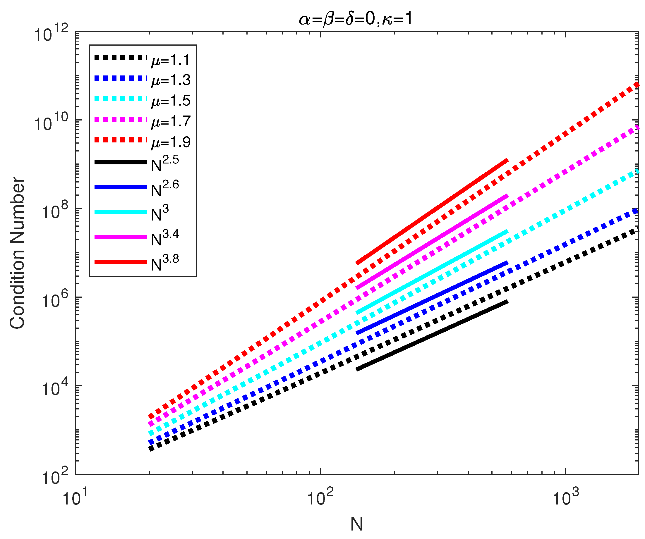
From the above Lemma, it is known that the first row of the DMLTCD is all zeros when $\delta >\mu$, and all infinity when $\delta <\mu$, so is the last row of the DMRTCD. In practice, the first row and column of the DMCHD (the DMRTCD) are removed according to initial or boundary value conditions. The DMLTCD (the DMRTCD) is full for every $\mu >0$, and the condition number of the DMLTCD (the DMRTCD) is like the first- or second-order differentiation matrix in the collocation method, as usual. We compute the condition numbers for different values of $\mu$ and show those in Figure 1 (for $0<\mu <1$) and Figure 2 (for $1<\mu <2$). The behavior of the condition number of the DMLTCD (the DMRTCD) is like $O\left(N^{2\mu }\right)$ from numerical tests.

Before providing more numerical results of tests, I would like to mention that all codes were compiled by using MatLab R2019a on pc with AMD Ryzen 7, 5800H with Radeon Graphics 3.20 GHz, RAM 16 G.

5. Applications to Nonlinear Initial Value Problems

Let $0<\mu <1$. In this section, we apply the spectral collocation method to the initial value problem of nonlinear fractional ordinary differential equation below:

$$\left\{\begin{array}{c}{}_0^C{\mathrm{D}}_x^{\mu ,\kappa }u\left(x\right)=f(x,u),0<x\le T,\hfill \\ u\left(0\right)=u_0.\hfill \end{array}\right.$$

(28)

Hereafter, we assume that $f(x,u)$ is continuous in the given domain and satisfies the Lipschitz condition with respect to the second variable, which guarantees the existence and uniqueness of the solution.

The spectral collocation method based on the TFJFs for (28) is to find $u_N\in {\mathbb{F}}_{N,l}^{\delta ,\kappa }$ such that

$${}_0^C{\mathrm{D}}_x^{\mu ,\tilde{\kappa }}{u}_N\left(x\right)=f(x,u_N\left(x\right)),x=x_j^{\alpha ,\beta }=\frac{T(1+{\xi }_j)}{2},j=1,2,\cdots ,N,$$

(29)

and

$$u_N\left(0\right)=u_0.$$

(30)

The above two equations lead to the following linear system

$${\left(\frac{2}{T}\right)}^{\mu }{\overline{\mathbf{D}}}_{s,l}^{\mu ,\tilde{\kappa }}\mathbf{u}=\mathbf{f}\left(\mathbf{u}\right),$$

(31)

where ${\overline{\mathbf{D}}}_{s,l}^{\mu ,\tilde{\kappa }}$ is the submatrix of ${\mathbf{D}}_{s,l}^{\mu ,\tilde{\kappa }}$, which deletes the first row and column of ${\mathbf{D}}_{s,l}^{\mu ,\tilde{\kappa }},\mathbf{u}=u_N\left(\mathbf{x}\right),\mathbf{f}\left(\mathbf{u}\right)=f(\mathbf{x},\mathbf{u})+u_a{\mathbf{d}}_0,\mathbf{x}={[x_1^{\alpha ,\beta },x_2^{\alpha ,\beta },\cdots ,x_N^{\alpha ,\beta }]}^T,{\mathbf{d}}_0$ the first column of ${\mathbf{D}}_{s,l}^{\mu ,\tilde{\kappa }}$.

We need to solve a nonlinear system (31) when f is nonlinear with respect to u. The iteration methods can be used, e.g., Newton method. To measure the accuracy of the method, we define the errors by

$$E_0=\underset{i=1,2,\cdots ,N}{max}\{|u\left(x_i\right)-u_N\left(x_i\right)|\},$$

where $u\left(x\right)$ and $u_N\left(x\right)$ are the exact and numerical solutions, respectively.

Example 1.

Consider (28) and $f(x,u)=g\left(x\right)-u^2$, where $g\left(x\right)$ is determined by

$$g\left(x\right)=u^2+{}_0^C{\mathrm{D}}_x^{\mu ,\kappa }u\left(x\right).$$

The following two cases of the exact solutions are considered [33]:

C1. 

$u\left(x\right)=e^{-\kappa x}(x^2-x)$ with $T=5$.

C2. 

$u\left(x\right)=e^{-\kappa x}\left(x^8-3x^{4+\mu /2}+\frac{9}{4}{x}^{\mu }\right)$ with $T=1.$

Clearly, the homogeneous initial condition $u\left(0\right)=0$ is fulfilled. In this example, the Newton method is applied to solving the nonlinear system (31), which takes the following form:

$${\mathbf{u}}^{n+1}={\mathbf{u}}^n+{\left(\mathbf{D}+2diag\left({\mathbf{u}}^n\right)\right)}^{-1}(\mathbf{D}{\mathbf{u}}^n+{\mathbf{u}}^n.\ast {\mathbf{u}}^n-\mathbf{g}),n=0,1,\cdots ,$$

where $\mathbf{g}={[g\left(x_1^{\alpha ,\beta }\right),g\left(x_2^{\alpha ,\beta }\right),\cdots ,g\left(x_N^{\alpha ,\beta }\right)]}^T$ and $\mathbf{D}={\left(\frac{2}{T}\right)}^{\mu }{\overline{\mathbf{D}}}_{s,l}^{\mu ,\tilde{\kappa }}$.

Since $u\left(x\right)\in {\mathbb{F}}_2^{0,\kappa }$, with two degrees of freedom ($N=2,\delta =0$), the method solves the problem C1 exactly without consideration of nonlinear approximation. It is noticed that the predictor–corrector method to solve the same problem in [33] achieves accuracy ${10}^{-4}$ by $h=1/160$, whilst our method achieves an accuracy ${10}^{-16}$ by $N=2$ (the iterative number is less than 8 in the Newton method).

For the exact solution $u\notin {\mathbb{F}}_N^{\delta ,\kappa }$ for any $\delta >-1$ in C2, we test different $N,\delta$ and apply the Newton method with maximum iterative step 20 to solve the nonlinear system. We list the error $E_0$ by $N=10,20,40,80,160$ and $\delta =\mu -1+5\ast {10}^{-11}$ for the case C2 in

Table 1. The numerical errors $E_0$ of Example 1 with C2 solution ($\alpha =0,\beta =0,\kappa =1$).

$\mathit{N}(1/\mathit{h})$	$\mathit{\mu }=0.2$ [33]	$\mathit{\mu }=0.2$	$\mathit{\mu }=0.5$ [33]	$\mathit{\mu }=0.5$	$\mathit{\mu }=0.9$ [33]	$\mathit{\mu }=0.9$
10	5.811 × 10${}^{-1}$	1.0898 × 10${}^{-7}$	2.441 × 10${}^{-2}$	8.4114 × 10${}^{-7}$	7.771 × 10${}^{-3}$	1.3961 × 10${}^{-6}$
20	2.001 × 10${}^{-1}$	5.1711 × 10${}^{-10}$	6.381 × 10${}^{-3}$	2.8558 × 10${}^{-9}$	1.441 × 10${}^{-3}$	3.3180 × 10${}^{-9}$
40	6.501 × 10${}^{-2}$	3.8736 × 10${}^{-13}$	2.821 × 10${}^{-3}$	7.4061 × 10${}^{-12}$	6.001 × 10${}^{-4}$	7.5808 × 10${}^{-12}$
80	8.351 × 10${}^{-3}$	1.2290 × 10${}^{-13}$	3.841 × 10${}^{-4}$	3.6507 × 10${}^{-13}$	1.521 × 10${}^{-4}$	1.1427 × 10${}^{-13}$
160	4.721 × 10${}^{-4}$	1.8164 × 10${}^{-11}$	2.231 × 10${}^{-5}$	1.5149 × 10${}^{-12}$	1.541 × 10${}^{-5}$	1.7109 × 10${}^{-13}$

. We also list the results by the predictor–corrector method to solve the same problem in [33]. It is shown our method is more superior.

6. Applications to the Fractional Helmholtz and Burgers Equations

6.1. Fractional Helmholtz Equation

Let $1<\mu <2$. In this subsection, we apply the spectral collocation method to the following fractional Helmholtz equation:

$$\left\{\begin{array}{c}{\lambda }^{2}u\left(x\right)-{}_a^C{\mathrm{D}}_x^{\mu ,\kappa }u\left(x\right)=f\left(x\right),a<x<b,\hfill \\ u\left(a\right)=u_a,u\left(b\right)=u_b.\hfill \end{array}\right.$$

(32)

The spectral collocation method based on the TFJFs for (32) is to find $u_N\in {\mathbb{F}}_N^{\delta ,\kappa }$ such that

$${\lambda }^2{u}_N\left(x\right)-{}_a^C{\mathrm{D}}_x^{\mu ,\kappa }{u}_N\left(x\right)=f\left(x\right),x=x_j^{\alpha ,\beta },j=1,2,\cdots ,N-1,$$

(33)

and

$$u_N\left(a\right)=u_a,u_N\left(b\right)=u_b.$$

(34)

The above two equations lead to the following linear system:

$$\left({\lambda }^2\mathbb{I}-{\left(\frac{2}{b-a}\right)}^{\mu }{\tilde{\mathbf{D}}}_{s,l}^{\mu ,\tilde{\kappa }}\right)\mathbf{u}=\mathbf{f},$$

(35)

where $\mathbb{I}$ is the unitary matrix, ${\tilde{\mathbf{D}}}_{s,l}^{\mu ,\tilde{\kappa }}$ is the inner part of ${\mathbf{D}}_{s,l}^{\mu ,\tilde{\kappa }}$, i.e., without the last row and column of ${\overline{\mathbf{D}}}_{s,l}^{\mu ,\tilde{\kappa }}$, $\mathbf{f}=f\left(\mathbf{x}\right)+u_a{\mathbf{d}}_0+u_b{\mathbf{d}}_N,$${\mathbf{d}}_0$ and ${\mathbf{d}}_N$ the first and last columns of ${\mathbf{D}}_{s,l}^{\mu ,\tilde{\kappa }}$.

To measure the accuracy of the method, we define the errors by

$$E_0\left(N\right)=\underset{i=1,\cdots ,N-1}{max}\{|u\left(x_i\right)-u_N\left(x_i\right)|\},$$

where $u\left(x\right)$ and $u_N\left(x\right)$ are exact and numerical solutions, respectively. To understand the convergence behavior of the method, we define the order of convergence by

$$Ord(N_1,N_2)=-\frac{log\left(E_0\left(N_1\right)\right)-log\left(E_0\left(N_2\right)\right)}{log\left(N_1\right)-log\left(N_2\right)}.$$

Example 2.

Consider (32) with $[a,b]=[0,2]$. The source term $f\left(x\right)$ is chosen such that the problem satisfies one of the following two cases:

C1. 

Smooth solution: $u\left(x\right)=e^{-\kappa x}sin\left(\pi x\right)$.

C2. 

Solution with low regularity: $u\left(x\right)=e^{-\kappa x}\left[2^{\sigma +1}{x}^{\sigma }-x^{2\sigma +1}\right]$.

The homogeneous boundary conditions are implemented for two cases. The term ${}_a^C{\mathrm{D}}_x^{\mu ,\kappa }u\left(x\right)$ in C1 is approximated by

$${}_0^C{\mathrm{D}}_x^{\mu ,\kappa }{e}^{-\kappa x}sin\left(\pi x\right)\approx e^{-\kappa x}\sum _{k=1}^L\frac{{(-1)}^k{\pi }^{2k+1}}{\Gamma (2k+2-\mu )}{x}^{2k+1-\mu },$$

with $L=50$ to compute the right-hand function (RHF) $f\left(x\right)$.

For the smooth solution C1, we solve Equation (32) by $\delta =0$. We list the errors $E_0$ in

Table 2. Errors $E_0$ of Example 2 with solution C1 ($\alpha =\beta =0,\delta =0,\kappa =1,\lambda =0$).

N	$\mathit{\mu }=1.1$	$\mathit{\mu }=1.3$	$\mathit{\mu }=1.5$	$\mathit{\mu }=1.7$	$\mathit{\mu }=1.9$	$\mathit{\mu }=1.99$
4	1.781 × 10${}^{-1}$	1.191 × 10${}^{-1}$	9.844 × 10${}^{-2}$	1.091 × 10${}^{-1}$	9.028 × 10${}^{-2}$	4.519 × 10${}^{-2}$
8	5.110 × 10${}^{-4}$	3.488 × 10${}^{-4}$	2.818 × 10${}^{-4}$	2.931 × 10${}^{-4}$	2.610 × 10${}^{-4}$	4.833 × 10${}^{-5}$
12	2.173 × 10${}^{-7}$	1.373 × 10${}^{-7}$	1.016 × 10${}^{-7}$	1.448 × 10${}^{-7}$	1.699 × 10${}^{-7}$	3.235 × 10${}^{-8}$
16	2.618 × 10${}^{-11}$	1.550 × 10${}^{-11}$	1.160 × 10${}^{-11}$	1.732 × 10${}^{-11}$	2.501 × 10${}^{-11}$	5.182 × 10${}^{-12}$
20	1.200 × 10${}^{-14}$	1.299 × 10${}^{-14}$	1.241 × 10${}^{-14}$	1.474 × 10${}^{-14}$	1.302 × 10${}^{-14}$	1.258 × 10${}^{-14}$

,

Table 3. Errors $E_0$ of Example 2 with solution C1 ($\mu =1.4,\delta =0,\kappa =5,\lambda =2$).

N	$\mathit{\alpha }=\mathit{\beta }=0$	$\mathit{\alpha }=\mathit{\beta }=-0.5$	$\mathit{\alpha }=-\mathit{\beta }=0.5$	$(\mathit{\alpha },\mathit{\beta })=\left(-0.3,0.8\right)$	$\mathit{\alpha }=\mathit{\beta }=1$
4	2.282 × 10${}^{-2}$	2.901 × 10${}^{-2}$	1.322 × 10${}^{-2}$	2.338 × 10${}^{-2}$	1.605 × 10${}^{-2}$
8	9.931 × 10${}^{-5}$	5.828 × 10${}^{-5}$	2.701 × 10${}^{-5}$	3.397 × 10${}^{-4}$	1.821 × 10${}^{-4}$
12	3.315 × 10${}^{-8}$	2.504 × 10${}^{-8}$	1.210 × 10${}^{-8}$	1.889 × 10${}^{-7}$	1.075 × 10${}^{-7}$
16	3.008 × 10${}^{-12}$	2.379 × 10${}^{-12}$	1.493 × 10${}^{-12}$	2.353 × 10${}^{-11}$	1.419 × 10${}^{-11}$
20	1.174 × 10${}^{-14}$	2.498 × 10${}^{-15}$	1.443 × 10${}^{-15}$	1.282 × 10${}^{-14}$	2.776 × 10${}^{-14}$

and

Table 4. Errors $E_0$ of Example 2 with solution C1 ($\mu =1.6,\alpha =\beta =0,\delta =0,\lambda =1000$).

N	$\mathit{\kappa }=1$	$\mathit{\kappa }=2$	$\mathit{\kappa }=3$	$\mathit{\kappa }=5$	$\mathit{\kappa }=8$	$\mathit{\kappa }=10$
4	2.131 × 10${}^{-6}$	1.509 × 10${}^{-6}$	1.068 × 10${}^{-6}$	5.353 × 10${}^{-7}$	1.900 × 10${}^{-7}$	9.521 × 10${}^{-8}$
8	3.355 × 10${}^{-8}$	3.035 × 10${}^{-8}$	2.745 × 10${}^{-8}$	2.247 × 10${}^{-8}$	1.663 × 10${}^{-8}$	1.361 × 10${}^{-8}$
12	3.806 × 10${}^{-11}$	3.632 × 10${}^{-11}$	3.467 × 10${}^{-11}$	3.158 × 10${}^{-11}$	2.745 × 10${}^{-11}$	2.500 × 10${}^{-11}$
16	9.076 × 10${}^{-15}$	8.868 × 10${}^{-15}$	8.618 × 10${}^{-15}$	8.188 × 10${}^{-15}$	7.522 × 10${}^{-15}$	7.119 × 10${}^{-15}$
20	2.220 × 10${}^{-16}$	1.110 × 10${}^{-16}$	1.110 × 10${}^{-16}$	5.551 × 10${}^{-17}$	2.082 × 10${}^{-17}$	2.776 × 10${}^{-17}$

for different values of parameters $\mu ,\alpha ,\beta ,\kappa$ and $\lambda$, which show that spectral accuracy can be achieved for a large range of parameters. It is observed that there is no significant difference between the Chebyshev method ($\alpha =\beta =-0.5$) and the Legendre method ($\alpha =\beta =0$) or other Jacobi methods by precision (see Table 3).

The exact solution has low regularity when $\sigma$ is a non-integer in C2, so we expect the order of convergence of our method to be finite. We list the errors $E_0$ and the order of convergence $Ord$ in

Table 5. Errors $E_0$ and $Ord$ of Example 2 with solution C2 ($\sigma =1.4,\alpha =\beta =0,\delta =0,\kappa =1,\lambda =1$).

	$\mathit{\mu }=1.1$		$\mathit{\mu }=1.3$		$\mathit{\mu }=1.5$		$\mathit{\mu }=1.9$
$\mathit{N}$	${\mathit{E}}_{\mathbf{0}}$	Ord	${\mathit{E}}_{\mathbf{0}}$	Ord	${\mathit{E}}_{\mathbf{0}}$	Ord	${\mathit{E}}_{\mathbf{0}}$	Ord
8	3.744 × 10${}^{-2}$	-	4.300 × 10${}^{-2}$	-	4.544 × 10${}^{-2}$	-	2.319 × 10${}^{-2}$	-
16	6.835 × 10${}^{-3}$	2.45	8.416 × 10${}^{-3}$	2.35	1.331 × 10${}^{-2}$	1.77	1.350 × 10${}^{-2}$	0.78
32	1.072 × 10${}^{-3}$	2.67	1.877 × 10${}^{-3}$	2.16	3.968 × 10${}^{-3}$	1.75	7.138 × 10${}^{-3}$	0.92
64	1.607 × 10${}^{-4}$	2.74	4.121 × 10${}^{-4}$	2.19	1.150 × 10${}^{-3}$	1.79	3.632 × 10${}^{-3}$	0.97
128	2.482 × 10${}^{-5}$	2.69	8.961 × 10${}^{-5}$	2.20	3.327 × 10${}^{-4}$	1.79	1.829 × 10${}^{-3}$	0.99
256	3.946 × 10${}^{-6}$	2.65	1.950 × 10${}^{-5}$	2.20	9.585 × 10${}^{-5}$	1.80	9.166 × 10${}^{-4}$	1.00
512	6.369 × 10${}^{-7}$	2.63	4.245 × 10${}^{-6}$	2.20	2.757 × 10${}^{-5}$	1.80	4.588 × 10${}^{-4}$	1.00

,

Table 6. Errors $E_0$ and $Ord$ of Example 2 with solution C2 ($\sigma =1.4,\alpha =\beta =0,\delta =0.4,\kappa =1,\lambda =1$).

	$\mathit{\mu }=1.1$		$\mathit{\mu }=1.3$		$\mathit{\mu }=1.5$		$\mathit{\mu }=1.9$
$\mathit{N}$	${\mathit{E}}_{\mathbf{0}}$	Ord	${\mathit{E}}_{\mathbf{0}}$	Ord	${\mathit{E}}_{\mathbf{0}}$	Ord	${\mathit{E}}_{\mathbf{0}}$	Ord
8	4.526 × 10${}^{-5}$	-	1.453 × 10${}^{-5}$	-	9.694 × 10${}^{-6}$	-	5.743 × 10${}^{-6}$	-
16	5.361 × 10${}^{-7}$	6.40	1.066 × 10${}^{-7}$	7.09	5.753 × 10${}^{-8}$	7.40	3.732 × 10${}^{-8}$	7.27
32	1.061 × 10${}^{-8}$	5.66	7.197 × 10${}^{-10}$	7.21	3.757 × 10${}^{-10}$	7.26	2.171 × 10${}^{-10}$	7.43
64	1.072 × 10${}^{-10}$	6.63	4.430 × 10${}^{-12}$	7.34	2.126 × 10${}^{-12}$	7.47	1.183 × 10${}^{-12}$	7.52
128	7.944 × 10${}^{-14}$	10.40	6.140 × 10${}^{-14}$	6.17	5.207 × 10${}^{-14}$	5.35	4.952 × 10${}^{-14}$	4.58

,

Table 7. Errors $E_0$ and $Ord$ of Example 2 with solution C2 ($\mu =1.4,\alpha =\beta =0,\delta =0,\kappa =1,\lambda =1$).

	$\mathit{\sigma }=1.2$		$\mathit{\sigma }=1.6$		$\mathit{\sigma }=1.9$		$\mathit{\sigma }=2.4$
$\mathit{N}$	${\mathit{E}}_{\mathbf{0}}$	Ord	${\mathit{E}}_{\mathbf{0}}$	Ord	${\mathit{E}}_{\mathbf{0}}$	Ord	${\mathit{E}}_{\mathbf{0}}$	Ord
8	8.700 × 10${}^{-2}$	-	2.008 × 10${}^{-2}$	-	2.608 × 10${}^{-3}$	-	2.659 × 10${}^{-3}$	-
16	2.745 × 10${}^{-2}$	1.66	3.490 × 10${}^{-3}$	2.52	2.875 × 10${}^{-4}$	3.18	1.369 × 10${}^{-4}$	4.28
32	9.543 × 10${}^{-3}$	1.52	6.934 × 10${}^{-4}$	2.33	3.740 × 10${}^{-5}$	2.94	8.736 × 10${}^{-6}$	3.97
64	3.160 × 10${}^{-3}$	1.59	1.317 × 10${}^{-4}$	2.40	4.672 × 10${}^{-6}$	3.00	5.404 × 10${}^{-7}$	4.01
128	1.049 × 10${}^{-3}$	1.59	2.509 × 10${}^{-5}$	2.39	5.866 × 10${}^{-7}$	2.99	3.380 × 10${}^{-8}$	4.00
256	3.468 × 10${}^{-4}$	1.60	4.768 × 10${}^{-6}$	2.40	7.357 × 10${}^{-8}$	3.00	2.120 × 10${}^{-9}$	3.99
512	1.145 × 10${}^{-4}$	1.60	9.050 × 10${}^{-7}$	2.40	9.206 × 10${}^{-9}$	3.00	1.476 × 10${}^{-10}$	3.84

and

Table 8. Errors $E_0$ and $Ord$ of Example 2 with solution C2 ($\mu =1.33,\alpha =\beta =0,\delta =\sigma -1,\kappa =2,\lambda =1$).

	$\mathit{\sigma }=1.2$		$\mathit{\sigma }=1.6$		$\mathit{\sigma }=1.9$		$\mathit{\sigma }=2.4$
$\mathit{N}$	${\mathit{E}}_{\mathbf{0}}$	Ord	${\mathit{E}}_{\mathbf{0}}$	Ord	${\mathit{E}}_{\mathbf{0}}$	Ord	${\mathit{E}}_{\mathbf{0}}$	Ord
8	1.163 × 10${}^{-5}$	-	1.331 × 10${}^{-5}$	-	1.202 × 10${}^{-5}$	-	1.302 × 10${}^{-5}$	-
16	1.165 × 10${}^{-7}$	6.64	9.526 × 10${}^{-8}$	7.13	6.495 × 10${}^{-8}$	7.53	7.022 × 10${}^{-8}$	7.53
32	1.180 × 10${}^{-9}$	6.63	6.321 × 10${}^{-10}$	7.24	3.020 × 10${}^{-10}$	7.75	4.644 × 10${}^{-10}$	7.24
64	1.122 × 10${}^{-11}$	6.72	3.846 × 10${}^{-12}$	7.36	1.316 × 10${}^{-12}$	7.84	1.643 × 10${}^{-11}$	4.82
128	1.047 × 10${}^{-13}$	6.74	5.762 × 10${}^{-14}$	6.06	5.529 × 10${}^{-14}$	4.57	1.715 × 10${}^{-13}$	6.58

. A possible guess of the $Ord$ for the case C2 with $\delta =0$ is $O\left(N^{-2(\sigma -\mu +1)}\right)$ from the results in Table 5 and Table 7. When $\delta =\sigma -1$, the super convergence can be observed; see the results in Table 6 and Table 8.

6.2. Fractional Burgers Equation

In the current subsection, we employ the spectral collocation method to solve the fractional Burgers equation (FBE)

$${\partial }_{t}u(x,t)+u(x,t){\partial }_{x}u(x,t)=ϵ{}_a^C{\mathrm{D}}_x^{\mu ,\kappa }u(x,t),$$

(36)

subject to homogeneous Dirichlet boundary conditions and initial condition $u(x,0)=u_0\left(x\right)$, where $ϵ>0$ and $1<\mu <2,(x,t)\in (a,b)\times (0,1]$.

For time advancing, we employ a semi-implicit time-discretization scheme, namely, the two-step second-order Crank-Nicolson/leapfrog scheme. Then, the full discretization scheme reads as

$$\left\{\begin{array}{cc}(\mathbb{I}-ϵ\tau \tilde{\mathbf{D}}){\mathbf{u}}^{n+1}=(\mathbb{I}+ϵ\tau \tilde{\mathbf{D}}){\mathbf{u}}^{n-1}-2\tau \left(diag\left({\mathbf{u}}^n\right)\mathbf{D}\right){\mathbf{u}}^n,\hfill & n\ge 1,\hfill \\ {\mathbf{u}}^1=(\mathbb{I}+ϵ\tau \tilde{\mathbf{D}}){\mathbf{u}}^0-\tau \left(diag\left({\mathbf{u}}^0\right)\mathbf{D}\right){\mathbf{u}}^0,\hfill \\ {\mathbf{u}}^0=u_0\left(\mathbf{x}\right),\hfill \end{array}\right.$$

(37)

where $\mathbf{D}$ is the first-order differentiation matrix and $\tilde{\mathbf{D}}={\left(\frac{2}{b-a}\right)}^{\mu }{\tilde{\mathbf{D}}}_{s,l}^{\mu ,\kappa }$.

Example 3.

Consider (36) with the initial profile as one of the following:

C1. 

$u_0\left(x\right)=sin\left(\pi x\right),x\in [-1,1].$

C2. 

$u_0\left(x\right)=e^{-4x^2},x\in [-6,6].$

In the example, we always take $\alpha =\beta =0,\tau ={10}^{-3}.$

We first consider the initial profile with two peaks, i.e., case C1. We show the numerical solutions of the FBE at time $t=1$ in Figure 3 for different values $N=50,100,300$ by $\mu =1.18,ϵ=1$ and $\kappa =0,1$ ($\kappa =0$ for non-tempered and $\kappa =1$ for tempered case). It is observed that the numerical solution is in good agreement with each other. The surface of the numerical solution for $\mu =1.4,\kappa =1,ϵ=1$ is plotted in Figure 4 with $N=200.$ The evolution of the numerical solution is observed. The numerical solutions of the FBE at time $t=1$ are plotted for different values of fractional-order $\mu =1.2,1.3,1.5,1.7,1.9$ and $\kappa =1,ϵ=1$ in Figure 5 and for different values of tempered factor $\kappa =0,0.5,1,1.5,2$ and $\mu =1.55,ϵ=1$ in Figure 6. We observed that the tempered diffusion becomes slower with larger $\kappa$.

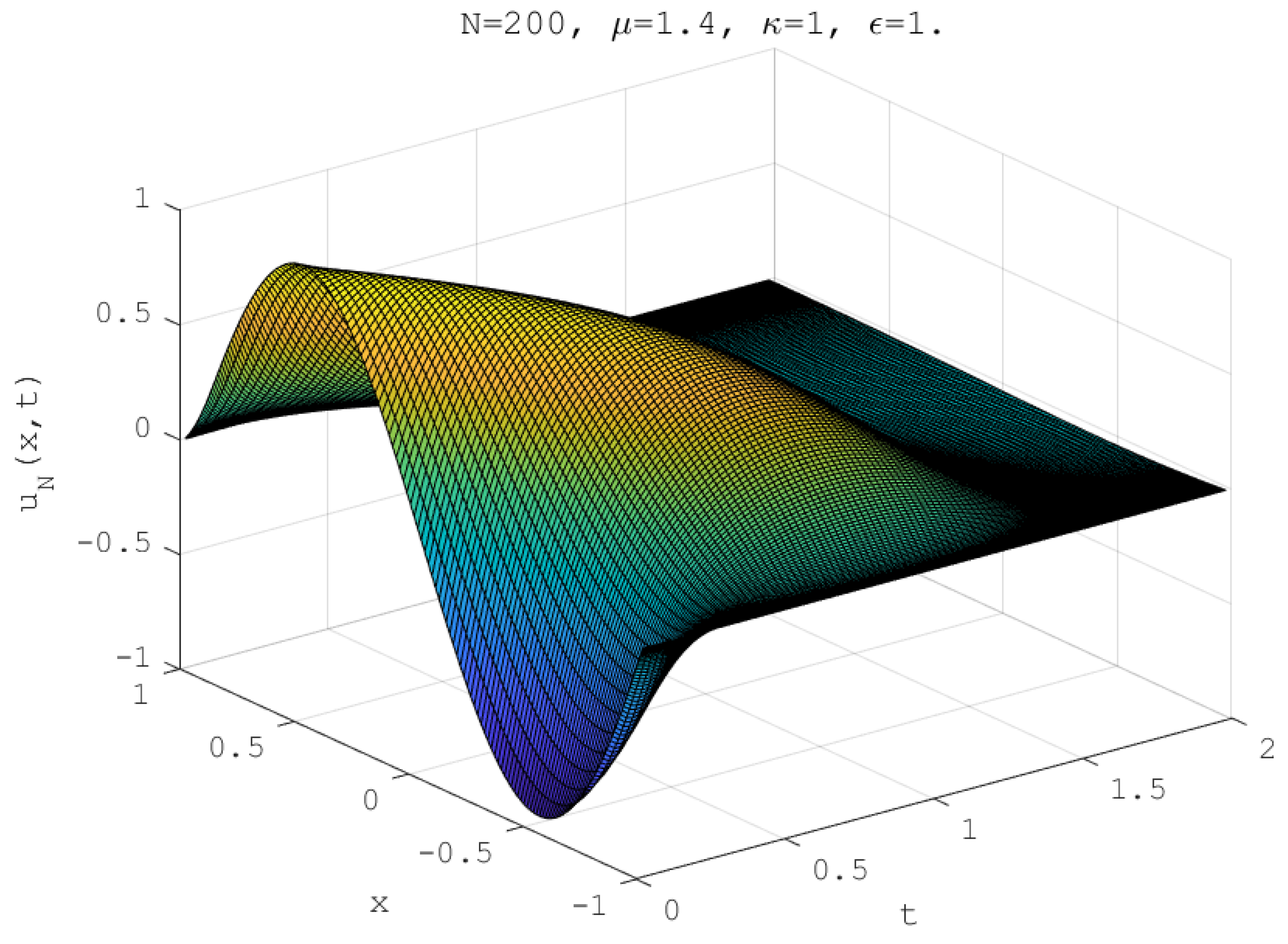
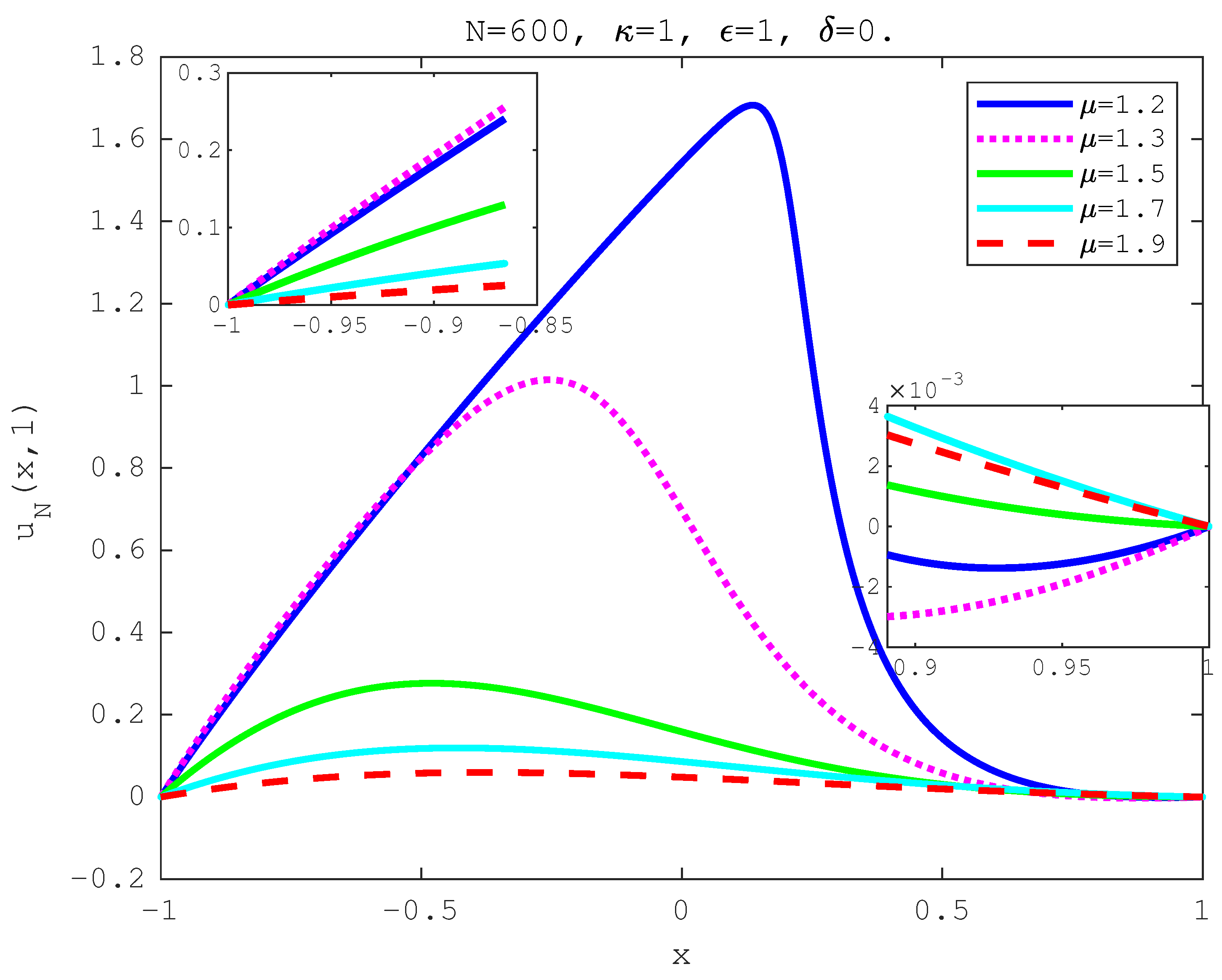
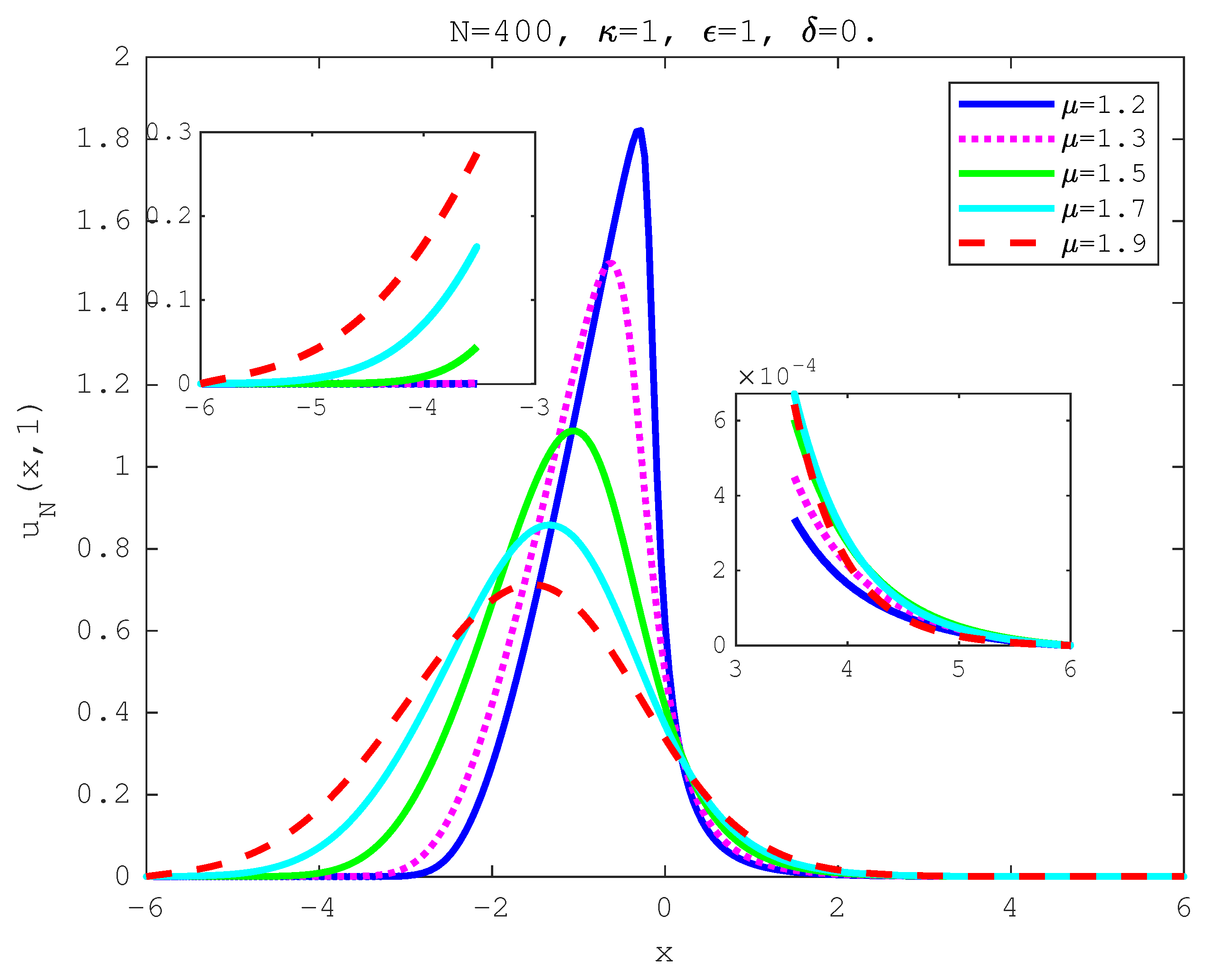
We consider the initial profile with single peak of case C2. We show the surface of the numerical solution for $\mu =1.4,\kappa =1,ϵ=1$ in Figure 7 and the evolution of the numerical solution. The numerical solutions of the FBE at time $t=1$ are plotted in Figure 8 for different values of fractional-order $\mu =1.2,1.3,1.5,1.7,1.9$ where $\kappa =1,ϵ=1$ and in Figure 9 for different values of tempered factor $\kappa =0,0.5,1,1.5,2$ where $\mu =1.55,ϵ=1$. It is shown that our method is a powerful tool to simulate the fractional-order diffusion of the Caputo derivative as well as of the tempered case.

7. Conclusions

Tempered fractional calculus is of importance in the family of fractional calculi with potential applications. In this paper, we present a spectral collocation method using the TFJFs as basis functions and obtain an efficient algorithm to solve tempered fractional differential equations. The key in implementing it is to stably evaluate the collocation differentiation matrix by utilizing a recurrence relation. The method is the direct collocation method in strong form and shares spectral accuracy when the solutions of FDEs are smooth from the approximate properties of the TFJFs. The effectiveness of the derived method is confirmed by numerical tests for the nonlinear initial problems, the fractional Helmholtz equation, and the fractional Burgers equation with the tempered Caputo derivative.

The method can be applied to other kinds of tempered fractional linear or nonlinear differential equations and even for the variable-order case. On the other hand, the method can be generalized to the multi-domain case, such as that in [34]. We will develop its further applications in the future. Meanwhile, the symmetries of the FD equations are also an interesting topic [35] that can be used to construct a structure-preserving high-order algorithm. We expect to consider it in the future.

The present method is not able to resolve directly the fractional derivative of more generalized fractal fractional derivatives, such as that in [36]. We will improve our method to tackle it in the future.

References

- Baeumera, B.; Meerschaert, M.M. Tempered stable Levy motion and transient super-diffusion. J. Comput. Appl. Math. 2010, 233, 2438–2448. [Google Scholar] [CrossRef] [Green Version]
- Sabzikar, F.; Meerschaerta, M.M.; Chen, J.H. Tempered fractional calculus. J. Comput. Phys. 2015, 293, 14–28. [Google Scholar] [CrossRef] [PubMed] [Green Version]
- Sibatov, R.T.; Sun, H.G. Tempered fractional equations for quantum transport in mesoscopic one-dimensional systems with fractal disorder. Fractal Fract. 2019, 3, 47. [Google Scholar] [CrossRef] [Green Version]
- Wang, H.H.; Li, C. Fast difference scheme for a tempered fractional Burgers equation in porous media. Appl. Math. Lett. 2022, 132, 108143. [Google Scholar] [CrossRef]
- Meerschaert, M.M.; Zhang, Y.; Baeumer, B. Tempered anomalous diffusion in heterogeneous systems. Geophys. Res. Lett. 2008, 35, L17403. [Google Scholar] [CrossRef]
- Meerschaert, M.M.; Sabzikar, F.; Phanikumar, M.; Zeleke, A. Tempered fractional time series model for turbulence in geophysical flows. J. Stat. Mech. Theory Exp. 2014, 14, 1742–5468. [Google Scholar] [CrossRef] [Green Version]
- Li, C.; Deng, W.H. High order schemes for the tempered fractional diffusion equations. Adv. Comput. Math. 2016, 42, 543–572. [Google Scholar] [CrossRef] [Green Version]
- Deng, W.H.; Zhang, Z.J. Variational formulation and efficient implementation for solving the tempered fractional problems. Numer. Methods Part. Diff. Eqns. 2018, 34, 1224–1257. [Google Scholar] [CrossRef] [Green Version]
- Chen, M.H.; Deng, W.H. A second-order accurate numerical method for the space-time tempered fractional diffusion-wave equation. Appl. Math. Lett. 2017, 68, 87–93. [Google Scholar] [CrossRef]
- Ding, H.F.; Li, C.P. A high-order algorithm for time-Caputo-tempered partial differential equation with Riesz derivatives in two spatial dimensions. J. Sci. Comput. 2019, 80, 81–109. [Google Scholar] [CrossRef]
- Guo, L.; Zeng, F.H.; Turner, I.; Burrage, K.; Karniadakis, G.E. Efficient multistep methods for tempered fractional calculus: Algorithms and simulations. SIAM J. Sci. Comput. 2019, 41, A2510–A2535. [Google Scholar] [CrossRef] [Green Version]
- Cao, J.L.; Xiao, A.G.; Bu, W.P. Finite difference/finite element method for tempered time fractional advection-dispersion equation with fast evaluation of Caputo derivative. J. Sci. Comput. 2020, 83, 48. [Google Scholar] [CrossRef]
- Sun, X.R.; Li, C.; Zhao, F.Q. Local discontinuous Galerkin methods for the time tempered fractional diffusion equation. Appl. Math. Comput. 2020, 365, 124725. [Google Scholar] [CrossRef] [Green Version]
- Safari, Z.; Loghmani, G.B.; Ahmadinia, M. Convergence analysis of a LDG method for time-space tempered fractional diffusion equations with weakly singular solutions. J. Sci. Comput. 2022, 91, 68. [Google Scholar] [CrossRef]
- Bu, L.L.; Oosterlee, C.W. On a multigrid method for tempered fractional diffusion equations. Fractal Fract. 2021, 5, 145. [Google Scholar] [CrossRef]
- Çelik, C.; Duman, M. Finite element method for a symmetric tempered fractional diffusion equation. Appl. Numer. Math. 2017, 120, 270–286. [Google Scholar] [CrossRef]
- Zayernouri, M.; Ainsworth, M.; Karniadakis, G.E. Tempered fractional Sturm-Liouville eigenproblems. SIAM J. Sci. Comput. 2015, 37, A1777–A1800. [Google Scholar] [CrossRef] [Green Version]
- Hanert, E.; Piret, C. A Chebyshev pseudospectral method to solve the space-time tempered fractional diffusion equation. SIAM J. Sci. Comput. 2015, 36, A1797–A1812. [Google Scholar] [CrossRef]
- Chen, S.; Shen, J.; Wang, L.L. Laguerre functions and their applications to tempered fractional differential equations on infinite intervals. J. Sci. Comput. 2018, 74, 1286–1313. [Google Scholar] [CrossRef]
- Luo, W.H.; Gu, X.M.; Yang, L.; Meng, J. A Lagrange-quadratic spline optimal collocation method for the time tempered fractional diffusion equation. Math. Comput. Simulat. 2021, 182, 1–24. [Google Scholar] [CrossRef]
- Moghaddam, B.P.; Machado, J.A.T.; Babaei, A. A computationally efficient method for tempered fractional differential equations with application. Comp. Appl. Math. 2018, 37, 3657–3671. [Google Scholar] [CrossRef]
- Liemert, A.; Kienle, A. Computational solutions of the tempered fractional wave-diffusion equation. Fract. Calc. Appl. Aanl. 2017, 20, 139–158. [Google Scholar] [CrossRef]
- Li, C.; Deng, W.H.; Zhao, L.J. Well-posedness and numerical algorithm for the tempered fractional ordinary differential equations. Disc. Cont. Dyn. Sys. B 2019, 24, 1989–2015. [Google Scholar]
- Deng, W.H.; Li, B.Y.; Tian, W.Y.; Zhang, P.W. Boundary problems for the fractional and tempered fractional operators. Multiscale Model. Simul. 2018, 16, 125–149. [Google Scholar] [CrossRef] [Green Version]
- Fahad, H.M.; Fernandez, A.; Rehman, M.U.; Siddiqi, M. Tempered and Hadamard-Type fractional calculus with respect to functions. Mediterr. J. Math. 2021, 18, 143. [Google Scholar] [CrossRef]
- Chen, M.H.; Deng, W.H. High order algorithms for the fractional substantial diffusion equation with truncated Lévy flights. SIAM J. Sci. Comput. 2015, 37, A890–A917. [Google Scholar] [CrossRef] [Green Version]
- Huang, C.; Zhang, Z.M.; Song, Q.S. Spectral method for substantial fractional differential equations. J. Sci. Comput. 2018, 74, 1554–1574. [Google Scholar] [CrossRef]
- Chen, S.; Shen, J.; Wang, L.L. Generalized Jacobi functions and their applications to fractional differential equations. Math. Comput. 2016, 85, 1603–1638. [Google Scholar] [CrossRef] [Green Version]
- Wu, X.C.; Deng, W.H.; Barkai, E. Tempered fractional Feynman-Kac equation: Theory and examples. Phys. Rev. E 2016, 93, 032151. [Google Scholar] [CrossRef] [Green Version]
- Shen, J.; Tang, T.; Wang, L.L. Spectral Methods: Algorithms, Analysis and Applications; Springer: Berlin/Heidelberg, Germany, 2011. [Google Scholar]
- Szegö, G. Orthogonal Polynomials, 4th ed.; American Mathematical Society: Providence, RI, USA, 1975. [Google Scholar]
- Liu, W.J.; Wang, L.L.; Wu, B.Y. Optimal error estimates for Legendre expansions of singular functions with fractional derivatives of bounded variation. Adv. Comput. Math. 2021, 47, 79. [Google Scholar] [CrossRef]
- Deng, J.W.; Zhao, L.J.; Wu, Y.J. Fast predictor-corrector approach for the tempered fractional differential equations. Numer. Algor. 2017, 74, 717–754. [Google Scholar] [CrossRef]
- Zhao, T.G.; Mao, Z.P.; Karniadakis, G.E. Multi-domain spectral collocation method for variable-order nonlinear fractional differential equations. Comput. Methods Appl. Mech. Eng. 2019, 348, 377–395. [Google Scholar] [CrossRef] [Green Version]
- Zhou, Y.; Zhang, Y. Noether symmetries for fractional generalized Birkhoffian systems in terms of classical and combined Caputo derivatives. Acta Mech. 2020, 231, 3017–3029. [Google Scholar] [CrossRef]
- Youssri, Y.H.; Atta, A.G. Spectral collocation approach via normalized shifted Jacobi polynomials for the nonlinear Lane-Emden equation with fractal-fractional derivative. Fractal Fract. 2023, 7, 133. [Google Scholar] [CrossRef]
Figure 1.
Condition number of DMLTCD with .
Figure 2.
Figure 3.
Numerical solution for Example 3 of with .
Figure 4.
Figure 5.
Figure 6.
Figure 7.
Figure 8.
Figure 9.