1. Introduction
In recent years, many new machine learning (ML) algorithms have been developed that can analyze and model data obtained from two-dimensional signals [
1,
2,
3,
4]. Many of these algorithms are based on supervised machine learning (SML) techniques such as binomial logistic regression, decision trees, support vector machines, and artificial neural networks [
5,
6,
7]. These techniques and the resulting sensing systems have the potential to greatly improve image recognition and classification in various biological and medical fields. The use of SML for analyzing microscopic data in histology, pathology, and cell biology is a relatively new area of research, but it holds great promise for being integrated into future diagnostic protocols and procedures. Additionally, AI can automate and speed up decision-making in these fields by quickly processing large amounts of data. Furthermore, some supervised machine learning models may be able to detect patterns in microscopic data related to tissue and cell structure that are not visible to even the most experienced professionals [
8,
9,
10,
11,
12].
There are many ways to train and test a machine learning model applicable to microscopy. RGB (red, green, blue) pixel intensities obtained from micrographs in JPG and BMP formats can sometimes be used as input data for AI training, such as in convolutional neural networks [
13,
14,
15]. Another way is to perform a two-dimensional signal analysis and obtain a set of quantifications that are used as inputs. Recently different forms of texture analysis were suggested as an objective and efficient way to generate these quantifications that can be used for machine learning. An example would be gray-level co-occurrence matrix (GLCM) analysis, where pairs of resolution units with the assigned gray-level intensity quantifications are analyzed using second-order statistics [
1,
16,
17,
18]. This way, several important textural features can be calculated, such as angular second moment as an indicator of textural uniformity or inverse difference moment as an indicator of local homogeneity. Approaches based on GLCM have been used on numerous occasions to detect subtle morphological alterations in cells and tissues in various experimental settings, both in vivo and in vitro. It was suggested that GLCM as a method may detect changes in nuclear chromatin following the induction of cell damage. Sometimes, discrete wavelet transform (DWT), as a form of mathematical image analysis, is used as an addition to GLCM to provide useful insight into the changes in GLCM features [
1,
18]. Both GLCM and DWT indicators can be utilized to develop a machine learning model for the classification of microscopic phenomena or for predicting pathological processes.
Fractal analysis of microscopic data is also a way to obtain quantifications for machine learning that can later be used for classification or prediction. Fractal analysis enables us to indirectly measure the complexity of a signal, typically by determining the fractal dimension value. This technique is often used in microscopy in binarized or grayscale images of biological structures and can sometimes be useful in evaluating different regions of interest (ROIs) in micrographs representing parts of tissue or cellular components. Fractal analysis of nuclear structure was shown to be a potentially useful predictor of some pathological processes, with fractal dimension also being a potentially valuable prognostic indicator for the outcome of some diseases [
19,
20,
21].
Osmotic stress is a potentially important contributing factor to the development of many diseases, particularly the ones associated with inflammation [
22]. Protective biochemical responses and signaling pathways that are activated as the result of osmotic stress, although not entirely understood, are present in almost all organisms. Mild stress in some cells usually does not lead to substantial and microscopically-visible morphological changes; however, this does not necessarily imply that the cell remains structurally and functionally intact [
23,
24,
25]. So far, to the best of our knowledge, fractal, GLCM, and wavelet analyses have not been used for the development of a computer sensing system capable of evaluating morphological changes associated with osmotic stress. Recently, machine learning models have been developed on several occasions for the prediction and classification of various physiological and pathological phenomena associated with osmotic stress. Some examples would be the prediction of ethanol yields in yeast fermentation cultures during high-sugar osmotic stress [
26] or the classification of electrophysiological responses resulting from such stress in plants [
27]. However, none of these or similar machine learning methods used fractal, GLCM, and wavelet data as inputs.
Our research presented in this article indicates that exposure of yeast cells to hyperosmotic stress causes notable alterations in the GLCM, fractal, and wavelet parameters of their nuclear structure. We also demonstrate that it is possible to use these indicators as input data for machine learning models, such as the ones based on random forest and support vector machine algorithms, to identify cells that have been exposed to hyperosmotic stress with acceptable accuracy. These findings provide a foundation for initiating the development of AI-based techniques that leverage GLCM, fractal, and wavelet data to distinguish between damaged and healthy cells and to forecast diverse physiological and pathological phenomena linked with osmotic stress.
2. Materials and Methods
Saccharomyces cerevisiae yeast cells similar to the ones described previously [
8], previously purchased from commercially available sources, were kept in Yeast Extract Peptone–Dextrose (YPD) broth in an orbital shaker at 25 °C and pH 6.5 ± 0.2 with agitation at 200 rpm. The cell samples for the experiments were later transferred to special tissue chamber/slides, as mentioned in our previous publication [
8]. The genetic information of Saccharomyces cerevisiae—a widely studied microorganism in molecular genetics and cell biology—can be found at The European Nucleotide Archive. The cells were exposed to a hyperosmotic environment by adding NaCl to reach 0.8 M concentration for 2 h, after which normal tonicity was swiftly restored. We created digital micrographs of the treated and control cells in JPG format using a TCA1000-C instrument equipped with an Aptina MT9J003 CMOS sensor mounted on OPTIC900TH Trinocular Biological Microscope (COLO LabExperts, Novo Mesto, Slovenia). The size of the micrographs was set to 3584 (width) × 2748 (height) resolution units, and the bit depth equaled 24. A similar approach was applied in our previously published work [
8], although, in our study, we modified the values of color temperature, saturation, hue and other parameters in order to make the micrographs even more suitable for GLCM analysis. The micrographs were converted to an 8-bit grayscale format for the calculation of GLCM parameters.
For GLCM evaluation, we used our modification of plugins previously developed by Julio E. Cabrera and Toby C. Cornish for the ImageJ software (National Institutes of Health, Bethesda, MD, USA, version 1.53e based on 64-bit Java 1.8.0_172). We analyzed a total of 2000 circular nuclear regions of interest (ROI): 1000 ROIs of the cells exposed to a hyperosmotic environment and 1000 ROIs from control cells (
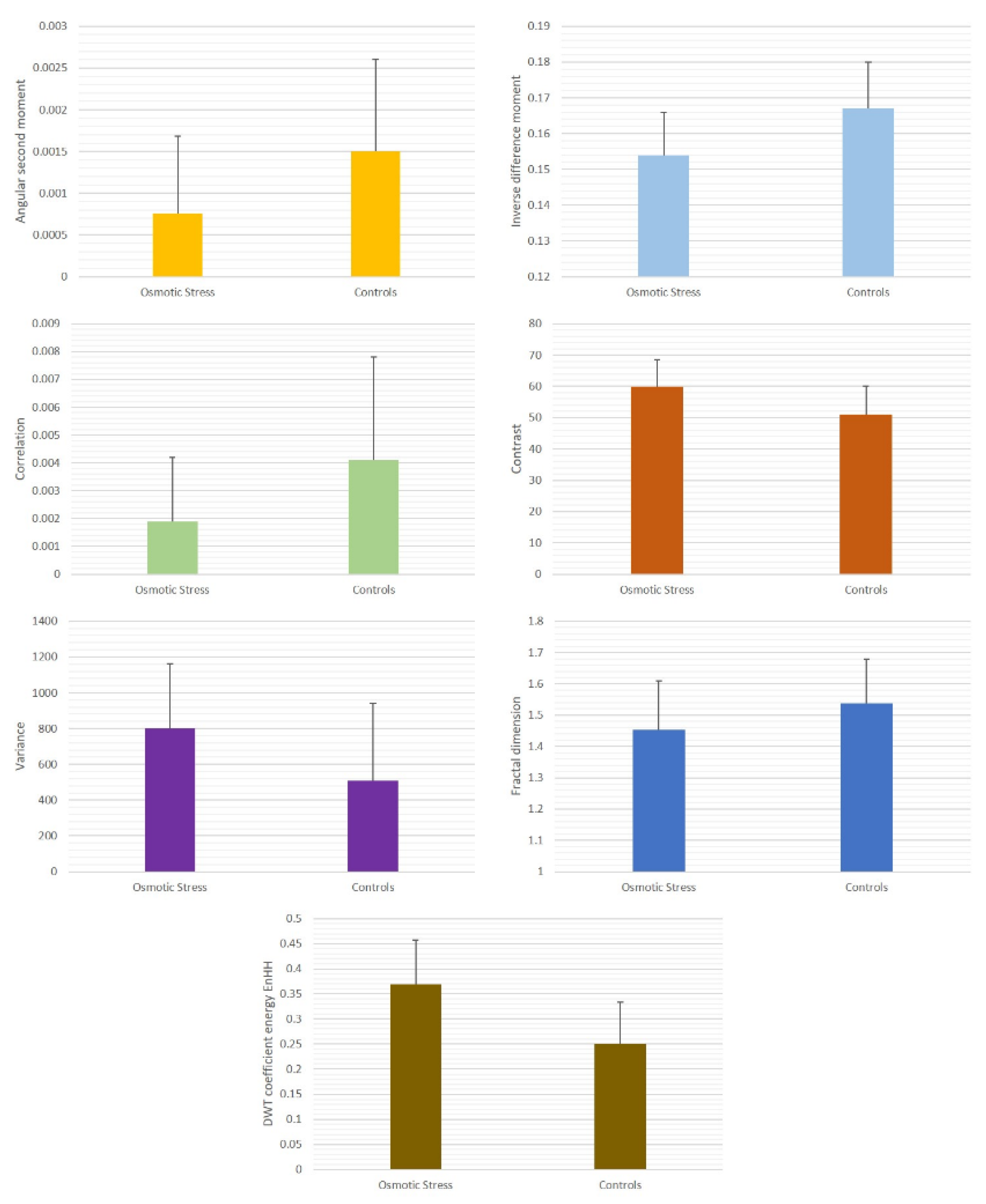
Figure 1). As in our previous work, for each ROI, the values of 5 GLCM indicators were determined: angular second moment (ASM), inverse difference moment (IDM), contrast (CON), correlation (COR), and textural variance (VAR). The standard GLCM method is performed on gray-scale images, where each pixel is given a value based on its gray intensity. After that, value pairs are analyzed using second-order statistics, and GLCM features are calculated.
Considering that
p(
i,
j) is the (
i,
j)th entry of the normalized co-occurrence matrix, the value of the inverse difference moment as the measure of local homogeneity was calculated as follows:
Angular second moment describing the uniformity (orderliness) within the distribution of gray levels was determined as follows:
Considering that μ and σ are the mean and the standard deviation, respectively, of rows x and y, within the normalized GLCM, the contrast and correlation features were determined as follows:
The contrast in these terms essentially relates to the degree of variation of gray level intensities in the two-dimensional signal, whereas the correlation represents the linear dependencies of gray levels on the other levels of the neighboring resolution units [
8,
28]. The level of dispersion of the gray level intensity distribution, when considering the value of the GLCM mean, was quantified as variance:
All the quantifications were analyzed as a part of a data frame (a two-dimensional data structure) in the Python Data Analysis Library (pandas)—an open-source platform for data analysis and manipulation.
Discrete wavelet transform (DWT) analysis of nuclear ROIs was performed in “Mazda” software previously prepared for the COST B21 European project “Physiological modelling of MR Image formation” and COST B11 AQ6 European project “Quantitative Analysis of Magnetic Resonance Image Texture”. The platform was created by Dr. Michal Strzelecki and Dr. Piotr Szczypinski (Institute of Electronics, Technical University of Lodz, Poland) and can perform a variety of tasks related to texture analysis [
29,
30,
31,
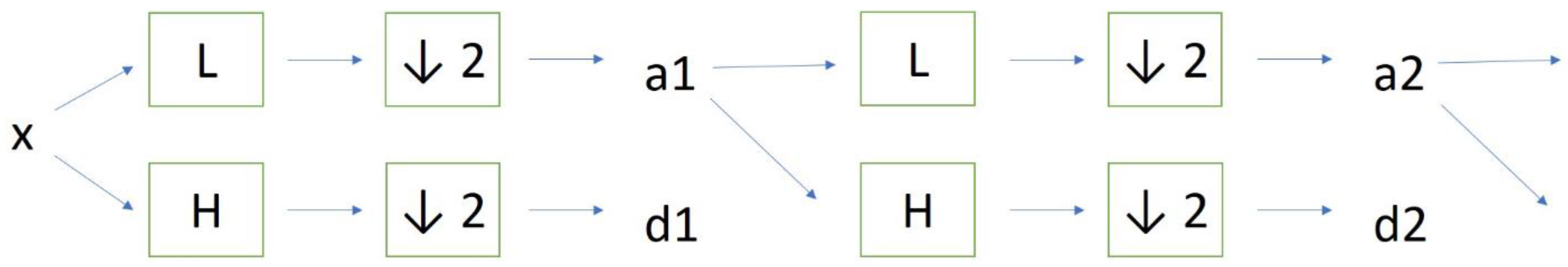
32]. For the purpose of our study, we calculated wavelet coefficient energy during a filtering cascade of rows and columns of data using high-pass filtering (
Figure 2). Briefly, the linear transformation was performed on data vectors which had the length of an integer power of two. The vectors were transformed to the same length but numerically different vectors, after which the data was separated into various frequency components depending on the scale. Factor 2 subsampling was performed after a cascade of filterings was implemented on the data. We used different combinations of low-pass (L) and high-pass filters (H). For the details on the procedure, the reader is referred to the previously published works on the method [
29,
33].
The energy (En) was calculated as follows:
where subband locations are marked as x and y, and n represents the number of ROI pixels.
Fractal analysis was carried out in FracLac, V. 2.5—a platform designed for ImageJ software by A. Karperien, Charles Sturt University, Australia/Canada—previously used on numerous occasions for description and quantification of complex biological structures and phenomena [
34,
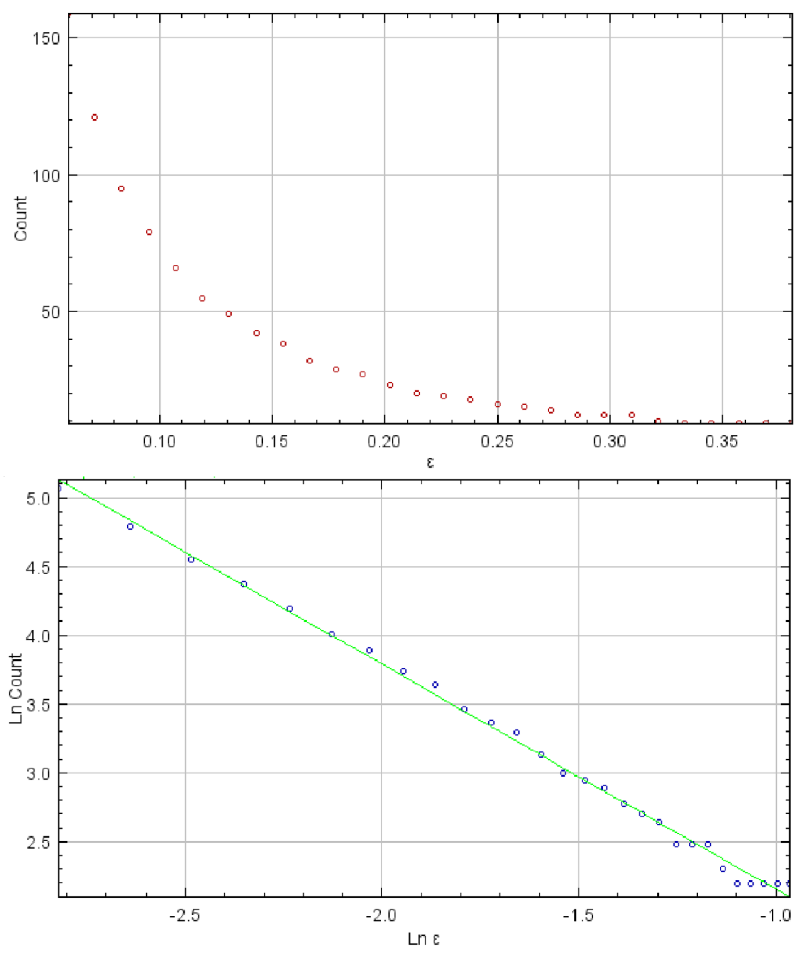
35]. For each ROI, after binarization, we calculated the value of the fractal dimension using the box-counting method. As explained in previous publications, this method applies a number of boxes over the structure at different scales (ε), after which a graph is created representing the logarithmic value of the number of boxes (N) at least partially filled with the structure (
Figure 3). The fractal dimension is calculated based on the slope of the linear regression of log(1/ε) versus log N(ε) for all ε [
20,
35]. Fractal dimension may be viewed as an indirect measure of complexity and level of detail and previously was used to detect small, microscopic alterations in biological structures that are generally not visible using conventional means.
Raw data obtained from fractal, GLCM, and DWT analyses were statistically analyzed in SPSS (v. 25.0, IBM Corporation, Chicago, IL, USA). The multivariate analysis of variance (MANOVA) was used to determine whether there were any differences between the two groups of cells. Regarding the ML models, the raw data were later used as inputs for training and testing ML models. The first model was based on a support vector machine algorithm, a supervised learning non-probabilistic binary linear classifier. This model regards individual data points as a mathematical p-dimensional vector, and its main task is developing the ability to separate the data along a (p-1)-dimensional hyperplane(s). Support vector machines are commonly used both for the classification and regression of data in biological sciences, with frequent application in image analysis and prediction of biological phenomena based on two-dimensional signals.
The second machine learning model involved the development of random decision forests classifier, an ensemble method in which multiple decision trees are constructed and averaged for their prediction output. Generally, random forests are more capable of classification compared to individual trees, although the interpretability of the model may be reduced in some circumstances. As with the support vector machine, random forests are a form of supervised learning, meaning that the model learns when given a series of examples with known input and output. During the training, the model reveals a pattern of data organization or a rule that connects inputs with output.
Both models were trained in scikit-learn machine learning library for the Python programming language using Google Colaboratory—a platform which enables the scientist to write and execute Python code in a browser. The Colaboratory includes a hosted Jupyter notebook service which can be used to import various libraries and modules for machine learning. The target data of both trained models were the class of the cell which was set to either ‘0’ for the controls or ‘1’ for the cells exposed to the hyperosmotic environment. Approximately 80% of the sample was used for training, and 20% was used for model testing. Classification accuracy for both models was quantified using the scikit-learn “metrics” module [
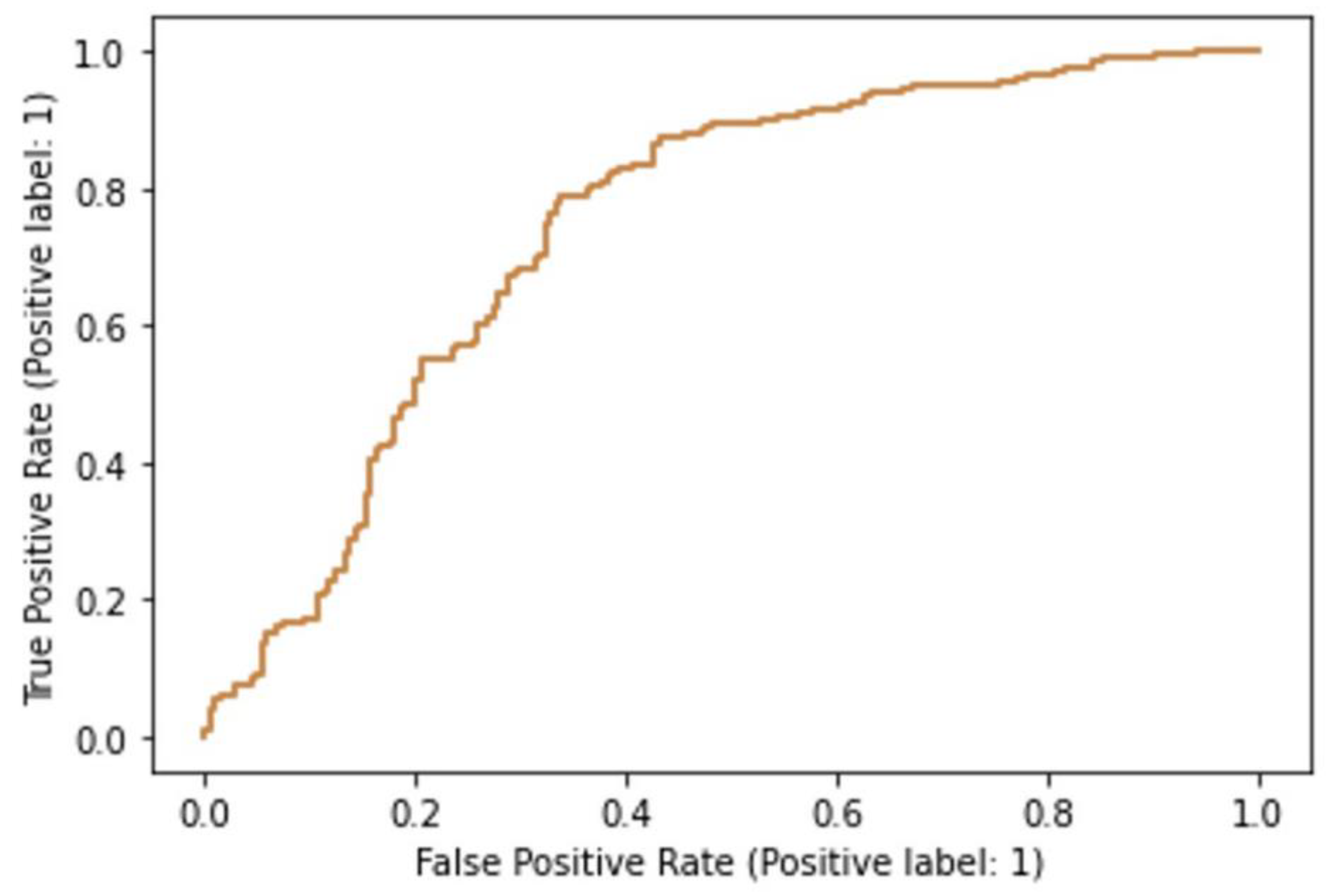
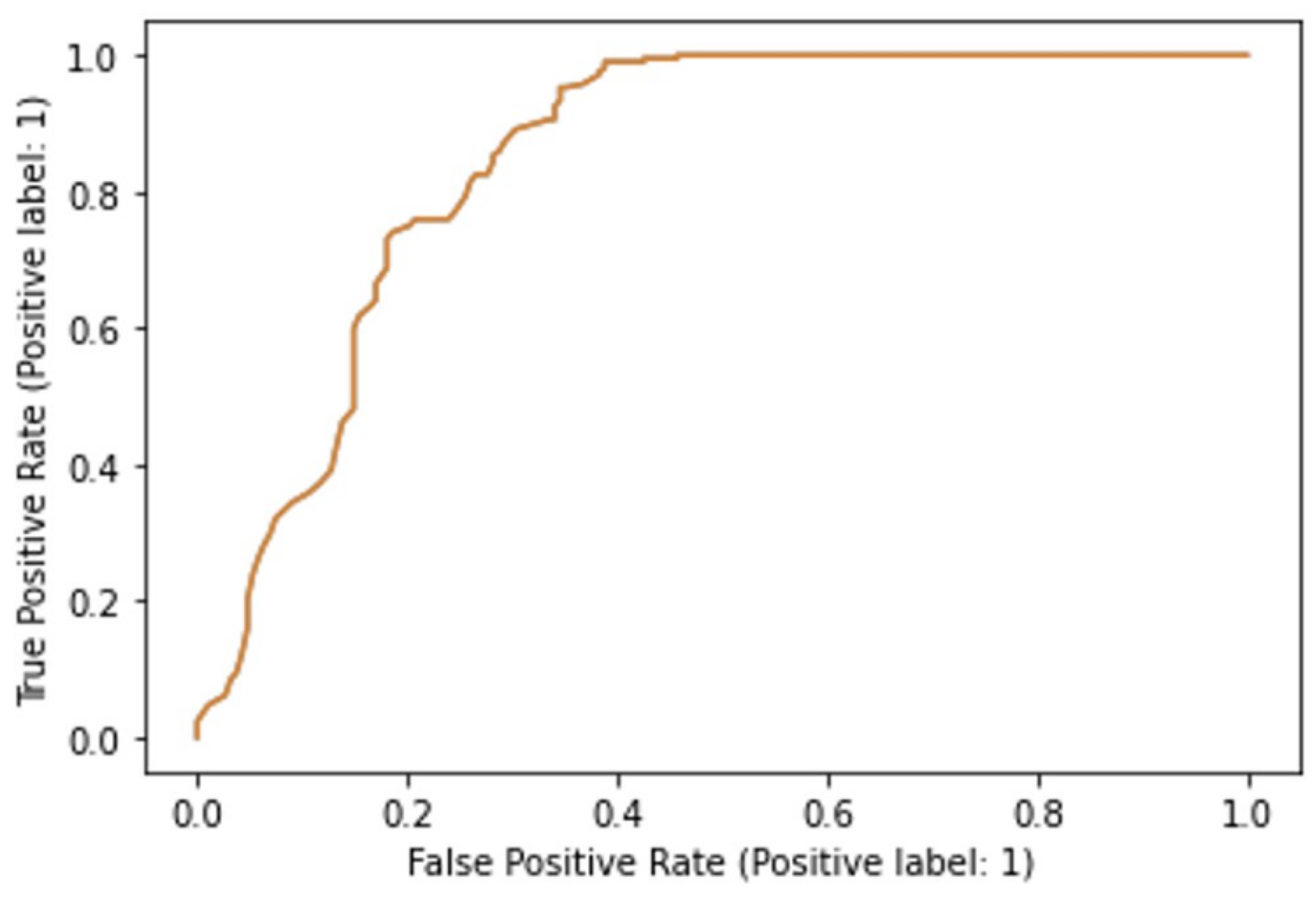
36]. Optimization of hyperparameters was performed with Grid Search (GridSearchCV module in scikit-learn). For the SVM classifier, it was determined that the optimal hyperparameters were radial basis function (RBF) kernel, “C” hyperparameter of 1, and “gamma” set to “scale”. For the random forests model, the “entropy” value was found to be the optimal “criterion” and “log 2” optimal for the maximal number of features. The optimal number of estimators was found to be 100. For the evaluation of the discriminatory power of the models, we used receiver operating characteristics (ROC) analysis, also in the scikit-learn “metrics” module, and the area under the ROC curve was determined. Furthermore, in scikit-learn, we calculated the classification accuracies of the models.
4. Discussion
Our study shows that exposing yeast cells to hyperosmotic stress results in significant changes in the nuclear texture, which can be quantified using GLCM and DWT methods, as well as significant changes in the nuclear fractal dimension. We also propose using GLCM, fractal, and DWT indicators as input data for machine learning models, such as support vector machines and random forests. The models trained on a relatively small sample achieved a decent level of classification accuracy and discriminatory power when distinguishing between treated and healthy cells. These findings and models can serve as a foundation for further developing AI-based methods for detecting osmotic shock injury in cells and their components.
In the field of cell biology, the use of computational methods, such as GLCM, DWT, and fractal analysis, to analyze the texture of cell nuclei is relatively new and has not been widely tested. There are several limitations and concerns regarding the sensitivity and validity of these methods. They can be applied to various cell populations, both in vivo and in vitro, and can provide information about structural homogeneity in cell and tissue micrographs [
17,
20,
35]. However, it should be noted that textural homogeneity does not always correlate with homogeneity in histological terms. The use of DWT indicators for quantifying textural heterogeneity also requires further validation by future studies. Likewise, fractal analysis is a mathematical and biophysical method that can be used to infer the complexity of a signal, whether one-dimensional or two-dimensional, as in our study, but its potential applications in this field also remain to be confirmed by future research.
This is not the first time we have used Saccharomyces cerevisiae to create machine learning models for assessing cell damage. In a recent study, we examined the impact of sublethal doses of ethanol on GLCM indicators such as angular second moment and inverse difference [
8]. Ethanol caused similar changes as hyperosmotic stress caused by NaCl, with a reduction in textural uniformity and local homogeneity of cell nuclei. In addition to GLCM analysis, we proposed machine learning models based on random trees, multilayer perceptron, and binomial logistic regression. All three models showed high classification accuracy, and the neural network performed best in terms of the area under the receiver operating characteristics curve (the AUC equaled 0.87). The changes in GLCM indicators are somewhat in accordance with the results of our current study since alcohol can cause hyperosmotic stress under certain conditions. However, we should note that these alterations in the nuclear structure are more likely to result from ethanol-induced damage to the genetic material of the cells or the reorganization of chromatin in nuclei due to the activation of specific signaling pathways associated with ethanol damage.
Fractal analysis has previously been used to indirectly quantify structural complexity and level of detail in micrographs of cells and tissues [
20,
21]. The analysis of neurons in the central and peripheral nervous system is perhaps the most extensive application of this method in microscopy, as fractal dimension can aid in the assessment of branching patterns of axons and dendrites. [
37,
38,
39]. However, there have been several studies that tried to quantify fractal dimension and other fractal indicators in cell nuclei and chromatin. The fractal dimension of euchromatin and heterochromatin seems to differ. In recent years, there have been attempts to introduce the so-called “fractal globule” model of chromatin organization as an alternative to the conventional equilibrium model. Chromatin, as a macromolecule, and DNA possess certain self-similarity traits, and their fractality remains to be fully investigated. In our study, we applied fractal analysis solely to identify subtle morphological alterations in cell nuclei and to generate data for the ML model training.
Exposure to a hyperosmotic environment in Saccharomyces cerevisiae yeast cells leads to a significant reduction of cell volume and activation of numerous adaptation mechanisms [
40,
41,
42]. These cells are exceptionally resilient to high tonicity; the viability is generally preserved, and the cells have numerous well-preserved genes that are involved in osmoprotection. Severe osmotic shock in yeast often leads to cell cycle arrest, growth inhibition, and reduced metabolic activity. Glycerol, trehalose, and erythritol as compatible solutes to NaCl are being produced to counteract the high osmolarity of the extracellular space. In addition, during hyperosmotic stress caused by NaCl or other osmotically active compounds, a number of stress-response pathways are activated, such as the high osmolarity glycerol (HOG) pathway or the stress-activated protein kinase pathway (SAPK). This all leads to significant changes in DNA transcription and gene expression and possibly to the reorganization of nuclear chromatin patterns. Furthermore, hyperosmotic stress may be associated with the increased production of reactive oxygen species and oxidative stress to the cell genetic material. While it is currently unclear which of these processes is responsible for the observed changes in computational texture indicators, it is plausible to speculate that the primary factor contributing to these changes is the epigenetic alterations that occur as part of the cell’s adaptation mechanisms to damage.
The most interesting aspect of our study is probably the fact that computational methods were able to detect subtle changes in cell morphology that were not clearly visible during standard microscopy. The analyzed cells did not show visible signs of programmed cell death, necrosis, or substantial nuclear injury. Even to the researcher with wide previous experience in the fields of microscopy and cell biology, cells from both groups appeared morphologically identical, and there was no subjective way of adequately separating and classifying them into the two groups. Some minor alterations in nuclear structure, such as the darkened areas on the nuclear periphery (visible in
Figure 1), were not specific to the experimental group and could easily be a physiological variation characteristic of this cell type or a minor variation in light exposure and white balance during microscopy and cell acquisition. On the other hand, computational methods showed significant differences in fractal, textural, and wavelet indicators between the groups. This potentially demonstrates the power of these methods in detecting discrete morphological phenomena, increasing their scientific value in the field of pathology. In the future, these methods may be useful as part of computer-aided diagnostic systems in pathology for classifying different types of pathological cells or separating pathologically changed cells from intact cells in various experimental and clinical conditions. However, the various steps and other limitations of these methods will need to be addressed before this can happen. There are a few significant limitations of our study that may hamper its impact in the fields of microscopy and cell biology. As mentioned earlier, all the applied computational methods are relatively new in this area of research. They have not undergone rigorous testing for their validity, accuracy, and quality assurance in general. Inter- and intra-observer reliability of the methods is undetermined for most cell populations and tissues. Despite some efforts in the past to perform quality assurance, this remains a significant obstacle to the use of the techniques in contemporary histology and pathology. The second limitation is the relatively high degree of variability of the values of fractal and GLCM indicators across different softer platforms and under different experimental settings. For example, the values of the angular second moment and inverse difference moment can drastically differ when micrographs are created in different sizes and resolutions or when a different image acquisition system is used. The same applies to various microscope settings such as exposure, hue, saturation, and white balance, which may greatly depend on the type of microscope, the imaging device and default preferences set within imaging software. Finally, the fact that we were able to observe changes in computational indications in this yeast culture does not necessarily imply that the changes are present in other cultures, particularly when various fixation and staining protocols are applied. To draw definitive conclusions on the changes in chromatin textural patterns during hyperosmotic stress and the potential usefulness of pattern recognition approaches in this field, future studies should utilize specific staining procedures aimed at visualizing chromatin structure in yeast. In our research, we only quantified 5 GLCM indicators: angular second moment, inverse difference moment, textural contrast, correlation, and variance. However, GLCM and other similar forms of textural analysis can be used to obtain many more textural features. The examples include entropy, sum entropy, difference entropy, information measures of correlation, maximal correlation coefficient and other quantifications. According to the original work of Haralick et al. [
43], a total of 28 textural features can be theoretically extracted from gray-tone spatial-dependence matrices, and today different computing platforms can be used to quantify the majority of them. Future studies would need to use all possible features to design the ML models with the best performance before this approach can be included in contemporary cell biology and pathology practice. The same reasoning applies to fractal analysis, where other features can also be quantified apart from the fractal dimension. The most important example would be the lacunarity feature, a measure of the level of “gappiness” within a fractal, which is frequently calculated alongside the fractal dimension to provide better insight into the changes in complexity. In the future, it would be interesting to see the classification accuracy and discriminatory power of the RF and SVM models constructed with the combination of lacunarity and GLCM data as inputs.
The machine learning approach applied in our study also has certain limitations that need to be discussed. Support vector machine and random forest are just two of many supervised ML algorithms that can be trained by presenting a series of examples of input and (correct) output or target data [
44]. Other models that are also potentially valuable include neural networks, various decision trees other than random forest, as well as models that rely on binomial logistic regression analysis. Some of these approaches may be better for the identification of specific patterns within the GLCM and DWT data and may yield higher discriminatory power and classification accuracy when trained in this setting. In the future, it would be advisable to develop and compare all possible ML models, after which the best one could be deployed as a web or other application. In our study, the samples used for training and testing were relatively low. It is possible that with a larger amount of especially GLCM data, one could develop a complex model (i.e., the one based on a multilayer perceptron network) that would have outstanding performance in cell classification. Finally, another important limitation concerning ML relates to the fact that ML models, in general, suffer from low interpretability. Random forest and support vector machines are no exception, and although we may obtain interesting results on their performance, it is still difficult to explain how the model actually functions and what actual inner mechanisms lead to its decisions in cell classification. This, along with the abovementioned general lack of quality assurance of computational techniques for data generation, greatly limits the overall reproducibility of the results. Future works will have to be focused on how to resolve these issues before these types of models become ready to be integrated into contemporary research and diagnostic protocols in pathology and other fields.


 ,
, 


