Cross-Correlation Multifractal Analysis of Technological Innovation, Financial Market and Real Economy Indices

Abstract

Technological innovation, the financial market, and the real economy are mutually promoting and restricting. Considering the interference of market-noise information, this paper applies the wavelet-denoising method of the soft- and hard-threshold compromise functions to process the original information so as to eliminate the noise information, and combines multifractal detrended cross-correlation analysis with the sliding-window approach, focusing on the change in the Hurst index and the parameter change in the multifractal spectrum to explore the interaction in between. The research results show that there is a certain cross-correlation among technological-innovation, financial-market, and real-economy indices. Firstly, the cross-correlation among them has significant multifractal characteristics rather than single-fractal characteristics. Secondly, the fractal characteristics reveal the long memory of the interaction among the three indices. Thirdly, there are also obvious differences in the degree of local chaos and volatility of the interaction. Fourthly, the cross-correlation among technological-innovation, financial-market, and real-economy indices has significant multifractal characteristics rather than single-fractal characteristics. In comparison, the cross-correlation multifractal characteristics among technological innovation, the financial market, and the real economy are time-varying, and the cross-correlation multifractal characteristics between the technological-innovation index and the real-economy index are the most obvious.

1. Introduction

The financial market and the real economy have a mutually reinforcing relationship. The financial market provides the required financial support for the actual economy’s development. The real economy serves as the tangible foundation for the growth of the financial market. Technological innovation empowers the traditional financial market and provides continuous vitality for the financial market’s transformation and upgrading, whereas the financial market plays an indispensable role in accelerating entrepreneurial investment, technology realization, and production promotion. Technological innovation has stimulated innovative financial products and services to provide more efficient and convenient financing channels for the development of the real economy, fueled by cutting-edge technologies such as big data, artificial intelligence, cloud computing, blockchain, and mobile internet [1]. Technological innovation has increased the availability of financial services, raised the efficiency of capital distribution in the real economy, and played a key role in fostering the development of the real economy. Excessive integration and expansion of the financial market and technological innovation, on the other hand, can easily cause an imbalance in the financial-industry structure, separate the development of financial innovation from the real economy, and produce a risk-spillover effect, leading to a gradual decline in the financial market’s and technological innovation’s ability to serve the real economy [2].

Modern financial theory has transformed the analysis of this problem from qualitative to quantitative and has also produced a large number of scientific-analysis methods, such as financial-market microstructure theory, behavioral-finance theory, and fractal-market theory, in terms of the interrelationship between technological-innovation, financial-market, and real-economy indices. Because financial data frequently exhibit peak and thick tail features, self-similarity, long memory, and volatility concentration, the fractal-market theory based on nonlinear dynamic systems can accurately reflect the real condition of the financial market. Furthermore, fractal-market theory deviates from the original linear research paradigm by describing the price-fluctuation characteristics of financial markets in greater depth and detail [3]. Among these, the multifractal theory can express precise information about financial-asset values at diverse time scales and degrees of volatility [4,5], better capturing the financial market’s complex nonlinear dynamic characteristics. Therefore, this research examines the relationship between technical-innovation, financial-market, and real-economy indices from a multifractal perspective.

2. Literature Review

The impact mechanism of technological innovation and the financial market on the development of the real economy is mainly manifested in that the financial market acts on technological innovation and the real economy from three aspects: provision of funds [6], innovation decentralization [7], and incentive supervision [8]. The financial market has gathered equity funds for technological innovation and provided financial support for the development of technological-innovation activities. Advanced technology promotes the development of the real economy and can effectively improve the innovation level and production efficiency of enterprises, make the industrial structure more reasonable, and then promote the development of the real economy. Technological innovation provides technical means for the development of financial markets, breaks through technical difficulties in financial markets, and enriches financial products. At the same time, the innovation-feedback effect brought by technological innovation also improves the financial system [9].

The interaction between technological innovation, the financial market, and the real economy has been a hot research topic in academic circles in recent years. Scholars have published papers about the impact of scientific and technological finance on economic development, and most of them believe that the use of industry-finance data or industry stock indices can roughly reflect the relevant performance between industries [10,11,12]. Dagar et al. constructed the technological-innovation-development index and used the GMM two-step test to draw the conclusion that technological innovation has a significant role in promoting the upgrading of industrial structure and can promote economic growth [13]. Qi and Li analyzed the stock-price data of listed companies in the manufacturing industry, summarized the dependency between the real economy and financial technology, and found that the various industries and technology companies in the real economy were greatly affected by the stock-price fluctuations of AI, blockchain, and large data-technology companies in financial technology, showing a positive correlation [14]. Peng and Ke employed the R-vine Copula approach to successfully examine the risk-spillover impact between financial technology and the real economy [15]. They chose stock-index samples to fit the residual tail features of the time series. Furthermore, some scholars use industry data to research and discover that there is a threshold effect in Fintech, which can support real-economy growth in the early stages of Fintech development and restrict real-economy growth in the later stages [16]. Some studies suggest that Fintech can improve the optimization and upgrading of industrial structure through basic technology innovation and development, hence encouraging economic growth [17]. The rise of financial technology has resulted in the pursuit of capital, with capital flowing to artificial intelligence, blockchain, and other underlying technologies, in combination with the industrial linkage effect, to drive the upgrading of industrial structure and thus promote high-quality economic development [18].

The concept of the fractal was first proposed by Mandelbrot, and the definition emphasizes the similarity between the whole and the part of the fractal [19]. Peters put forward the fractal-market hypothesis based on the fractal theory proposed by Mandelbrot. It is based on the nonlinear paradigm and believes that the capital market is a complex nonlinear dynamic system with the characteristics of interactivity and adaptability [20]. The market’s information flow is frequently unstable, difficult to conform to conventional modeling assumptions, and frequently volatile. In contrast, the fractal statistical-analysis approach based on fractal and chaos theory can effectively explain the nonlinear fundamental features of the market. This makes it difficult for some standard statistical-analysis methods to characterize the volatility characteristics of the market.

Fractal-theory research techniques have seen constant innovation and development in recent years. The rescaled range analysis (R/S), put forth by the hydrologist Hurst, is particularly well liked in early fractal research [21]. Previous studies have confirmed that there is long-term autocorrelation in the capital market, which means that the capital market is not an efficient market [22,23]. However, the R/S analysis method is relatively sensitive to outliers and dependent on extreme values, so it is mostly used to analyze non-trending stationary time series, whereas the analysis of non-stationary time series is prone to errors. In order to study the non-stationary time series with trends, Peng et al. proposed the DFA analysis method [24]. This method introduces a long-term power–law relationship in time-series analysis to supplement short-term correlation conditions to avoid the occurrence of false correlation. The Hurst result calculated by the DFA method is more accurate than that estimated by the R/S analysis method. Subsequently, scholars introduced a multifractal on the basis of the DFA method and evolved it into a more applicable MF-DFA analysis method [25]. Gulich and Zunino conducted a comprehensive and systematic analysis of the algorithm to determine the parameters in the MF-DFA method and studied the natural time series to ensure the effectiveness of the algorithm [26]. Unfortunately, this method can only study the long-term correlation of a single time series. In view of this, the DFA method has been expanded into a DCCA method that can explore the cross-correlation between two non-stationary time series [27]. As a result, the DCCA approach has been steadily used to develop the MF-DCCA approach, which can accurately and quantitatively examine the multifractal properties of two cross-correlation time series [28]. This method can be used in the capital market to examine the cross-correlation [29].

The processing of economic or financial time series is the key to empirical analysis. If a large amount of noise data is directly used, it is very likely to bias the research results. The existing research results show that using special methods to denoise the time series can reduce the instability of the time series to a certain extent and ensure that the research results are more authentic and reliable [30]. In the early days, the moving average was one of the most widely used denoising methods. Although this method is simple, it is easy to remove much useful information when denoising [31]. The Fourier-transform filtering method is another traditional denoising method, but it can only be processed in the whole time domain and cannot give the change of the signal at the specific node. A small mutation of the signal is likely to affect the whole analysis result [32]. The wavelet-transform method is a relatively effective time-frequency denoising-analysis method that can overcome the shortcomings of the Fourier-transform method [33]. Common wavelet-denoising methods mainly include modulus maximum-reconstruction denoising and threshold denoising. Mallat proposed a denoising method based on modulus maxima. Its idea is to remove the amplitude extreme points that decrease with the increase in scale by observing the change rule of the modulus maxima of the wavelet transform at different scales and only retain the amplitude points that increase with the increase in scale so as to achieve the denoising effect [34]. This method is more suitable for the situation that the signal contains white noise and has many singular points and can effectively retain the information of singular points. The wavelet threshold denoising algorithm proposed by Donoho and Johnstone has been widely used because of its simple operation logic and good denoising effect [35]. In the wavelet-threshold denoising method, the selection of threshold function is also very important. The previously widely used hard-threshold function and soft-threshold function have some defects [36]. For example, the hard-threshold function preserves the points whose absolute value is greater than the threshold value and zeros the points whose absolute value is less than the threshold value. This processing causes sudden changes in the wavelet domain, resulting in local jitter of the results after denoising and discontinuity of the results. The defect of the soft-threshold function is that the derivative is discontinuous, and there is a constant deviation between the estimated wavelet coefficients and the wavelet coefficients of the processed signal. In addition, most de-noising processing has been successfully applied to various disciplines such as signal analysis, image processing, and seismic survey. The application of time series in the financial market or economic market is still in the exploration stage, but it can be expected that wavelet denoising has certain advantages in processing time-series data.

To sum up, the existing research on the interaction between scientific and technological innovation, the financial market, and the real economy is mainly focused on their impact, but few explore the multifractal characteristics between them from the perspective of cross-correlation. Moreover, most of the research is based on linear methods, and the sample data selected are based on the direct data of the market, ignoring the impact of noise information. Therefore, this paper firstly uses the wavelet-threshold denoising method to eliminate the noise impact in scientific- and technological-innovation, financial-market and real-economy indices; retain effective fluctuation information; and use the sliding-window segmentation method (SW) to optimize. Then, with the help of the MF-DCCA method in the nonlinear field, the cross-correlation fractal features are studied in terms of fractal multiplicity, long-term memory, similarity, and singularity of the fractal spectrum to better reveal the complex relationship.

3. Method

3.1. Wavelet-Threshold Denoising Method

The basic principle of wavelet-threshold denoising is to set a threshold to process high-frequency noise signals. Specifically, useful signals with wavelet coefficients greater than the threshold are shrunk and retained. The noise of the wavelet coefficient lower than the threshold value is eliminated. The one-dimensional signal model with noise can be expressed as [37]:

$$f\left(t\right)=s\left(t\right)+n\left(t\right)$$

(1)

where $f\left(t\right)$ is the signal with noise, $s\left(t\right)$ is the effective signal in the original signal, $n\left(t\right)$ is the noise signal, and $t$ is the time variable.

Specifically, the denoising process of wavelet-threshold denoising can be divided into three steps. Firstly, the signal containing noise is decomposed by a wavelet. The appropriate wavelet-basis function and decomposition scale for wavelet decomposition is selected to obtain a set of wavelet coefficients. Secondly, the high-frequency coefficients of each layer of wavelet decomposition are processed by threshold quantization to obtain the estimated value of wavelet coefficients. Finally, the wavelet coefficients processed by threshold quantization are transformed by an inverse wavelet to reconstruct the signal and obtain the denoised signal.

The proper threshold function will affect the denoising effect. When the signal is decomposed, the wavelet coefficients need to be threshold processed. The commonly used threshold functions are divided into hard-threshold function and soft-threshold function [38]. The mathematical expression of the hard-threshold function is as follows:

$${\widehat{\omega }}_{j,k}=\{\begin{array}{c}{\omega }_{j,k} \left|{\omega }_{j,k}\right|\ge \lambda \\ 0 \left|{\omega }_{j,k}\right|<\lambda \end{array}$$

(2)

where $\lambda$ represents the threshold value, the estimated value of the wavelet coefficients is expressed by ${\widehat{\omega }}_{j,k}$, and the wavelet coefficient of the $j$-th layer is represented by ${\omega }_{j,k}$.

The mathematical expression of the soft-threshold function is as follows:

$${\widehat{\omega }}_{j,k}=\{\begin{array}{c}sign\left({\omega }_{j,k}\right)\left(\left|{\omega }_{j,k}\right|-\lambda \right) \left|{\omega }_{j,k}\right|\ge \lambda \\ 0 \left|{\omega }_{j,k}\right|<\lambda \end{array}$$

(3)

However, the above threshold functions have certain limitations in practical applications. Therefore, the soft- and hard-threshold compromise function can be introduced to overcome the discontinuity problem in the hard-threshold function and reduce the constant deviation in the soft-threshold function. The expression is as follows:

$${\widehat{\omega }}_{j,k}=\{\begin{array}{c}\left(1-\mu \right){\omega }_{j,k}+\mu sign\left({\omega }_{j,k}\right)\left(\left|{\omega }_{j,k}\right|-\lambda \right) \left|{\omega }_{j,k}\right|\ge \lambda \\ 0 \left|{\omega }_{j,k}\right|<\lambda \end{array}$$

(4)

where $\mu$ is the weighting factor, and is usually set to 0.5.

$$\lambda =\sigma \sqrt{2lnN}$$

(5)

$$\sigma =\frac{{{\displaystyle \sum }}_{k=1}^n\left|{\widehat{\omega }}_{j,k}\right|}{0.6475n}$$

(6)

where $\sigma$ is the mean square error of the $j$-th layer wavelet transform.

In the process of denoising, the selection of wavelet function is also very important. At present, there are dozens of wavelet functions that have been developed and applied. These wavelet functions are suitable for different situations due to their own characteristics. The most widely applied are Daubechies wavelet-basis function (dbN), Coiflet wavelet-basis function (coifN), and Symlets wavelet-basis function (symN). Different wavelet bases have different degrees of orthogonality, compact support, vanishing moment, and symmetry [39]. After the wavelet function with orthogonality is transformed, the correlation between wavelet coefficients will not be destroyed by the transformation, so it has high noise-reduction ability. The wavelet-basis function with compact support has better local noise resolution and denoising ability when the support width is small. The vanishing moment can smooth the high-order part of signals when analyzing and processing the time-series data with strong fluctuations. The symmetric-wavelet function can reduce the distortion of signal reconstruction to some extent. In addition, it is necessary to consider the appropriate number of decomposition layers in wavelet denoising.

3.2. Multifractal Detrended Cross-Correlation-Analysis Method

3.2.1. The DCCA Method

In order to study the cross-correlation between two variable sequences, detrended cross-correlation analysis (DCCA) can be used [27]. This method is based on the detrended covariance-analysis method, which can filter out the trend components of each order to eliminate non-stationary influence in the original sequence.

Suppose there are two time series $\left\{x\left(t\right)\right\}$ and $\left\{y\left(t\right)\right\}$ of length $N, t=1,2,\cdots ,N$. The cumulative deviation series of the two original time series can be calculated by the following formulas:

$$X\left(t\right)={\displaystyle \sum }_{k=1}^t\left(x\left(k\right)-\overline{x}\right), t=1,2,\cdots ,N$$

(7)

$$Y\left(t\right)={\displaystyle \sum }_{k=1}^t\left(y\left(k\right)-\overline{y}\right), t=1,2,\cdots ,N$$

(8)

where $\overline{x}$ and $\overline{y}$ are the mean of the sequence, $\overline{x}=\frac{1}{N}{\displaystyle \sum }_{t=1}^{N}x\left(t\right)$, $\overline{y}=\frac{1}{N}{\displaystyle \sum }_{t=1}^{N}y\left(t\right)$.

The cumulative-deviation sequence is divided into equal-length subsequences. The least-square fitting is performed for each subsequence, and the fitting curves ${\tilde{X}}_v\left(i\right)$ and ${\tilde{Y}}_v\left(i\right)$ are obtained. Then, each subsequence is detrended, and the covariance function of the detrended subsequence is finally obtained.

For $v=1,2,\cdots ,N_s$, the local covariance function is:

$$F^2\left(s,v\right)=\frac{1}{s}{\displaystyle \sum }_{i=1}^s\left\{X\left[\left(v-1\right)s+i\right]-{\tilde{X}}_v\left(i\right)\right\}\times \left\{Y\left[\left(v-1\right)s+i\right]-{\tilde{Y}}_v\left(i\right)\right\}$$

(9)

For $v=N_s+1,\cdots , 2N_s$, the following formula is established:

$$F^2\left(s,v\right)=\frac{1}{s}{\displaystyle \sum }_{i=1}^s\left\{X\left[N-\left(v-N_s\right)s+i\right]-{\tilde{X}}_v\left(i\right)\right\}\times \left\{Y\left[N-\left(v-N_s\right)s+i\right]-{\tilde{Y}}_v\left(i\right)\right\}$$

(10)

where the preceding $N_s$ subintervals represent the positive segmentation subsequence of the deviation sequence, and the following $N_s$ subintervals represent the segmentation subsequence after the reversal of the deviation sequence.

The mean value of the local covariance function of all subintervals is determined to obtain the fluctuation function described in the following formula:

$$F_q\left(s\right)=\frac{1}{2N_s}{\displaystyle \sum }_{v=1}^{2N_s}{F}^2\left(s,v\right)$$

(11)

The calculation can be repeated to obtain the fluctuation function under different scales $s$. The limitation of the DCCA method is that it can only reveal the single-fractal characteristics of mutual correlation. However, the existence of multifractal characteristics has gradually become a consensus in the academic community. Therefore, it is not comprehensive to focus solely on the single-fractal characteristics.

3.2.2. The MF-DCCA Method

The modeling process of the MF-DCCA method and the DCCA method is similar, and the detrended covariance function of the subsequence is described in the same way. The difference between the two methods is that the MF-DCCA method takes into account the different fluctuation order $q$ when calculating the fluctuation function, whereas the DCCA method only considers the single fluctuation order when calculating the fluctuation function [28].

The MF-DCCA method takes the mean of the local covariance of all subintervals, and the $q$-order fluctuation function can be obtained:

$$F_q\left(s\right)={\left\{\frac{1}{2N_s}{\displaystyle \sum }_{v=1}^{2N_s}{\left[F^2\left(s,v\right)\right]}^{q/2}\right\}}^{1/q}$$

(12)

In general, $q$ can be any real number that is non-zero. When the value of $q$ is 0, the following formula can be obtained from L’Hospital’s rule:

$$F_0\left(s\right)=exp\left\{\frac{1}{4N_s}{\displaystyle \sum }_{v=1}^{2N_s}\left[F^2\left(s,v\right)\right]\right\}$$

(13)

Then, the fluctuation function $F_q\left(s\right)$ corresponding to different scales $s$ is calculated. If there is a long-range power-law cross-correlation between the two time series, then the fluctuation function $F_q\left(s\right)$ and the time scale $s$ have the following relationship:

$$F_q\left(s\right)~s^{H_{xy}\left(q\right)}$$

(14)

Then, the following formula is established:

$$\mathit{log}{F}_q\left(s\right)=H_{xy}\left(q\right)\mathit{log}s+\mathit{log}A$$

(15)

For each $q$ value, the linear slope obtained by $\mathit{log}{F}_q\left(s\right)$ and $\mathit{log}s$ regression is $H_{xy}\left(q\right)$, which is called the generalized Hurst index. Whether $H_{xy}\left(q\right)$ changes with the change of fluctuation order $q$ can be used to describe whether the cross-correlation fractal characteristic between two variables is multiplicity. The value of $H_{xy}\left(q\right)$ can reflect whether the interaction between variables has the characteristics of long memory. For the larger fluctuation order $q$, $H_{xy}\left(q\right)$ transmits the scaling behavior that the larger fluctuation dominates. On the contrary, for negative or small fluctuation order $q$, $H_{xy}\left(q\right)$ transmits the scaling behavior that small fluctuation dominates. It is worth mentioning that when $q$ is 2, $H_{xy}\left(2\right)$ is the classical Hurst index.

The relation between the generalized Hurst index $H_{xy}\left(q\right)$ and the multifractal scale index $\tau \left(q\right)$ obtained by the MF-DCCA method is as follows:

$$\tau \left(q\right)=q{H}_{xy}\left(q\right)-1$$

(16)

If $\tau \left(q\right)$ and $q$ are linear, then the two time series have the characteristics of a single fractal. Otherwise, they present the characteristics of a multifractal. Through Legendre transformation, a singular exponent and multifractal spectrum can be obtained.

$$\alpha =H_{xy}\left(q\right)+q{H}_{xy}^{\prime }\left(q\right)$$

(17)

$$f\left(\alpha \right)=q\left[\alpha -H_{xy}\left(q\right)\right]+1$$

(18)

Among them, $\alpha$ is the singular index, which is used to describe the degree of singularity of sequence. $f\left(\alpha \right)$ is the multifractal spectrum whose value reflects the fractal dimension with singular index $\alpha$. The multifractal spectrum transmits a lot of valuable fluctuation information. For example, the multifractal intensity can be measured by the width of the fractal spectrum. The wider the fractal spectrum, the stronger the multifractal intensity of the correlation between variables.

3.2.3. The Improved MF-DCCA Based on the OSW Method

The traditional MF-DCCA method will inevitably produce fluctuation errors in the fitting process due to the discontinuity when the cumulative deviation sequence is divided into subintervals, which may lead to a decline in the accuracy of the scale-index estimation. In order to minimize the negative impact of data-point discontinuity, it has been considered that the sliding-window approach can further reduce the generation of fluctuation error [40]. The specific steps of splitting the deviation sequence into subintervals are described below.

The deviation sequence of each original signal can be regarded as consisting of $N_s$ non-overlapping equal sequences, namely, $N_s=int\left(N/s\right)$, and the length of the subsequences is $s$. In most cases, the length $N$ of the deviation sequence of each original signal is not divisible by the length $s$ of the subsequence. In order to make full use of all the data information, the data sequence is usually recalculated in the reverse direction, so $2N_s$ subintervals can be obtained.

In this study, the deviation sequence was divided into subintervals and the continuous overlapping-sliding-window (OSW) segmentation method was adopted to replace the original segmentation method. The idea of OSW is to set a fixed window length $s$, and then slide back in steps of unit length until the window reaches the end of the time series. The specific details are shown in Figure 1 below. In this way, the sequence information is continuous and none of redundant information is left.

The subsequence was divided by the continuous overlapping-sliding-window technique and the fluctuation analysis was carried out by the MF-DCCA method. The combination of these two can be called OSW-MF-DCCA, which reveals that the fractal discovery had certain robustness.

4. Empirical Analysis

4.1. Index Construction and Sample Selection

This study screened and weighted the data of different sectors in the stock market to construct comprehensive indices that can represent technological innovation, financial development, and the real economy. The main reason for starting from the original data in the stock market is that, first, the stock market is more sensitive to the perception of information, and fluctuations in any industry can be quickly reflected in the stock market. Second, stock-market data have the advantages of high integrity, strong continuity, and high frequency, whereas traditional economic data are often difficult to count. Therefore, the composite index constructed in the form of weighted stock data can largely reflect the actual situation of the industry.

This paper mainly selected and constructed the technological-innovation index (TI), financial-market index (FI), and real-economy index (RE) in the stock market to represent the overall situation of the technological-innovation industry, the financial industry, and the real-economy industry. In the actual selection of exponents, the TI selected the representative technology 100 index, which is mainly used to reflect the overall trend of company stocks with high-tech or independent innovation characteristics and has strong representation for the technology-innovation industry. The compilation of the FI and the RE refers to the compilation methods of S&P500 and CSI (China Securities Industry Index). The financial industry can be divided into the banking industry and the non-banking financial industry according to the classification basis of the Shenwan primary industry index. The FI was constructed by weighting the constituent stocks of the banking and non-banking financial industries. The RE is represented by the nine China securities-industry indices, which basically cover real-economy fields such as energy, information industry, industrial manufacturing, medical treatment, consumer goods, and agricultural products. Specifically, they are China Securities Energy, China Securities Material, China Securities Consumption, China Securities Optional Consumption, China Securities Information, China Securities Medicine, China Securities Telecom, China Securities Public Utility, and China Securities Industry. Through the weighted average of the constituent stocks of the real-economy industries, the RE was constructed. The data selected in this paper were daily data from January 2012 to December 2021, and the data were processed by logarithmic difference to improve the stability of the time series.

4.2. Descriptive Statistical Analysis

This study plotted the index time-series diagram of fluctuations of the TI, FI, and RE, as shown in Figure 2. In the figure, the horizontal axis represents the beginning of 2012 to the ending of 2021, and the vertical axis represents the fluctuation range of the data. The part above 0 represents the positive fluctuations, whereas the part below 0 represents the negative fluctuations caused by the adverse impact. It was found that the fluctuations of the TI, FI, and RE were more volatile, and their peaks were mainly concentrated during the stock-market crash in 2015 and the COVID-19 pandemic that started in 2019. It is worth noting that there were more obvious volatility aggregations during the two crises, which may have been caused by short-term noise interference, so the TI, FI, and RE were affected in a sustained way.

The descriptive statistics of the indices for the fundamental characteristics are listed in

Table 1. Descriptive statistical results.

Variable	Median	Mean	Std. Dev.	Skewness	Kurtosis	Jarque–Bera
TI	0.052	0.092	1.865	−0.622	5.850	979.535 *
FI	0.029	−0.047	1.459	−0.132	9.663	4504.348 *
RE	0.046	0.099	1.469	−0.943	9.145	4184.668 *

Note: * is significant at the confidence level of 1%.

.

It was found that skewness values of the TI, FI, and RE were less than 0, kurtosis values were greater than 3, and JB statistical values were far greater than the critical value of 9.210 based on observing Table 1. The distribution of indices presented the characteristics of peak and thick tails and non-normality, and fractal distribution better described the distribution of the indices. In addition, the median and mean of the TI, FI, and RE were all close to 0, which indicates that there were some extreme values in the three indices but that they still showed the characteristics of fluctuating around zero. The standard deviation of the TI was larger than that of the RE and FI, indicating that the TI had stronger volatility, possibly because the TI was more affected by noise.

In summary, the fluctuation-sequence charts and descriptive statistical results of the TI, FI, and RE show that the fluctuations of the TI, FI, and RE were relatively unstable. Large fluctuations were often accompanied by larger fluctuations, whereas small fluctuations were often accompanied by smaller fluctuations, presenting a relatively obvious volatility aggregation, which may have been due to the interference of noise information. If the study directly analyzes the original sequences and ignores the impact of exponential fluctuations, it may lead to a deviation in the research result. Therefore, in order to accurately analyze the fractal characteristics between the indices, it is necessary to first decrease the noise information.

4.3. Denoising Analysis

The time-series data in the financial market and economic market often have nonlinear characteristics, which may easily lead to the removal of much useful information in the process of denoising by traditional methods. Therefore, this paper used the wavelet-threshold denoising method by selecting different wavelet functions, decomposition layers, and threshold functions to denoise the indices according to the characteristics of the time series.

In the practical operation of wavelet-threshold denoising, the selection of threshold function is essential. This paper selected the $symN$ wavelet-basis function, which can deal with discrete wavelet transformation and has orthogonality and compact support. Although $symN$ and $dbN$ wavelet-basis function are similar in terms of support length, continuity, and filter length, $symN$ has better symmetry—that is, to a certain extent, it can reduce the phase distortion during signal analysis and reconstruction. Generally speaking, an appropriate vanishing moment is crucial in the analysis of financial or economic time series, and the mutability of time series makes it necessary to smooth the higher-order part of the signal. After repeated experiments to compare the denoising effect, the $sym6$ wavelet-basis function was selected in this paper.

At the same time, in the wavelet-threshold denoising, it is also very important to choose the appropriate number of decomposition layers. When the number of decomposition layers is higher, the more real signals will be removed from the signals in the denoising process. Therefore, in the actual operation of wavelet-threshold denoising, this paper selected one-layer denoising, which can not only effectively remove the noise information but also retain more useful information. More importantly, this paper applied the soft- and hard-threshold compromise function. It not only overcomes the discontinuity problem in the hard-threshold function but also reduces the constant deviation in the soft-threshold function.

The denoising signals of TI, FI, and RE based on the selected wavelet function, the number of decomposition layers, and the threshold function are shown in Figure 3.

In Figure 3, the fluctuation-aggregation degree of the denoising indices was weakened and the indices showed a certain stability. The original signals of the TI, FI, and RE fluctuated sharply during the stock-market crash in 2015 and the COVID-19 pandemic that started in 2019, and there were a lot of effective signals as well as noises. After using the wavelet-threshold denoising method, the fluctuation amplitude of signals decreased. In particular, the fluctuations of the indices during the crisis periods were still more volatile than that in the stable periods, which is consistent with the crisis circumstance at that time.

4.4. Fractal-Characteristics Analysis of Interaction Relationship

The improved OSW-MF-DCCA method in this paper can further avoid the pseudo-fluctuation errors to improve the accuracy of the results. Based on this, this paper focused on the TI, FI, and RE after wavelet-threshold denoising and quantitatively estimated their nonlinear cross-correlation relationship and multifractal characteristics via the MF-DCCA method. Referring to previous studies of scholars [41], the fluctuation order $q$ in this paper was set in the range of [−10, 10] for practical applications. In addition, Peng and other scholars pointed out that $5\le s\le N/4$ is more appropriate in practical applications [24], and this study referred to their recommended parameter-setting standard. In the calculation process, the fitting order of this study was set as the first order.

4.4.1. Multifractal Analysis

Fractal theory shows that the relationship between the Hurst value of the interaction between variables and the fluctuation order $q$ can effectively determine whether the fractal characteristic is single or multiple. If the Hurst index of the interaction between the two variables changes significantly with the change in the fluctuation order $q$, it means that the fractal characteristic of the interaction between the two variables is multiple. Otherwise, the interaction between the two is simplex.

In order to observe the interaction among the TI, FI, and RE in a more comprehensive way, this paper traversed all fluctuation orders. Figure 4 plots the relationship between the generalized Hurst value of cross-correlation and the fluctuation order $q$. For the purpose of comparison, the results of the TI and RE, the FI and RE, and the TI and FI were all plotted in the same chart, which can be seen in Figure 4a.

It is also worthwhile to pay attention to whether the fractal characteristics change with time changes. This paper analyzed the time variance of fractal characteristics, specifically observing the cross-correlation fractal characteristics in different periods and exploring the dynamic evolution of cross-correlation fractal characteristics from a local perspective. Firstly, the index data were divided into 10 sub-samples, and then the MF-DCCA method with sliding window was applied to each sub-sample to explore the cross-correlation fractal characteristics. The results are shown in Figure 4b–d. More sample data sets will be more persuasive to explain the research results.

In the case of the total sample, Figure 4a shows the $q$-$H\left(q\right)$ results of the cross-correlation among the TI, FI, and RE. The Hurst value of cross-correlation changed with the volatility order $q$. This indicates that the cross-correlation presented multifractal characteristics rather than single-fractal characteristics. Specifically, with the increase in the fluctuation order $q$, the Hurst value of cross-correlation among the TI, FI, and RE monotonically decreased. In contrast, with the change in the fluctuation order $q$, the Hurst value of the interaction between the RE and FI was roughly the same as the Hurst value of the interaction between the FI and TI, and the change range in the Hurst value was almost the same. However, the Hurst value of the interaction between the TI and RE underwent a bigger change. This shows that the multifractal characteristics of the interaction between TI and RE were more significant than those of other two. Such results also imply that the interaction between the TI and RE was relatively unstable.

In the sub-sample, Figure 4b–d clearly shows the dynamic evolution of the Hurst value of the interaction among the TI, FI, and RE in different periods. For the RE and TI, the Hurst value of cross-correlation between them decreased with an increase in the fluctuation order $q$ in any period. This shows that the cross-correlation fractal characteristic between the RE and TI was multiple at any time. For the FI and the RE, the Hurst value of cross-correlation between them in different periods was also not constant, which also means that they presented significant cross-correlation multifractal characteristics. The same performance happened in the cross-correlation fractal characteristics between FI and TI.

4.4.2. Time-Varying Memory Analysis

Studies related to complex dynamics suggest that whether the sequence is autocorrelation or cross-correlation, there may be a long-memory phenomenon in the process of fluctuations, which can also be called persistence. Simply put, it is about how long the impact of past information on the future will last, which can generally be measured by the value of the Hurst index.

In order to better understand the long-term-memory phenomenon of the interaction among the TI, FI, and RE, this paper observed the Hurst values of cross-correlation among the three indices in different periods and different degrees of volatility. Specifically, this study separately calculated the mean values of the Hurst indices of the interaction among TI, FI, and RE with the cases of when the fluctuation order $q$ was greater than 0 and when the fluctuation order $q$ was less than 0. The specific results are shown in Figure 5.

Figure 5 shows the Hurst values of cross-correlation among the TI, FI, and RE under different fluctuation degrees. Firstly, the mean values of the Hurst indices among the three indices were significantly higher than 0.5 when the fluctuation order $q$ was considered in all cases, which indicates that the interaction among the three indices was characterized by long memory in the overall situation. Secondly, when the volatility order $q$ was less than 0, the mean values of Hurst indices of cross-correlation among the three indices were also significantly higher than 0.5 under the fractal characteristics of small fluctuations. Moreover, the range of Hurst values above 0.5 in the case of small fluctuations was much larger than that of Hurst values above 0.5 in the overall case, which means that the interaction between the three indices in the period of small fluctuations had stronger long-term memory. Thirdly, when the fluctuation order $q$ was greater than 0, that is, in the case of large-fluctuation fractal characteristics, the mean values of the Hurst indices among the three indices were significantly lower than 0.5. This indicates that the long-memory characteristics of the interaction among the three indices were not obvious in the period of big fluctuations and the interaction had the performance of anti-persistence. In summary, the interaction between the three had typical characteristics of long memory. However, in part, the long-term memory of the interaction among the three indices was more significant in the case of small fluctuations, whereas the interaction among the three indices may have shown anti-persistence in the case of large fluctuations.

As can be seen from the Hurst indices in the figure, the Hurst value of cross-correlation among the TI, FI, and RE deviated from 0.5 in 2015–2017 and 2019–2021 and was significantly higher than that of other periods. This phenomenon may have had something to do with the stock-market crash in 2015 and the COVID-19 pandemic that began in 2019. To be specific, various favorable policies in the early stage of 2015 resulted in irrational excessive growth of the market and a huge financial bubble. Furthermore, the overall financial market was depressed in 2015 and later. From another perspective, the change in Hurst value of the interaction among the TI, FI, and RE presented characteristics of time lag. Although the stock-market disaster occurred in 2015, the continuous influence of cross-correlation led to a significant deviation in the Hurst value from 0.5 in 2015 and the following years. The COVID-19 pandemic spread all over the world in 2019–2021, leading to a continuous downturn in all industries. During this period, the continuous and anti-continuous cross-correlation among the TI, FI, and RE alternated, which shows that the cross-correlation multifractal characteristics among the TI, FI, and RE during and after the crisis were significantly stronger than those in the stable periods.

4.4.3. Singularity Analysis of Fractal Spectrum

The fractal spectrum also contains much information about the correlation of time-series fluctuations, and the shape of the fractal spectrum indirectly reflects the singularity and complexity of the fluctuation relationship between different variables. Before describing the fractal spectrum of cross-correlation among the TI, FI, and RE, the results of scale index $\tau \left(q\right)$ on the fluctuation order $q$ are shown in Figure 6. The scale index $\tau \left(q\right)$ was a convex function with a strict monotonical increase with respect to fluctuation order $q$, both for the total sample and for the subsample. This means that there was an obvious nonlinear relationship between $\tau \left(q\right)$ and fluctuation order $q$. These results again indicate that the cross-correlation among the TI, FI, and RE had multifractal characteristics.

The shape of the fractal spectrum can also reflect whether the fractal characteristics are multiple. When the fractal spectrum was expressed as a point, the time series of the financial market or the economic market was expressed as a single fractal. Otherwise, when the fractal spectrum did not exist in the form of points, the sequence was shown to be multifractal. Figure 7 shows the fractal spectrum of cross-correlation among the TI, FI, and RE. Obviously, no matter the total sample or sub-sample, the fractal spectrum of cross-correlation among the three indices showed a parabolic shape with a large opening, which did not exist in the form of points. This further confirms the existence and connection of multifractal characteristics among the TI, FI, and RE from the perspective of the fractal spectrum.

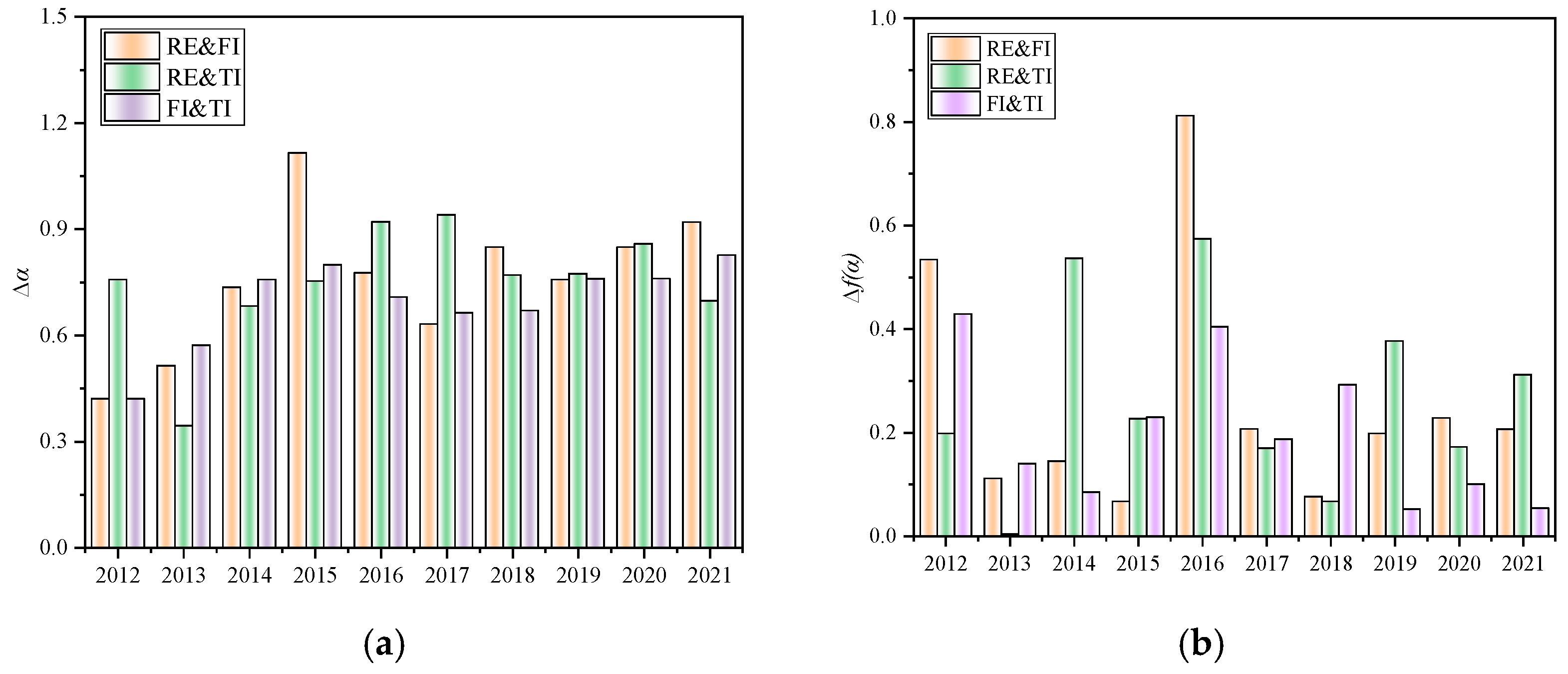
The parameters of the multifractal spectrum also convey information about local fluctuations in many markets, especially the width difference $\Delta \alpha$ and height difference $\Delta f\left(\alpha \right)$ of the multifractal spectrum. The fractal-spectrum analysis of cross-correlation was similar to that of the single time series. The $\Delta \alpha ={\alpha }_{max}-{\alpha }_{min}$ represents the dispersion of the distribution. The $\Delta \alpha =0$ corresponds to a completely uniform distribution. The larger $\Delta \alpha$ indicates that the distribution of the time series was more uneven and the cross-correlation fluctuations between the indices were more intense. The $\Delta f\left(\alpha \right)=f\left({\alpha }_{min}\right)-f\left({\alpha }_{max}\right)$ conveys the degree of local fluctuations of cross-correlation. Some studies have also pointed out that $\Delta f\left(\alpha \right)$ represents the number of occurrences of the singular index value, reflecting the proportion of the sequence signals at the peak and trough positions. The higher the $\left|\Delta f\left(\alpha \right)\right|$ is, the more chaotic the local fluctuations of the cross-correlation are.

Taking the overall sample as an example, the $\Delta \alpha$ and $\left|\Delta f\left(\alpha \right)\right|$ among the TI, FI, and RE were calculated and are listed in

Table 2. Parameters of multifractal spectrum.

Variable	${\mathit{\alpha }}_{\mathit{m}\mathit{i}\mathit{n}}$	${\mathit{\alpha }}_{\mathit{m}\mathit{a}\mathit{x}}$	$\mathbf{\Delta }\mathit{\alpha }$	$\mathit{f}\left({\mathit{\alpha }}_{\mathit{m}\mathit{i}\mathit{n}}\right)$	$\mathit{f}\left({\mathit{\alpha }}_{\mathit{m}\mathit{a}\mathit{x}}\right)$	$\left|\mathbf{\Delta }\mathit{f}\left(\mathit{\alpha }\right)\right|$
RE and FI	0.3890	0.7857	0.3967	0.2521	0.3137	0.0615
RE and TI	0.2830	0.7988	0.5157	0.1637	0.2651	0.1014
FI and TI	0.3744	0.7911	0.4167	0.2746	0.2936	0.0190

. The parameters of the multifractal spectrum among the TI, FI, and RE were constantly changing, and their corresponding function densities were inconsistent. In terms of $\Delta \alpha$, the $\Delta \alpha$ of TI-RE was the largest, followed by the $\Delta \alpha$ value of FI-TI, and the $\Delta \alpha$ value of FI-RE was the smallest. The values of $\Delta \alpha$ prove that the interactive relation between the RE and TI was more complex and the degree of multifractal was stronger. On the contrary, the multifractal degree between the RE and FI was relatively weaker.

In terms of $\left|\Delta f\left(\alpha \right)\right|$, the $\left|\Delta f\left(\alpha \right)\right|$ value of RE-TI was the largest. This indicates that the local fluctuations of the cross-correlation between the RE and TI were more volatile, whereas the $\left|\Delta f\left(\alpha \right)\right|$ value of RE-FI and FI-TI were significantly smaller than that of TI-RE. This means that the local dislocations of the cross-correlation between the RE and FI as well as FI and TI were relatively simple.

The fractal-spectrum shape of the FI-RE was very similar to that of FI-TI. The difference between the value of $\Delta \alpha$ for FI-RE and that of FI-TI was 0.02, and the difference between the $\left|\Delta f\left(\alpha \right)\right|$ of FI-RE and that of FI-TI was 0.0425. From the perspective of fractal spectrum, the change trend of the interaction between the FI and RE was similar to that between the FI and TI. In comparison, the fractal-spectrum width of TI-RE was more 0.099 that of TI-FI and FI-RE, and the fractal-spectrum height was also more than 0.0399. These show that the cross-correlation between TI and RE was unstable and partially chaotic.

In addition, the changes in multifractal-spectrum parameters of cross-correlation among the TI, FI, and RE in different periods were also explored, including the $\Delta \alpha$ and $\left|\Delta f\left(\alpha \right)\right|$. The results are shown in Figure 8. Consistently, the multifractal spectrum of cross-correlation among the TI, FI, and RE also had time-varying characteristics. For the TI and RE, the value of $\Delta \alpha$ was higher in 2015–2018 and 2020, and the value of $\left|\Delta f\left(\alpha \right)\right|$ was higher in 2019, 2019, and 2021. For the FI-RE, the value of $\Delta \alpha$ was higher in 2015–2016 and 2020–2021, and the value of $\left|\Delta f\left(\alpha \right)\right|$ was higher in 2016 and 2020. For the FI-TI, the value of $\Delta \alpha$ was also higher in 2015–2016 and 2021, and the value of $\left|\Delta f\left(\alpha \right)\right|$ was higher in 2015–2016 and 2020. The parameter changes of the multifractal spectrum among the TI, FI, and RE were similar.

It is worth noting that the parameter change of the multifractal spectrum also presented the characteristics of time delay. Although the stock-market crash occurred in 2015, the value of $\Delta \alpha$ and $\left|\Delta f\left(\alpha \right)\right|$ among the TI, FI, and RE remained at a higher level in the years following 2015. Similarly, the COVID-19 pandemic, which began at the end of 2019, kept the global economy in a sustained downturn, and the value of $\left|\Delta f\left(\alpha \right)\right|$ in 2019 and the following years also remained at a higher level. It can be concluded that the multifractal-spectrum parameters of the TI, FI, and RE changed significantly during the crisis periods and the subsequent periods.

5. Conclusions

The research results of the denoising analysis show that wavelet-threshold denoising can remove some noise information of technological-innovation, financial-market, and real-economy indices to improve the availability of effective information. Compared with the traditional denoising method, the effect of wavelet-threshold denoising is significantly more effective. After denoising, the volatility agglomeration of technological-innovation, financial-market, and real-economy indices was significantly reduced and the stability was improved. This was helpful for this study to observe a more authentic and reliable fluctuation relationship among technological-innovation, financial-market, and real-economy indices.

Several valuable findings were obtained from the study of the cross-correlation fractal between technological-innovation, financial-market, and real-economy indices, which were mainly manifested in the multiplicity, time-varying memory, and singularity of fractal characteristics. Firstly, the Hurst value of cross-correlation among technological-innovation, financial-market, and real-economy indices showed a decreasing trend with the increase in the fluctuation order. This means that the cross-correlation among them presented obvious multifractal characteristics rather than single-fractal characteristics. Secondly, the cross-correlation among technological-innovation, financial-market, and real-economy indices demonstrated the phenomenon of long memory, that is, the interaction between them had a long-term correlation in most periods. Locally, when the fluctuation was small, the cross-correlation among the three indices showed the characteristics of continuity. In the period of great fluctuation, the cross-correlation between them may have had the characteristics of anti-persistence, among which the cross-correlation between technological-innovation and real-economy indices had the strongest anti-persistence. Thirdly, the shape of the multifractal spectrum among the indices of technological innovation, the financial market, and the real economy were all parabola-like shapes with the opening facing down, which confirms the cross-correlation multifractal characteristics from the perspective of the fractal spectrum. In contrast, the width difference in the cross-correlation multifractal spectrum between the technological-innovation and real-economy indices was the largest, which indicates that the interaction between technological innovation and the real economy was more complex. Similarly, the height difference of the fractal spectrum between technological-innovation and real-economy indices was also the largest, which reflects the high degree of local chaos and instability of the interaction between the two.

In addition, it was found that the Hurst value and fractal spectrum of cross-correlation among the three indices were obviously different in different periods, but the change trend of the fractal characteristics among the three indices was roughly similar over time. The fractal characteristics of the crisis events during the period of occurrence and the following years were significantly strengthened, which indicates that the interaction between the three indices may have had a certain time delay and continuity.

Based on the study above, the research results are of great significance to investors and administrative departments. For investors, the conclusions will help them to realize the nonlinear dependence and potential dynamic mechanism between the three industries and have a deeper understanding of the linkage relationship and information transmission among the industries so as to provide investors with a decision-making basis. For economic policymakers, the fractal characteristics of interaction can help them understand the transmission and diffusion of market risks, deeply consider the important factors affecting the healthy growth of the real economy, and carry out policy regulation and management in a timely manner.

There are still many areas for in-depth discussion on the interaction between technological innovation, financial markets, and the real economy. For example, according to the different multifractal characteristics, how to control the risk diffusion in practice will be the focus of our future research, and the optimization of parameters also needs to be explored further.