Dynamical Analysis of Generalized Tumor Model with Caputo Fractional-Order Derivative

Abstract

In this study, we perform a dynamical analysis of a generalized tumor model using the Caputo fractional-order derivative. Tumor growth models are widely used in biomedical research to understand the dynamics of tumor development and to evaluate potential treatments. The Caputo fractional-order derivative is a mathematical tool that is recently being applied to model biological systems, including tumor growth. We present a detailed mathematical analysis of the generalized tumor model with the Caputo fractional-order derivative and examine its dynamical behavior. Our results show that the Caputo fractional-order derivative provides a more accurate description of the tumor growth dynamics compared to classical integer-order derivatives. We also provide a comprehensive stability analysis of the tumor model and show that the fractional-order derivative allows for a more nuanced understanding of the stability of the system. The least-square curve fitting method fits several biological parameters, including the fractional-order parameter $\alpha$. In conclusion, our study provides new insights into the dynamics of tumor growth and highlights the potential of the Caputo fractional-order derivative as a valuable tool in biomedical research. The results of this study shall have significant implications for the development of more effective treatments for tumor growth and the design of more accurate mathematical models of tumor development.

1. Introduction

This century is characterized by a high frequency of advanced research and investigations involving fractional-order integrals and derivatives. For example, big data, artificial intelligence, and machine learning are the top trending topics in applied scientific research. To better understand them, we need fractional dynamics as well as fractional-order thinking [1]. In this article, we use the Caputo fractional-order derivative to analyze the tumor–macrophage model using real medical data due to the fact that the study of tumor–immune system interactions has been ranked as one of the most complicated and varied phenomena in the field. Various effector cells, including monocytes and macrophages, make up the immune system. Fast-acting effector cells that release cytokines that activate and attract other effector cells constitute the front line of defense against malignancies. These effector cells launch the immune response against transformed or tumor cells after they have been activated [2]. One type of white blood cell in the body, macrophages, is responsible for squishing invading germs in the tissues. They assist in the repair of damaged tissue as well.

Recent research on tumor–macrophage interaction systems [3,4] shows that macrophages can perform both anti-tumor and pro-tumor activities, denoted by $M_1$ designating macrophages of type-1 cells called anti-tumor macrophages, and $M_2$ designating macrophages of type-2 cells called pro-tumor macrophages [5]. Furthermore, in [6], it is proposed that re-polarizing macrophages towards these traditionally activated anti-tumor cells ($M_1$) is a successful treatment for tumor eradication. Tumors, on the other hand, have a reputation for being extremely lethal. According to a 2015 estimate by the World Health Organization, the global incidence of cancer and other tumors is expected to increase by as much as 70 percent over the next two decades. As a result, a lot of effort is required to keep tumors under control. Because of this, there has been an explosion of theoretical and practical information regarding cancer as well as the underlying mechanisms of tumor–immune interaction dynamics [7,8,9,10].

The immune system plays a vital role in eliminating cancer cells. T cells (including CD$4^{+}$ T cells and CD$8^{+}$ T cells), B cells, macrophages, and natural killer (NK) cells are among the most vital components of the immune system [11]. Innate and adaptive immune responses rely heavily on macrophages. These cells populate the tumor microenvironment in the greatest numbers. Scientific studies have demonstrated that macrophages are particularly effective at destroying cancer cells. It is also crucial to focus on macrophages while developing novel oncological therapies. By blocking CSF1 receptors on macrophages using antibodies and small molecule medicines, tumor reduction can be achieved as a therapeutic goal. However, peripheral events in the tumor microenvironment are both complicated and dynamic. Because of this, developing strategies for curing or managing cancer is a daunting challenge. Tumor–immune dynamics is a field that greatly benefits from mathematical modeling because it allows researchers to better understand the complex interaction between immune cells and cancer cells. Mathematical models have been helpful to many scientists who are trying to unravel the mysteries of cancer development. Banerjee and Sarkar [12] are one group that has considered the delay-induced tumor–immune system model and cancerous tumor progression. The mathematical model of the interaction between tumor cells and macrophages has been investigated. Furthermore, in [13], the authors suggest a tumor growth model that takes into account the impact of radiotherapy by building it on the foundation of tumor radio-biologic pathways. They are looking into how radiotherapy for tumors can be improved by re-oxygenating hypnotized cells. Another study [14] used GWN to assess the quality of interactions between tumor cells and immune cells, as well as the efficacy of chemotherapy. By using an integer-order differential equation system, Eftimie and Barelle [15] modeled the dynamics of interactions between lung cancer and macrophages of varying phenotypes. For DNA damage and autophagy in lung cancer, Sarmah et al. [16] developed a seven-dimensional mathematical model. They also did a parameter recalibration analysis and a local and global sensitivity analysis to have a better understanding of the system dynamics.

In order to gain an understanding of the intricate workings of the tumor–macrophage interaction system, a significant amount of research has been conducted in this area [17,18,19]. The majority of the research work that is performed on tumor–macrophage interaction models is carried out with the use of integer-order differential equations. In the realm of biology, the idea of fractional-order differential equations with time delay has been applied often during the past few decades [20,21,22,23]. This is only due to the fact that models of biological systems developed by differential equations with fractional order display more realistic results and are more accurate for the description of hereditary and memory properties of the system in comparison to models described by integer-order differential equations. This is the only reason why this is a rare one. Nearly every mathematical model of a biological system has some form of long-range historical memory. This might take the form of a delay caused by the incubation period before vectors become infectious, a delay in the activation of effector cells such as macrophages by tumor interaction, or something along those lines.

For 300 years, only mathematicians, physicists, and engineers have had any need for fractional calculus. Fractional operations have traditionally been used in the traditional fields of commerce, healthcare, physics, synchronization of unstable systems, atmospheric ocean problems, fractal dynamics, geology, remote sensing, heat diffusion models, predatory species, epidemiology, and biology. Recent years have seen the introduction of a number of distinct fractional-order epidemiological models that are founded on the Caputo differential operator. Either the researchers have made new models, or they have shown that the existing models work better when the Caputo operator is used to look at them. A fractional-order Gompertz model was developed by researchers in [24], and they showed that the fractional-order Gompertz model demonstrated a better fit to the available real data when the order of the fractional derivative is taken as $0.68$ as compared to a model of integer-order. This was demonstrated by citing the study in which the fractional-order Gompertz model was developed. In the article [25], the authors investigate the stability features of a fractional-order model of the interaction between the immune system and tumors. In the article [26], researchers suggested a fundamental and straightforward fractional-order model to explore and investigate the dynamical behavior of the tumor–immune interaction system.

2. Advantages of Fractional Epidemic Models

Fractional epidemic models are mathematical models that use fractional calculus to describe the spread of infectious diseases. Here are some advantages of using fractional epidemic models:

• Improved accuracy: Fractional calculus allows for more accurate modeling of complex systems that cannot be easily described by traditional integer-order differential equations. This leads to more accurate predictions of disease dynamics and better decision making in public health;
• Flexibility: Fractional models can be adapted to fit a variety of data sets, including nonlinear and non-stationary data. This allows for a more flexible and adaptable approach to modeling infectious disease spread;
• Early detection: Fractional models can help detect disease outbreaks earlier than traditional models, which rely on historical data. This allows for more rapid implementation of control measures and containment strategies;
• Capturing long-term memory: Fractional models can account for long-term memory effects, such as the influence of previous outbreaks or social interactions, that may affect the spread of disease. This can lead to a more accurate description of disease dynamics and better prediction of future outbreaks;
• Improving public health policies: Fractional models can be used to evaluate the effectiveness of different public health policies and interventions, such as vaccination programs or social distancing measures. This allows policymakers to make informed decisions based on data and modeling results.

3. Why Caputo Operator?

Traditional models make use of local differential and integral operators; however, these operators neglect the specifics of the epidemic that is being researched. Because of this, the memory characteristics of the underlying system are not taken into account by standard calculus. Recent research has demonstrated that nonlocal operators are preferable to classical ones. As a result, these operators are the only option for including memory effects in a deterministic model of the epidemic. Recently, in the scientific literature, a number of various epidemic models for the infection caused by the interaction between tumors and macrophages have been presented.

The fractional-order differential operators have been applied in the development of a good number of them, with Caputo being the one that is used the majority of the time. On the other hand, the vast majority of study articles hardly ever offer an explanation for why the Caputo operator was applied in the research. In this regard, we made an attempt to describe some of the important reasons why one should keep in mind the Caputo operator while modeling an infectious disease using nonlinear differential equations. These reasons are discussed in more detail below, along with other important justifications for the use of the fractional-order operator in the tumor–macrophage interaction model considered in this research work.

• By simply replacing $n\in \mathbb{N}$ with $\alpha \in \mathbb{C}$, Re$\left(\alpha \right)>0$, the famous Riemann–Liouville integral formula is derived from the Cauchy formula for repeated integration; this fractional integral formula is now the foundation for the development of various numerical methods used to solve fractional ordinary and partial differential equations;
• Caputo’s version of classical epidemiological models has been successfully applied in recent works [27,28,29,30], coupled with specifics for the presence of a unique solution and stability analysis. There, numerical simulations were used to show why the Caputo variant is better than the traditional one;
• Recent publications in the field of epidemiology show that traditional models were not able to accurately capture the complicated and chaotic dynamics of the spread of infections. Instead, real data about the epidemic, mostly from reliable sources such as the World Health Organization and empirically published papers, were used to verify and confirm the Caputo versions;
• Furthermore, when we use Caputo’s differential operator to examine the disease’s behavior under different biological parameter values, we obtain a clear picture of the basic reproductive number, which explains the average number of secondary infections produced when an infectious individual enters a completely susceptible class. Consider, for instance, [31,32] and the majority of the references therein.

In this paper, we generalize an integer-order tumor–macrophage interaction model given by S. Yaqin et al. [5] by introducing the Caputo-type fractional-order derivative. The mathematical model proposed by S. Yaqin et al. [5] is given by the following three nonlinear ordinary differential equations:

$$\begin{array}{c}\hfill \begin{array}{cc}\hfill {\displaystyle \frac{dT}{dt}}& =aT(1-bT)-fT{M}_1+gT{M}_2,\hfill \\ \hfill {\displaystyle \frac{d{M}_1}{dt}}& =e_{1}T{M}_1-d_1{M}_1-r_1{M}_1+r_2{M}_2,\hfill \\ \hfill {\displaystyle \frac{d{M}_2}{dt}}& =e_{2}T{M}_2-d_2{M}_2+r_1{M}_1-r_2{M}_1,\hfill \end{array}\end{array}$$

(1)

where T, $M_1$, and $M_2$ represent the populations of tumor cells, anti-tumor cells ($M_1$ type of cells), and pro-tumor cells ($M_2$ type of cells), respectively. Furthermore, $a,b,f,g,e_1,d_1,r_1,r_2,e_2$, and $d_2$ are all positive constants. For biological presumptions of model (1) and its dimensionless form, see [5]. The parameters of the above model are mentioned in

Table 1. System parameters and variables used for numerical simulation.

Parameters	Values	Biological Interpretation	Dimensionless Form	Source
$T\left(0\right)$	${10}^6$ cells (c)	No. of initial T cells	$x_0$
$M_1\left(0\right)$	${10}^6$ cells	No. of initial $M_1$ cells	$y_0$
$M_2\left(0\right)$	${10}^6$ cells	No. of initial $M_2$ cells	$z_0$
a	0.565/day	Growth rate of T cells	${\varrho }^{{}^{\prime }}$
$b^{-1}$	$2\times {10}^9$/cells	Environmental carrying capacity	${\displaystyle \frac{1}{{\beta }^{{}^{\prime }}}}$
$d_1$	0.2/day (d)	Mortality rate of $M_1$ cells	${\mu }_1^{{}^{\prime }}$
$d_2$	0.2/day (d)	Mortality rate of $M_2$ cells	${\mu }_2^{{}^{\prime }}$	[33]
f	$2\times {10}^{-6}$/cd	Death rate of T cells by $M_1$ cells	${\delta }^{{}^{\prime }}$
g	${10}^{-7}$/cd	Death rate of T cells by $M_2$ cells	${\eta }^{{}^{\prime }}$
$e_1$	${10}^{-6}$/cd	Enabling rate of $M_1$ by T cells	${\zeta }_0^{{}^{\prime }}=1$
$e_2$	$9\times {10}^{-7}$/cd	Enabling rate of $M_2$ by T cells	${\zeta }^{{}^{\prime }}$
$r_1$	0.05/day	$M_1$ to $M_2$ conversion rate	${\gamma }_1^{{}^{\prime }}$
$r_2$	0.04/day	$M_2$ to $M_1$ conversion rate	${\gamma }_2^{{}^{\prime }}$

. Now, our proposed Caputo-based fractional-order tumor–macrophage interaction model in dimensionless form is given by

$$\begin{array}{c}\hfill \begin{array}{cc}\hfill D_{0,t}^{\alpha }x\left(t\right)& ={\varrho }^{{}^{\prime }}x\left(t\right)(1-{\beta }^{{}^{\prime }}x\left(t\right))-{\delta }^{{}^{\prime }}x\left(t\right)y\left(t\right)+{\eta }^{{}^{\prime }}x\left(t\right)z\left(t\right),\hfill \\ \hfill D_{0,t}^{\alpha }y\left(t\right)& ={\zeta }_0^{{}^{\prime }}x\left(t\right)y\left(t\right)-{\mu }_1^{{}^{\prime }}y\left(t\right)-{\gamma }_1^{{}^{\prime }}y\left(t\right)+{\gamma }_2^{{}^{\prime }}z\left(t\right),\hfill \\ \hfill D_{0,t}^{\alpha }z\left(t\right)& ={\zeta }^{{}^{\prime }}x\left(t\right)z\left(t\right)-{\mu }_2^{{}^{\prime }}z\left(t\right)+{\gamma }_1^{{}^{\prime }}y\left(t\right)-{\gamma }_2^{{}^{\prime }}z\left(t\right),\hfill \end{array}\end{array}$$

(2)

where $\alpha >0$ is the order of derivative and $\alpha \in (n-1,n)$,$n\in \mathbb{N}$. Furthermore, $x\left(t\right)$, $y\left(t\right)$ and, $z\left(t\right)$ represent the population size of tumor cells, $M_1$ cells, and $M_2$ cells, respectively, at time t. For the biological meaning of parameters involved in our proposed models, see [5].

The remaining sections of the paper are presented as follows: In Section 4, we introduce some fundamental ideas, definitions, and theorems of fractional-order derivatives that were employed in the study of the model. Both the existence and the uniqueness of solutions to the model are examined in Section 5. In Section 6, we fitted some biological parameters and found the best value for the fractional order $\alpha$ with the help of real medical data. We determined equilibrium states, performed linearization, and conducted a stability analysis of the Caputo model in Section 7. The results of the numerical simulation are discussed in Section 8. The article concludes with some final thoughts and potential next steps in Section 9.

4. Preliminaries

This section reviews some important definitions and concepts of fractional-order derivatives required to analyze our proposed model based on the Caputo fractional-order operator.

Definition 1

([34]). Consider a function $\phi \left(t\right)$, $t>0$. The Riemann–Liouville integral operator $\phi \left(t\right)$ of order α is defined by the following:

$$\begin{array}{c}\hfill I^{\alpha }\phi \left(t\right)={\int }_0^t{\displaystyle \frac{{(t-r)}^{\alpha -1}}{\mathsf{\Gamma }\left(\alpha \right)}}\phi \left(r\right)dr,\end{array}$$

where $n:=\lceil \alpha \rceil$ is the smallest integer $\ge \alpha$ and for $n=1$, the above integral operator reduces to first-order integral operator.

The fractional-order derivative of the above function is defined by the following:

$$\begin{array}{c}\hfill D^{\alpha }\phi \left(t\right)=I^{n-\alpha }{D}^{\left(n\right)}\phi \left(t\right),\end{array}$$

where $\left(D={\displaystyle \frac{d}{dt}}\right)$.

Definition 2

([35]). Consider a real valued function $\phi \left(t\right)$, $t>0$. The Caputo-type fractional derivative of order $\alpha >0$ is given by the following:

$$\begin{array}{c}\hfill D^{\alpha }\phi \left(t\right)={\displaystyle \frac{1}{\mathsf{\Gamma }(n-\alpha )}}{\int }_0^t{(t-r)}^{n-\alpha -1}{\phi }^{\left(n\right)}\left(r\right)dr,\end{array}$$

where n is an integer, $\alpha \in (n-1,n)$ and $D^{\alpha }\phi \left(t\right)$ denotes the Caputo-type fractional-order operator ${}^C{D}_{0,t}^{\alpha }\phi \left(t\right).$

Theorem 1

([36]). Consider a system of fractional-order differential equations:

$$\begin{array}{c}\hfill D_b^{\alpha }\phi \left(t\right)=\phi (t,Y\left(t\right)),Y\left(t_0\right)=Y_0.\end{array}$$

(3)

Let $J\left(Y^{*}\right)$ be the Jacobian matrix of system (3) estimated at the equilibrium point $Y^{*}$. The following statements will always be true:

1

The equilibrium point $Y^{*}$ is locally asymptotically stable if and only if all eigenvalues ${\lambda }_i$, $i=1,2,3,\dots ,n$ of Jacobian matrix $J\left(Y^{*}\right)$ satisfy $|arg{\lambda }_i|>\alpha \pi /2$;

2

The equilibrium point $Y^{*}$ is stable if and only if all eigenvalues ${\lambda }_i$, $i=1,2,3,\dots ,n$ of jacobian matrix $J\left(Y^{*}\right)$ satisfy $|arg{\lambda }_i|\ge \pi /2$ and eigenvalues with $|arg{\lambda }_i|$=$\alpha \pi /2$ have same algebraic and geometric multiplicity;

3

The equilibrium point $Y^{*}$ is unstable if and only if there exist eigenvalues ${\lambda }_i$, for some $i=1,2,3,\dots ,n$ of Jacobian matrix $J\left(Y^{*}\right)$ such that $|arg{\lambda }_i|<\alpha \pi /2$.

5. Existence and Uniqueness of Solutions of Caputo System

In this section, we prove the existence, uniqueness, and positivity of the solutions of the fractional-order tumor model (2) with the help of the following lemma and definitions.

Lemma 1

([37]). Consider the system of equations given by (2):

$$\begin{array}{c}\hfill \begin{array}{cc}\hfill D^{\alpha }x\left(t\right)& ={\varrho }^{{}^{\prime }}x(1-{\beta }^{{}^{\prime }}x)-{\delta }^{{}^{\prime }}xy+{\eta }^{{}^{\prime }}xz,\hfill \\ \hfill D^{\alpha }y\left(t\right)& =xy-{\mu }_1^{{}^{\prime }}y-{\gamma }_1^{{}^{\prime }}y+{\gamma }_2^{{}^{\prime }}z,\hfill \\ \hfill D^{\alpha }z\left(t\right)& ={\zeta }^{{}^{\prime }}xz-{\mu }_2^{{}^{\prime }}z+{\gamma }_1^{{}^{\prime }}y-{\gamma }_2^{{}^{\prime }}z.\hfill \end{array}\end{array}$$

We will choose the initial conditions as follows: $x\left(t_0\right)=x_0$, $y\left(t_0\right)=y_0$, $z\left(t_0\right)=z_0$.

The system (2) can be written in the following form:

$$\begin{array}{c}\hfill D^{\alpha }Y\left(t\right)=R_{1}Y\left(t\right)+x\left(t\right)R_{2}Y\left(t\right),Y\left(t_0\right)=Y_0,\end{array}$$

(4)

where, $Y\left(t\right)$= $\left(\begin{array}{c}x\left(t\right)\\ y\left(t\right)\\ z\left(t\right)\end{array}\right),$ $Y\left(0\right)$= $\left(\begin{array}{c}x\left(0\right)\\ y\left(0\right)\\ z\left(0\right)\end{array}\right),$ $R_1$= $\left(\begin{array}{ccc}{\varrho }^{{}^{\prime }}& 0& 0\\ 0& -{\mu }_1^{{}^{\prime }}-{\gamma }_1^{{}^{\prime }}& {\gamma }_2^{{}^{\prime }}\\ 0& {\gamma }_1^{{}^{\prime }}& -{\mu }_2^{{}^{\prime }}-{\gamma }_2^{{}^{\prime }}\end{array}\right),$ and

$R_2$= $\left(\begin{array}{ccc}-{\varrho }^{{}^{\prime }}{\beta }^{{}^{\prime }}& -{\delta }^{{}^{\prime }}& {\eta }^{{}^{\prime }}\\ 1& 0& 0\\ 0& 0& {\zeta }^{{}^{\prime }}\end{array}\right)$.

The following definitions are required for the existence and uniqueness of solutions of system (4) [37,38].

Definition 3.

Let us consider $\mathbf{C}[0,\theta ]$ to be a class of continuous column vector $Y\left(t\right)$, with components (functions) $x\left(t\right),y\left(t\right),z\left(t\right)\in \mathbf{C}[0,\theta ]$, as the class of continuous function on the interval $[0,\theta ]$. Then, the norm of $Y\in \mathbf{C}[0,\theta ]$ is given by the following:

$$\begin{array}{c}\hfill \parallel Y\parallel =\underset{t}{sup}|exp(-nt)x\left(t\right)|+\underset{t}{sup}|exp(-nt)y\left(t\right)|+\underset{t}{sup}|exp(-nt)z\left(t\right)|.\end{array}$$

Definition 4.

$Y\in \mathbf{C}[0,\theta ]$ is a column vector that satisfies the initial value problem (4) and, therefore, is the solution of the system of equations given by (4) if

1.

$(t,Y\left(t\right))\in D$, $t\in [0,\theta ]$. Where $D=[0,\theta ]\times U$, $U=[(x,y,z)\in R_{+}^3:|x|\le u,|y|\le v,|z|\le w]$, and $u,v,w$ are positive constants;

2.

$Y\left(t\right)$ satisfies the system (4).

Theorem 2.

The system of equations given by (4) has a unique solution $Y\in \mathbf{C}[0,\theta ]$.

Proof. 

With the help of properties of fractional-order derivatives, the system of fractional-order differential Equation (4) can be written as follows:

$$\begin{array}{c}\hfill I^{1-\alpha }{\displaystyle \frac{d}{dt}}Y\left(t\right)=R_{1}Y\left(t\right)+x\left(t\right)R_{2}Y\left(t\right).\end{array}$$

Operating $I^{\alpha }$ on both sides, we have

$$\begin{array}{c}\hfill Y\left(t\right)=Y\left(0\right)+I^{\alpha }[R_{1}Y\left(t\right)+x\left(t\right)R_{2}Y\left(t\right)].\end{array}$$

(5)

Now, let us consider an operator $G:\mathbf{C}[0,\theta ]⟶\mathbf{C}[0,\theta ]$, which is defined by the following:

$$\begin{array}{c}\hfill G\left[Y\left(t\right)\right]=Y\left(0\right)+I^{\alpha }[R_{1}Y\left(t\right)+x\left(t\right)R_{2}Y\left(t\right)].\end{array}$$

(6)

Therefore, we have

$$\begin{array}{cc}\hfill exp(-nt)\left[G\right[Y\left(t\right)]-G[Z\left(t\right)\left]\right]& \le exp(-nt)I^{\alpha }[R_1[Y\left(t\right)-Z\left(t\right)]+x\left(t\right)R_2[Y\left(t\right)-Z\left(t\right)]]\\ & \le {\displaystyle \frac{1}{\mathsf{\Gamma }\left(\alpha \right)}}{\int }_0^t{(t-c)}^{\alpha -1}exp(-n(t-c))\left[Y\left(c\right)-Z\left(c\right)\right]\\ & exp(-nc)[R_1+u{R}_2]ds\\ & \le {\displaystyle \frac{(R_1+u{R}_2)}{n^{\alpha }}}\parallel Y\left(t\right)-Z\left(t\right)\parallel {\int }_0^t{\displaystyle \frac{c^{\alpha -1}}{\mathsf{\Gamma }\left(\alpha \right)}}\end{array}$$

$$\begin{array}{c}\hfill \Rightarrow \parallel G[Y\left(t\right)-Z\left(t\right)]\parallel \le {\displaystyle \frac{R_1+u{R}_2}{n^{\alpha }}}\parallel Y\left(t\right)-Z\left(t\right)\parallel .\end{array}$$

(7)

Let us choose the value of n, such that $R_1+u{R}_2<n^{\alpha }$ ( see [39]). Then, from (7), we obtain

$$\begin{array}{c}\hfill \parallel G\left[Y\right(t)-Z(t\left)\right]\parallel <\parallel Y\left(t\right)-Z\left(t\right)\parallel .\end{array}$$

The operator G given by (6) has a fixed point. Consequently, system (5) has a unique solution $Y\in \mathbf{C}[0,\theta ]$. Now from system (5), we have

$$\begin{array}{c}\hfill Y\left(t\right)=Y\left(0\right)+{\displaystyle \frac{t^{\alpha }}{\mathsf{\Gamma }(\alpha +1)}}[R_{1}Y\left(0\right)+x\left(0\right)R_{2}Y\left(0\right)]+I^{\alpha +1}[R_1{Y}^{{}^{\prime }}\left(t\right)+x^{{}^{\prime }}\left(t\right)R_{2}Y\left(t\right)+x\left(t\right)R_2{Y}^{{}^{\prime }}\left(t\right)],\end{array}$$

and

$$\begin{array}{cc}\hfill exp(-nt)Y^{{}^{\prime }}\left(t\right)& =exp(-nt)[{\displaystyle \frac{t^{\alpha -1}}{\mathsf{\Gamma }\left(\alpha \right)}}[R_{1}Y\left(0\right)+x\left(0\right)R_{2}Y\left(0\right)]+I^{\alpha }[R_1{Y}^{{}^{\prime }}\left(t\right)\\ & +x^{{}^{\prime }}\left(t\right)R_{2}Y\left(t\right)+x\left(t\right)R_2{Y}^{{}^{\prime }}\left(t\right)\left]\right].\end{array}$$

Therefore, from the above analysis, it can be deduced that $Y^{{}^{\prime }}\left(t\right)\in \mathbf{C}[0,\theta ]$.

Again, from system (5), we have

$$\begin{array}{c}\hfill D^{\alpha }Y\left(t\right)=R_{1}Y\left(t\right)+x\left(t\right)R_{2}Y\left(t\right),\end{array}$$

and

$$\begin{array}{c}\hfill Y\left(0\right)=Y_0+I^{\alpha }[R_{1}Y\left(t\right)+x\left(t\right)R_{2}Y\left(t\right)].\end{array}$$

Hence, the system of equations given by (5) is equivalent to the system of equations given by (2). □

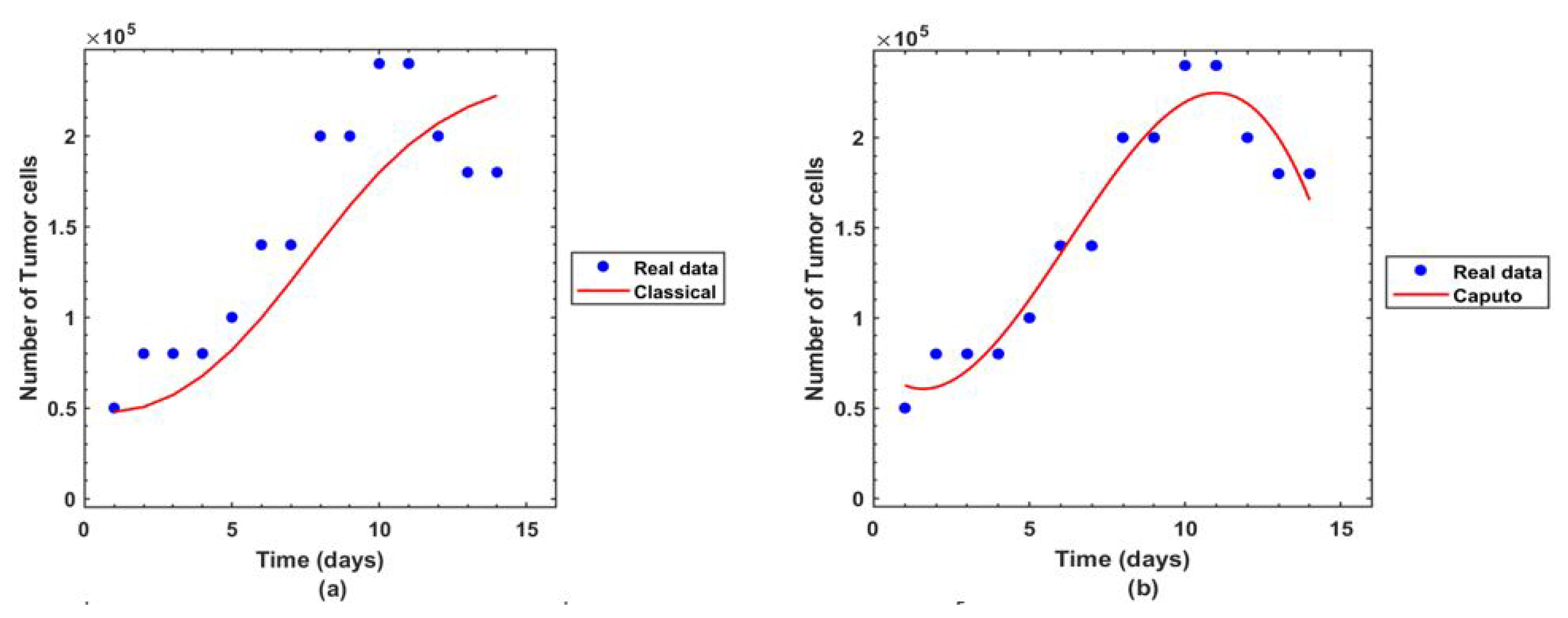
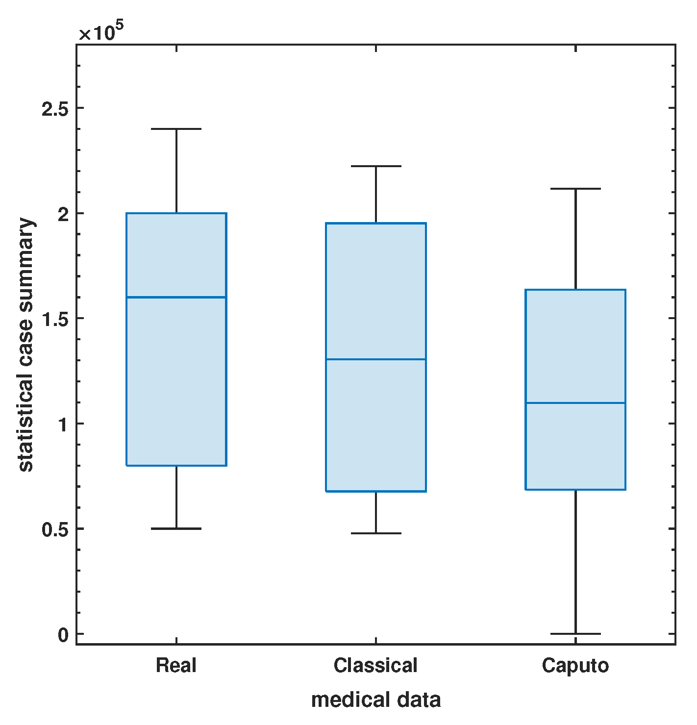
6. Fitting of Biological Parameters with Real Medical Data

When working with mathematical models that make use of real data, the most important issue that has to be addressed is validating the models and finding the ideal values for the parameters. This is due to the fact that the majority of the time, the parameter values cannot be precisely determined from the obtained data. It is absolutely necessary to acquire fitted parameter values for the model in question. By taking into account both the early behavior of the epidemic as well as the demographic aspects that are linked with the disease, it is possible to simply compute some of the parameters that are associated with epidemics. The values of the parameters can also be obtained from the existing literature, which can then be used as a guide for creating estimations, despite the fact that the latter technique can occasionally cause the results to behave in an unpredictable way. It is vital to discover the right biological parameters that characterize the cells in order to collect the data for an authentic and reliable number of tumor cells. This will allow the data to be collected. These kinds of real-life examples can be provided for a length of time spanning from days, to weeks, to months, and even years at a time. There is a chance that the conclusion is not accurate as a result of the inaccuracies that were introduced during the data analysis. Although there are a number of approaches for estimating parameter values, the least-squares method is the most commonly used. This is despite the fact that the literature contains a number of different methods that can be used.

While many cancer models have been identified and validated, parameter estimation remains a significant challenge. To make sure the proposed model is the best possible model for expressing cancer, its parameters are estimated using real data and kept within reasonable ranges. Most importantly, parameter estimation enables the acquisition of parameter values that are unique to the developed model rather than using parameter values obtained for other types of cancer models found in the associated literature. Using the data of a patient with lung cancer (a tumor in the lungs) treated at the Kayseri Erciyes University Hospital, the appropriate parameters have been attempted to be fitted using the least-squares curve fitting technique. The data collected from the patient’s lung tumor cells over the course of 14 days (15 September–28 September 2022), as referred to in [40], were used to perform a least-squares curve fit for the model’s two parameters. The best-fit parameter values were determined by attempting to reduce the average absolute relative error between the real lung cancer patient tumor cell data and the solution of models for the tumor class.

Table 2. The description of the parameters with both fixed and best-fitted values.

Parameter	Explanation	(Caputo)	(Classical)	Source
$T\left(0\right)$	Initial T cells	50,000	50,000	fixed
$M_1\left(0\right)$	Initial $M_1$ cells	2,060,000	2,060,000	fixed
$M_2\left(0\right)$	Initial $M_2$ cells	80,000	80,000	fixed
$\alpha$	Fractional order	7.156 × ${10}^{-1}$	1	fitted
a	Growth rate of T cells	0.565	0.565	fixed
b	Environmental carrying capacity	1.15497 × ${10}^{-8}$	3.53497 × ${10}^{-6}$	fitted
$d_1$	Mortality rate of $M_1$ cells	0.2	0.2	fixed
$d_2$	Mortality rate of $M_2$	0.2	0.2	fixed
f	cells	3.20516 × ${10}^{-9}$	2.80857 × ${10}^{-7}$	fitted
$e_1$	Enabling rate of $M_1$ by T	1 × ${10}^{-6}$	1 × ${10}^{-6}$	fixed
$e_2$	Enabling rate of $M_2$ by T cells	9 × ${10}^{-7}$	9 × ${10}^{-7}$	fixed
$r_1$	$M_1$ to $M_2$ conversion rate	0.05	0.05	fixed
$r_2$	$M_1$ to $M_2$ conversion rate	0.04	0.04	fixed

lists the model’s biological parameters and their best-fitted values amongst the optimized fractional-order parameter $\alpha$ for the Caputo operator, which is computed to be ≈0.75156. The actual tumor values are depicted as solid blue circles in Figure 1, while the best-fitting model curve is shown as a solid red line. It is simple to see that the fitted curve for the Caputo operator agrees with real medical data more efficiently than the classical one. It demonstrates the superiority and utility of the fractional-order model over the integer model. Furthermore, the important statistical case summary shown in Figure 2 shows no outlier in any of the boxes.

The method of least-squares uses the idea of minimizing residuals between available infections for real data ${\overline{y}}_j=0,1,\dots ,n$ and the discrete points obtained with the suggested set of equations’ simulation $f(t_j,y_j)$ as given below:

$$\mathrm{Residual}={\displaystyle \frac{1}{N}}\sum _{j=0}^N\left|{\displaystyle \frac{{\overline{y}}_j-y_j}{{\overline{y}}_j}}\right|.$$

(8)

The aforementioned goal was reached by leveraging Wolfram Mathematica 12.1’s built-in NonlinearModelFit and ParametricNDSolve algorithms. Table 2 displays these adjusted values, while

Table 3. The fitted biological parameters with statistical measures.

Parameter	Estimate	Standard Error	t-Statistic	p-Value	Confidence Interval
$\alpha$	7.156 × ${10}^{-1}$	2.14317 × ${10}^{-6}$	3.2147	2.21216 × ${10}^{-3}$	{1.2372 × ${10}^{-5}$, 7.1729 × ${10}^{-5}$}
b	3.53497 × ${10}^{-6}$	7.08326 × ${10}^{-7}$	4.99061	3.14217 × ${10}^{-4}$	{1.99166 × ${10}^{-6}$, 5.07828 × ${10}^{-6}$}
f	2.80857 × ${10}^{-7}$	7.10913 × ${10}^{-8}$	3.95066	1.92551 × ${10}^{-3}$	{1.25963 × ${10}^{-7}$, 4.35752 × ${10}^{-7}$}

gives important statistical measurements for the estimated parameters, including standard error, t-statistic, p-value, and confidence interval.

In the existing literature [41,42,43], experimental data includes cell lines and animal data. Cell lines can forecast unconstrained growth, high-throughput screening, therapy response, and resistance. They are cheaper, simpler, and more reproducible. Cancer cell lines have restrictions. In vitro-grown tumors, subgroups become cell lines. However, the cancer subtype and level of tissue resemblance are typically unknown. This creates cancer cell lines that do not reflect human tumor diversity. Monolayer-grown cell lines lack the heterogeneity of tumor cells. Patient-derived xenograft cancer models improve on cancer cell line models, yet they have limitations. Mouse vaccination and medication validation require a long period of time, limiting their use in patient therapy. These models also have limitations in terms of pharmacological combinations and genetic manipulation, such as transgene or knockout studies. Primary cell cultures use cells directly from the tumor location and extensive pathology information to compare the culture’s features to those of the tumor. Primary cell culture predicts chemotherapeutic responses better.

7. Dynamical Analysis of Caputo System

7.1. Equilibria of the Caputo System

The equilibrium points of our proposed model (2) will be the same as the equilibrium points obtained from the model given in [5]. However, the stability and dynamical analysis of our proposed model will be distinct because, in this section, we analyzed the system of fractional-order derivatives by using Theorem 1 given in Section 4. The equilibrium points of system (2) are given by

i

$E_1=E_1(x_1,y_1,z_1)=E_1(0,0,0)$, the trivial equilibrium point;

ii

$E_2=E_2(x_2,y_2,z_2)=E_2\left({\displaystyle \frac{1}{{\beta }^{{}^{\prime }}}},0,0\right)$, the tumor-dominant equilibrium point;

iii

$E_3=E_3(x_3,y_3,z_3)=E_3\left(x_3,{\displaystyle \frac{{\varrho }^{{}^{\prime }}(1-{\beta }^{{}^{\prime }}{x}_3){\gamma }_2^{{}^{\prime }}}{{\delta }^{{}^{\prime }}{\gamma }_2^{{}^{\prime }}+{\eta }^{{}^{\prime }}(x_3-{\mu }_1^{{}^{\prime }}-{\gamma }_1^{{}^{\prime }})}},{\displaystyle \frac{{\varrho }^{{}^{\prime }}(1-{\beta }^{{}^{\prime }}{x}_3)({\mu }_1^{{}^{\prime }}+{\gamma }_1^{{}^{\prime }}-x_3)}{{\delta }^{{}^{\prime }}{\gamma }_2^{{}^{\prime }}+{\eta }^{{}^{\prime }}(x_3-{\mu }_1^{{}^{\prime }}-{\gamma }_1^{{}^{\prime }})}}\right)$, the positive interior equilibrium point.

The equilibrium point $E_3(x_3,y_3,z_3)$ is the positive interior equilibrium point of system (2), if the positivity conditions defined by Equation (5) in [5] are satisfied by $E_3(x_3,y_3,z_3)$. For the stability analysis of system (2), first, we linearize it at the general fixed point, which will help us in easing the analysis of model (2).

7.2. Linearization of Caputo System

Let us consider $E(\overline{x},\overline{y},\overline{z})$ as a general study state of system (2). Then, by using the linearization process on the system of fractional-order differential equations given by (2), we obtain:

$$\begin{array}{c}\hfill \begin{array}{cc}\hfill D^{\alpha }x\left(t\right)& =[{\varrho }^{{}^{\prime }}-2{\varrho }^{{}^{\prime }}{\beta }^{{}^{\prime }}\overline{x}-{\delta }^{{}^{\prime }}\overline{y}+{\eta }^{{}^{\prime }}\overline{z}](x-\overline{x})+{\delta }^{{}^{\prime }}\overline{x}(y-\overline{y})+{\eta }^{{}^{\prime }}\overline{x}(z-\overline{z}),\hfill \\ \hfill D^{\alpha }y\left(t\right)& =\overline{y}(x-\overline{x})+[\overline{x}-{\mu }_1^{{}^{\prime }}-{\gamma }_1^{{}^{\prime }}](y-\overline{y})+{\gamma }_2^{{}^{\prime }}(z-\overline{z}),\hfill \\ \hfill D^{\alpha }z\left(t\right)& ={\zeta }^{{}^{\prime }}\overline{z}(x-\overline{x})+{\gamma }_1^{{}^{\prime }}(y-\overline{y})+[{\zeta }^{{}^{\prime }}\overline{x}-{\mu }_2^{{}^{\prime }}-{\gamma }_2^{{}^{\prime }}](z-\overline{z}).\hfill \end{array}\end{array}$$

(9)

Therefore, the linearized system (9) in matrix form is given by the following:

$$\left(\begin{array}{c}{D}^{\alpha }x\left(t\right)\\ D^{\alpha }y\left(t\right)\\ D^{\alpha }z\left(t\right)\end{array}\right)=\left(\begin{array}{ccc}{\varrho }^{{}^{\prime }}-2{\varrho }^{{}^{\prime }}{\beta }^{{}^{\prime }}\overline{x}-{\delta }^{{}^{\prime }}\overline{y}+{\eta }^{{}^{\prime }}\overline{z}& {\delta }^{{}^{\prime }}\overline{x}& {\eta }^{{}^{\prime }}\overline{x}\\ \overline{y}& \overline{x}-{\mu }_1^{{}^{\prime }}-{\gamma }_1^{{}^{\prime }}& {\gamma }_2^{{}^{\prime }}\\ {\zeta }^{{}^{\prime }}\overline{z}& {\gamma }_1^{{}^{\prime }}& {\zeta }^{{}^{\prime }}\overline{x}-{\mu }_2^{{}^{\prime }}-{\gamma }_2^{{}^{\prime }}\end{array}\right)\left(\begin{array}{c}x-\overline{x}\\ y-\overline{y}\\ z-\overline{z}\end{array}\right).$$

7.3. Stability Analysis of Caputo System

Theorem 3.

The tumor-free equilibrium point $E_1(x_1,y_1,z_1)=E_1(0,0,0)$ is always unstable.

Proof. 

The Jacobian matrix of linearized system (9) at the equilibrium point $E_1(0,0,0)$ is given by the following:

$$\begin{array}{c}\hfill J_{E_1(0,0,0)}=\left(\begin{array}{ccc}{\varrho }^{{}^{\prime }}& 0& 0\\ 0& -{\mu }_1^{{}^{\prime }}-{\gamma }_1^{{}^{\prime }}& {\gamma }_2^{{}^{\prime }}\\ 0& {\gamma }_1^{{}^{\prime }}& -{\mu }_2^{{}^{\prime }}-{\gamma }_2^{{}^{\prime }}\end{array}\right).\end{array}$$

The eigenvalues of $J_{E_1(0,0,0)}$ are given by the roots of the characteristic equation:

$$\begin{array}{c}\hfill ({\varrho }^{{}^{\prime }}-\lambda )[(-{\mu }_1^{{}^{\prime }}-{\gamma }_1^{{}^{\prime }}-\lambda )(-{\mu }_2^{{}^{\prime }}-{\gamma }_2^{{}^{\prime }}-\lambda )-{\gamma }_1^{{}^{\prime }}{\gamma }_2^{{}^{\prime }}].\end{array}$$

Here, $\lambda ={\varrho }^{{}^{\prime }}>0$. ⇒$\left|arg\left(\lambda \right)\right|<{\displaystyle \frac{\alpha \pi }{2}}$.

Therefore, the equilibrium points $E_1(0,0,0)$ of system (2) are always unstable. □

Theorem 4.

The tumor-dominant equilibrium point $E_2\left({\displaystyle \frac{1}{{\beta }^{{}^{\prime }}}},0,0\right)$ of Caputo system (2) is locally asymptotically stable if ${\zeta }_1^{{}^{\prime }}<{\zeta }^{{}^{\prime }}<{\zeta }_0^{{}^{\prime }}$, where ${\zeta }_1^{{}^{\prime }}=\left({\mu }_1^{{}^{\prime }}+{\gamma }_1^{{}^{\prime }}+{\mu }_2^{{}^{\prime }}+{\gamma }_2^{{}^{\prime }}\right){\beta }^{{}^{\prime }}$ and ${\zeta }_0^{{}^{\prime }}=\left({\displaystyle \frac{{\gamma }_1^{{}^{\prime }}{\gamma }_2^{{}^{\prime }}{\beta }^{{}^{\prime }}}{1-({\mu }_1^{{}^{\prime }}+{\gamma }_1^{{}^{\prime }}){\beta }^{{}^{\prime }}}}+{\mu }_2^{{}^{\prime }}+{\gamma }_2^{{}^{\prime }}\right)$.

Proof. 

The Jacobian matrix of linearized system (9) at the equilibrium point $E_2\left({\displaystyle \frac{1}{{\beta }^{{}^{\prime }}}},0,0\right)$ is given by the following:

$$\begin{array}{c}\hfill J_{E_2\left({\displaystyle \frac{1}{{\beta }^{{}^{\prime }}}},0,0\right)}=\left(\begin{array}{ccc}-{\varrho }^{{}^{\prime }}& {\displaystyle \frac{{\delta }^{{}^{\prime }}}{{\beta }^{{}^{\prime }}}}& {\displaystyle \frac{{\eta }^{{}^{\prime }}}{{\beta }^{{}^{\prime }}}}\\ 0& {\displaystyle \frac{1}{{\beta }^{{}^{\prime }}}}-{\mu }_1^{{}^{\prime }}-{\gamma }_1^{{}^{\prime }}& {\gamma }_2^{{}^{\prime }}\\ 0& {\gamma }_1^{{}^{\prime }}& {\displaystyle \frac{{\zeta }^{{}^{\prime }}}{{\beta }^{{}^{\prime }}}}-{\mu }_2^{{}^{\prime }}-{\gamma }_2^{{}^{\prime }}\end{array}\right).\end{array}$$

The eigenvalues of $J_{E_2}$ are given by the following: $\lambda =-\varrho$ ⇒ $\left|arg\lambda \right|>{\displaystyle \frac{\alpha \pi }{2}}$ and $\left({\displaystyle \frac{1}{{\beta }^{{}^{\prime }}}}-{\mu }_1^{{}^{\prime }}-{\gamma }_1^{{}^{\prime }}-\lambda \right)$$\left({\displaystyle \frac{{\zeta }^{{}^{\prime }}}{{\beta }^{{}^{\prime }}}}-{\mu }_2^{{}^{\prime }}-{\gamma }_2^{{}^{\prime }}-\lambda \right)-{\gamma }_1^{{}^{\prime }}{\gamma }_2^{{}^{\prime }}=0.$

We simplify the above equation and obtain:

$$\begin{array}{c}\hfill {\lambda }^2-\lambda \left[\left({\displaystyle \frac{1}{{\beta }^{{}^{\prime }}}}-{\mu }_1^{{}^{\prime }}-{\gamma }_1^{{}^{\prime }}\right)+\left({\displaystyle \frac{{\zeta }^{{}^{\prime }}}{{\beta }^{{}^{\prime }}}}-{\mu }_2^{{}^{\prime }}-{\gamma }_2^{{}^{\prime }}\right)\right]+\left({\displaystyle \frac{1}{{\beta }^{{}^{\prime }}}}-{\mu }_1^{{}^{\prime }}-{\gamma }_1^{{}^{\prime }}\right)\left({\displaystyle \frac{{\zeta }^{{}^{\prime }}}{{\beta }^{{}^{\prime }}}}-{\mu }_2^{{}^{\prime }}-{\gamma }_2^{{}^{\prime }}\right)-{\gamma }_1^{{}^{\prime }}{\gamma }_2^{{}^{\prime }}=0.\end{array}$$

(10)

From the analysis given in reference [5], the equilibrium point $E_2\left({\displaystyle \frac{1}{{\beta }^{{}^{\prime }}}},0,0\right)$ is locally asymptotically stable when the inequalities $\left({\displaystyle \frac{1}{{\beta }^{{}^{\prime }}}}-{\mu }_1^{{}^{\prime }}-{\gamma }_1^{{}^{\prime }}\right)+\left({\displaystyle \frac{{\zeta }^{{}^{\prime }}}{{\beta }^{{}^{\prime }}}}-{\mu }_2^{{}^{\prime }}-{\gamma }_2^{{}^{\prime }}\right)<0$ and $\left({\displaystyle \frac{1}{{\beta }^{{}^{\prime }}}}-{\mu }_1^{{}^{\prime }}-{\gamma }_1^{{}^{\prime }}\right)\left({\displaystyle \frac{{\zeta }^{{}^{\prime }}}{{\beta }^{{}^{\prime }}}}-{\mu }_2^{{}^{\prime }}-{\gamma }_2^{{}^{\prime }}\right)-{\gamma }_1^{{}^{\prime }}{\gamma }_2^{{}^{\prime }}>0$ hold.

Let us choose ${\zeta }_o^{{}^{\prime }}=\left({\displaystyle \frac{{\gamma }_1^{{}^{\prime }}{\gamma }_2^{{}^{\prime }}{\beta }^{{}^{\prime }}}{1-({\mu }_1^{{}^{\prime }}+{\gamma }_1^{{}^{\prime }}){\beta }^{{}^{\prime }}}}+{\mu }_2^{{}^{\prime }}+{\gamma }_2^{{}^{\prime }}\right)$ and ${\zeta }_1^{{}^{\prime }}=({\mu }_1^{{}^{\prime }}+{\gamma }_1^{{}^{\prime }}+{\mu }_2^{{}^{\prime }}+{\gamma }_2^{{}^{\prime }}){\beta }^{{}^{\prime }}$.

Therefore, we conclude that the equilibrium point $E_2\left({\displaystyle \frac{1}{{\beta }^{{}^{\prime }}}},0,0\right)$ is locally asymptotically stable if ${\zeta }_1^{{}^{\prime }}<{\zeta }^{{}^{\prime }}<{\zeta }_0^{{}^{\prime }}$. □

Theorem 5.

The positive interior equilibrium point $E_3(x_3,y_3,z_3)$ of system (2) is conditionally locally asymptotically stable. Where $y_3={\displaystyle \frac{{\varrho }^{{}^{\prime }}(1-{\beta }^{{}^{\prime }}{x}_3){\gamma }_2^{{}^{\prime }}}{{\delta }^{{}^{\prime }}{\gamma }_2^{{}^{\prime }}+{\eta }^{{}^{\prime }}(x_3-{\mu }_1^{{}^{\prime }}-{\gamma }_1^{{}^{\prime }})}}$ and $z_3={\displaystyle \frac{{\varrho }^{{}^{\prime }}(1-{\beta }^{{}^{\prime }}{x}_3)({\mu }_1^{{}^{\prime }}+{\gamma }_1^{{}^{\prime }}-x_3)}{{\delta }^{{}^{\prime }}{\gamma }_2^{{}^{\prime }}+{\eta }^{{}^{\prime }}(x_3-{\mu }_1^{{}^{\prime }}-{\gamma }_1^{{}^{\prime }})}}$.

Proof. 

The Jacobian matrix of linearized system (9) at the positive interior equilibrium point $E_3(x_3,y_3,z_3)$ is given by the following:

$$\begin{array}{c}\hfill J_{E_3(x_3,y_3,z_3)}=\left(\begin{array}{ccc}{\varrho }^{{}^{\prime }}-2{\varrho }^{{}^{\prime }}{\beta }^{{}^{\prime }}\overline{x}-{\delta }^{{}^{\prime }}\overline{y}+{\eta }^{{}^{\prime }}\overline{z}& {\delta }^{{}^{\prime }}\overline{x}& {\eta }^{{}^{\prime }}\overline{x}\\ \overline{y}& \overline{x}-{\mu }_1^{{}^{\prime }}-{\gamma }_1^{{}^{\prime }}& {\gamma }_2^{{}^{\prime }}\\ {\zeta }^{{}^{\prime }}\overline{z}& {\gamma }_1^{{}^{\prime }}& {\zeta }^{{}^{\prime }}\overline{x}-{\mu }_2^{{}^{\prime }}-{\gamma }_2^{{}^{\prime }}\end{array}\right).\end{array}$$

where, $\overline{x}=x_3$, $\overline{y}={\displaystyle \frac{{\varrho }^{{}^{\prime }}(1-{\beta }^{{}^{\prime }}{x}_3){\gamma }_2^{{}^{\prime }}}{{\delta }^{{}^{\prime }}{\gamma }_2^{{}^{\prime }}+{\eta }^{{}^{\prime }}(x_3-{\mu }_1^{{}^{\prime }}-{\gamma }_1^{{}^{\prime }})}}$, and $\overline{z}={\displaystyle \frac{{\varrho }^{{}^{\prime }}(1-{\beta }^{{}^{\prime }}{x}_3)({\mu }_1^{{}^{\prime }}+{\gamma }_1^{{}^{\prime }}-x_3)}{{\delta }^{{}^{\prime }}{\gamma }_2^{{}^{\prime }}+{\eta }^{{}^{\prime }}(x_3-{\mu }_1^{{}^{\prime }}-{\gamma }_1^{{}^{\prime }})}}$.

The characteristic equation of the Jacobian matrix $J_{E_3}$ is given by the following:

$$\begin{array}{c}\hfill {\lambda }^3+A{\lambda }^2+B\lambda +C=0,\end{array}$$

(11)

where, $A=-\left({\varrho }^{{}^{\prime }}(1-2{\beta }^{{}^{\prime }}\overline{x})-{\delta }^{{}^{\prime }}\overline{y}+{\eta }^{{}^{\prime }}\overline{z}+\overline{x}-{\mu }_1^{{}^{\prime }}-{\gamma }_1^{{}^{\prime }}+{\zeta }^{{}^{\prime }}\overline{x}-{\mu }_2^{{}^{\prime }}-{\gamma }_2^{{}^{\prime }}\right),$

$B=\left(\overline{x}-{\mu }_1^{{}^{\prime }}-{\gamma }_1^{{}^{\prime }}\right)\left({\zeta }^{{}^{\prime }}\overline{x}-{\mu }_2^{{}^{\prime }}-{\gamma }_2^{{}^{\prime }}\right)+{\varrho }^{{}^{\prime }}\left(1-2{\beta }^{{}^{\prime }}\overline{x}-{\delta }^{{}^{\prime }}\overline{y}+{\eta }^{{}^{\prime }}\overline{z}\right)\left(\overline{x}-{\mu }_1^{{}^{\prime }}-{\gamma }_1^{{}^{\prime }}\right)$

$+{\varrho }^{{}^{\prime }}\left(1-2{\beta }^{{}^{\prime }}\overline{x}-{\delta }^{{}^{\prime }}\overline{y}+{\eta }^{{}^{\prime }}\overline{z}\right)\left({\zeta }^{{}^{\prime }}\overline{x}-{\mu }_2^{{}^{\prime }}-{\gamma }_2^{{}^{\prime }}\right)-{\gamma }_1^{{}^{\prime }}{\gamma }_2^{{}^{\prime }}-{\delta }^{{}^{\prime }}\overline{x}\overline{y}-{\eta }^{{}^{\prime }}{\zeta }^{{}^{\prime }}\overline{x}\overline{z},$

$C=-\left[\left({\varrho }^{{}^{\prime }}(1-2{\beta }^{{}^{\prime }}\overline{x})-{\delta }^{{}^{\prime }}\overline{y}+{\eta }^{{}^{\prime }}\overline{z}\right)\left(\overline{x}-{\mu }_1^{{}^{\prime }}-{\gamma }_1^{{}^{\prime }}\right)\left({\zeta }^{{}^{\prime }}\overline{x}-{\mu }_2^{{}^{\prime }}-{\gamma }_2^{{}^{\prime }}\right)\right]$

$+{\gamma }_1^{{}^{\prime }}{\gamma }_2^{{}^{\prime }}\left({\varrho }^{{}^{\prime }}(1-2{\beta }^{{}^{\prime }}\overline{x})-{\delta }^{{}^{\prime }}\overline{y}+{\eta }^{{}^{\prime }}\overline{z}\right)+{\delta }^{{}^{\prime }}\overline{x}\overline{y}\left({\zeta }^{{}^{\prime }}\overline{x}-{\mu }_2^{{}^{\prime }}-{\gamma }_2^{{}^{\prime }}\right)-{\eta }^{{}^{\prime }}{\gamma }_1^{{}^{\prime }}\overline{x}\overline{y}$

$-{\delta }^{{}^{\prime }}{\gamma }_2^{{}^{\prime }}{\zeta }^{{}^{\prime }}\overline{x}\overline{z}+{\eta }^{{}^{\prime }}{\zeta }^{{}^{\prime }}\overline{x}\overline{z}\left(\overline{x}-{\mu }_1^{{}^{\prime }}-{\gamma }_1^{{}^{\prime }}\right).$

Now, in order to find out the stability conditions for the cubic Equation (11), we will use the Routh–Hurwitz Stability conditions for the system of fractional differential Equations [44,45].

Let $D=18ABC+{\left(AB\right)}^2-4A^{3}C-4B^3-27C^2$ be the discriminant of cubic Equation (11). Therefore, the positive interior equilibrium point $E_3(x_3,y_3,z_3)$ is locally asymptotically stable if and only if one of the following conditions is satisfied:

1.

$D>0$ and $\alpha >0$, $C>0$, $AB>C$;

2.

$D<0$ and $A\ge 0$, $B\ge 0$, $C>0$, $\alpha <2/3$;

3.

$D<0$, $\alpha >0$, $B>0$, $AB=C$ and $\alpha \in (0,1)$.

□

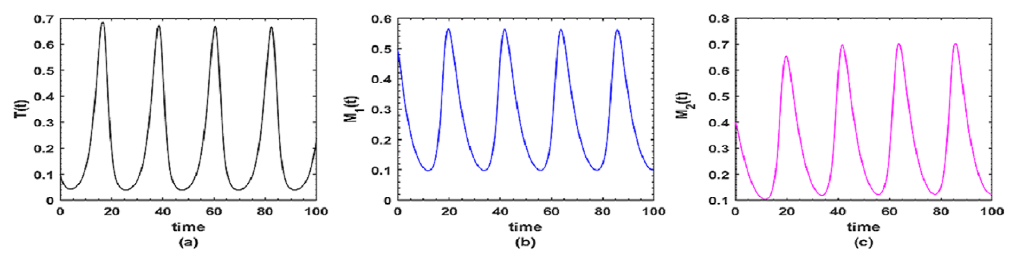
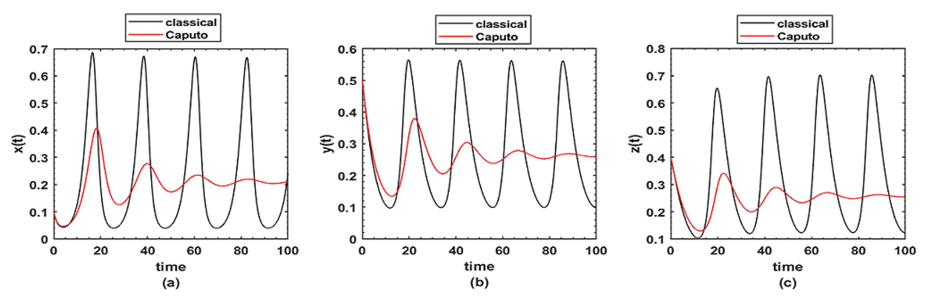
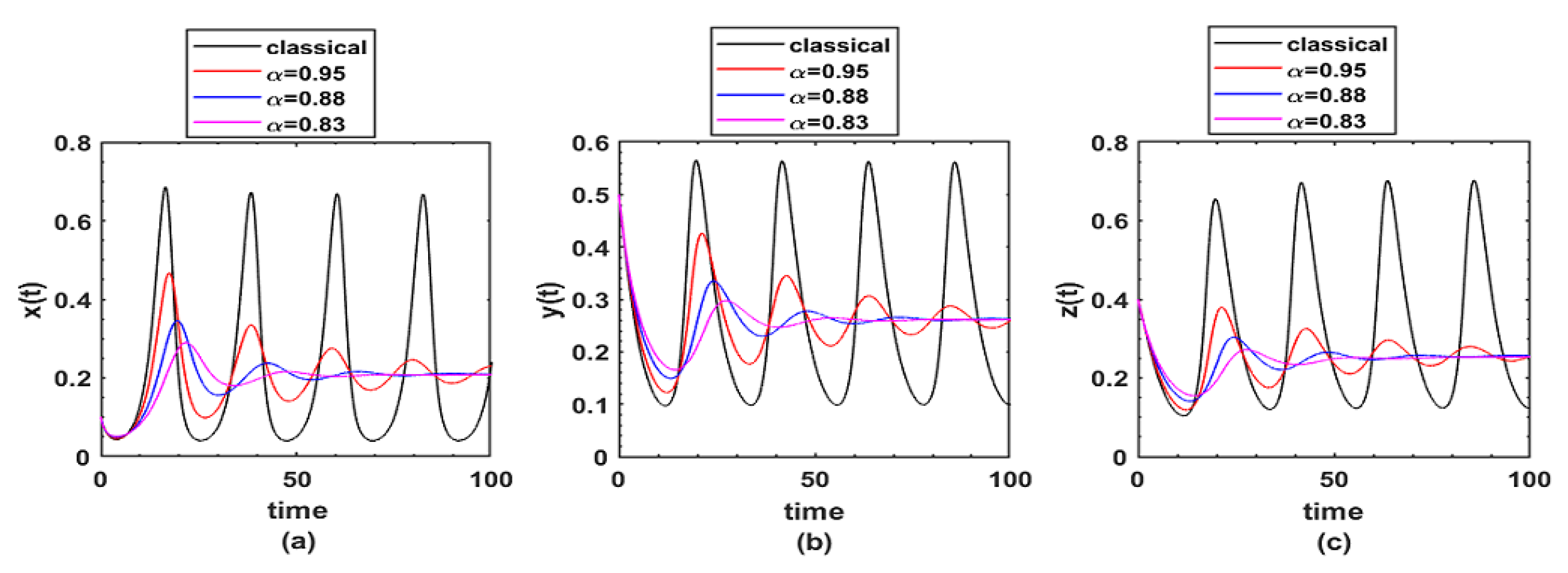
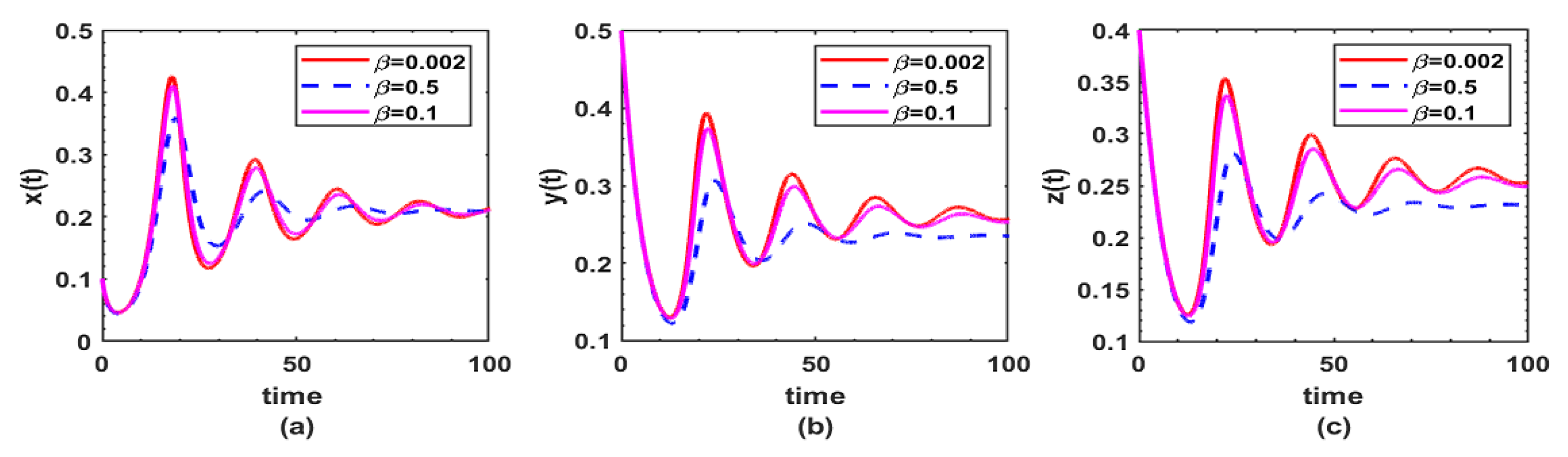
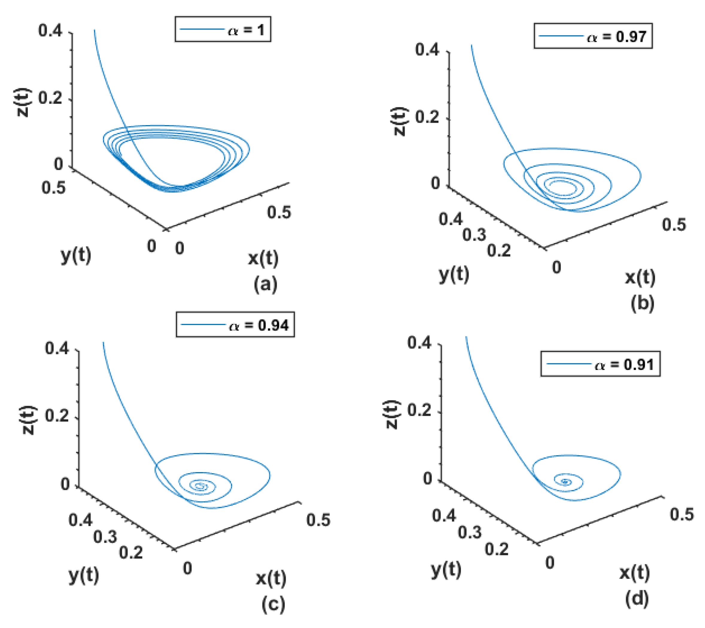
8. Numerical Simulation and Discussion

In order to carry out the numerical simulation of system (2), we will use the predictor–corrector method given by Adams–Bashforth–Moulton. To obtain the approximate solution of system (2) by using this method, we consider the following system of nonlinear fractional differential Equation [46]:

$$\begin{array}{c}\hfill D_t^{\alpha }\psi \left(t\right)=F(t,\psi \left(t\right)),0\le t\le T,{\psi }^m\left(0\right)={\psi }_0^m,m=0,1,2,\dots ,k-1,\end{array}$$

(12)

where $\alpha >0$ and $k=\lceil \alpha \rceil$ is the integer greater than or equal to $\alpha$. The $\alpha th$ order fractional derivative of $\psi \left(t\right)$ in Caputo sense denoted by $D_t^{\alpha }\psi \left(t\right)$ is defined by the following:

$$\begin{array}{c}\hfill D_t^{\alpha }f\left(t\right)={\displaystyle \frac{1}{\mathsf{\Gamma }(n-\alpha )}}{\int }_0^t{(t-r)}^{n-\alpha -1}{f}^{\left(n\right)}\left(r\right)dr,n-1<\alpha <n,n\in Z^{+},\end{array}$$

where $f^{\left(n\right)}\left(r\right)$ denotes the $nth$ integer order derivative of $f\left(r\right)$.

The fractional differential Equation (12) is also equivalent to Volterra integral equation given by the following:

$$\begin{array}{c}\hfill \psi \left(t\right)=\sum _{m=0}^{n-1}{\psi }_0^m{\displaystyle \frac{t^m}{m!}}+{\displaystyle \frac{1}{\mathsf{\Gamma }\left(\alpha \right)}}{\int }_0^t{(t-r)}^{\alpha -1}F(r,\psi \left(r\right))dr.\end{array}$$

(13)

The predictor–corrector method of Adams–Bashforth–Moulton is already used in [47,48,49] for integrating Equation (13). The same scheme is applied to our proposed fractional-order model (2) by setting the following: $j={\displaystyle \frac{T}{N}}$, $t_i=ij$, $i=0,1,2,\dots$, $N\in Z^{+}.$

Therefore, fractional-order model (2) can be discretized as follows:

$$\begin{array}{c}\hfill \begin{array}{cc}\hfill x_{n+1}& =x_0+{\displaystyle \frac{j^{\alpha }}{\mathsf{\Gamma }(\alpha +2)}}[[{\varrho }^{{}^{\prime }}{x}_{n+1}^q(1-{\beta }^{{}^{\prime }}{x}_{n+1}^q)-{\delta }^{{}^{\prime }}{x}_{n+1}^q{y}_{n+1}^q+{\eta }^{{}^{\prime }}{x}_{n+1}^q{z}_{n+1}^q]\hfill \\ & +\sum _{i=0}^n{a}_{i,n+1}^{{}^{\prime }}[{\varrho }^{{}^{\prime }}{x}_i(1-{\beta }^{{}^{\prime }}{x}_i)-{\delta }^{{}^{\prime }}{x}_i{y}_i+{\eta }^{{}^{\prime }}{x}_i{z}_i]],\hfill \\ \hfill y_{n+1}& =y_0+{\displaystyle \frac{j^{\alpha }}{\mathsf{\Gamma }(\alpha +2)}}[[x_{n+1}^q{y}_{n+1}^q-{\mu }_1^{{}^{\prime }}{y}_{n+1}^q-{\gamma }_1^{{}^{\prime }}{y}_{n+1}^q+{\gamma }_2^{{}^{\prime }}{z}_{n+1}^q]\hfill \\ & +\sum _{i=0}^n{a}_{i,n+1}^{{}^{\prime }}[x_i{y}_i-{\mu }_1^{{}^{\prime }}{y}_i-{\gamma }_1^{{}^{\prime }}{y}_i+{\gamma }_2^{{}^{\prime }}{z}_i]],\hfill \\ \hfill z_{n+1}& =z_0+{\displaystyle \frac{j^{\alpha }}{\mathsf{\Gamma }(\alpha +2)}}[[{\zeta }^{{}^{\prime }}{x}_{n+1}^q{z}_{n+1}^q-{\mu }_2^{{}^{\prime }}{z}_{n+1}^q+{\gamma }_1^{{}^{\prime }}{y}_{n+1}^q-{\gamma }_2^{{}^{\prime }}{z}_{n+1}^q]\hfill \\ & +\sum _{i=0}^n{a}_{i,n+1}^{{}^{\prime }}[{\zeta }^{{}^{\prime }}{x}_i{y}_i-{\mu }_2^{{}^{\prime }}{z}_i+{\gamma }_1^{{}^{\prime }}{y}_i-{\gamma }_2^{{}^{\prime }}{z}_i]],\hfill \end{array}\end{array}$$

(14)

where,

$$\begin{array}{c}\hfill \begin{array}{cc}\hfill x_{n+1}^q& =x_0+{\displaystyle \frac{1}{\mathsf{\Gamma }\left(\alpha \right)}}\sum _{p=0}^n{b}_{p,n+1}^{{}^{\prime }}[{\varrho }^{{}^{\prime }}{x}_p(1-{\beta }^{{}^{\prime }}{x}_p)-{\delta }^{{}^{\prime }}{x}_p{y}_p+{\eta }^{{}^{\prime }}{x}_p{z}_p],\hfill \\ \hfill y_{n+1}^q& =y_0+{\displaystyle \frac{1}{\mathsf{\Gamma }\left(\alpha \right)}}\sum _{p=0}^n{b}_{p,n+1}^{{}^{\prime }}[x_p{y}_p-{\mu }_1^{{}^{\prime }}{y}_p-{\gamma }_1^{{}^{\prime }}{y}_p+{\gamma }_2^{{}^{\prime }}{z}_p],\hfill \\ \hfill z_{n+1}^q& =z_0+{\displaystyle \frac{1}{\mathsf{\Gamma }\left(\alpha \right)}}\sum _{p=0}^n{b}_{p,n+1}^{{}^{\prime }}[{\zeta }^{{}^{\prime }}{x}_p{y}_p-{\mu }_2^{{}^{\prime }}{z}_p+{\gamma }_1^{{}^{\prime }}{y}_p-{\gamma }_2^{{}^{\prime }}{z}_p].\hfill \end{array}\end{array}$$

(15)

For different ranges of values of i, we will obtain the following four different results for $a_{i,n+1}^{{}^{\prime }}$:

$$\begin{array}{c}\hfill a_{i,n+1}^{{}^{\prime }}={\displaystyle \frac{j^{\alpha }}{\alpha (\alpha +1)}}\left\{\begin{array}{cc}\left(n^{\alpha +1}-(n-\alpha ){(n+1)}^{\alpha }\right),\hfill & ifi=0\hfill \\ \left({(n-i+2)}^{\alpha +1}+{(n-i)}^{\alpha +1}-2{(n-i+1)}^{\alpha +1}\right),\hfill & if1\le i\le n\hfill \\ 1,\hfill & ifi=n+1\hfill \end{array}\right..\end{array}$$

(16)

Similarly, $b_{p,n+1}^{{}^{\prime }}$ can be obtained by using the following result:

$$\begin{array}{c}\hfill b_{p,n+1}^{{}^{\prime }}={\displaystyle \frac{j^{\alpha }}{\alpha }}[{(n+1-i)}^{\alpha }-{(n-i)}^{\alpha }].\end{array}$$

(17)

For numerical simulation and graphical analysis of the generalized model (2), we choose the numerical values of the parameters and variables from Table 1. Most of the numerical simulations are performed with the help of MATLAB software.

After using the above-discussed numerical scheme, the proposed model is simulated while using the biological parameters considered in the present research paper. We have presented not only time series plots but also included the three-dimensional behavior of the system for a clear understanding of the disease transmission. Some important biological parameters are chosen to observe their effects on the state variables of the system. The system is simulated while considering the Caputo version, as discussed in earlier sections. Several values of the fractional order $\alpha$ are taken to check the performance of the proposed model.

As a matter of necessity, fractional operators are included in several types of diffusion issues. There is just a rough association between relaxation kernels and the fractional orders they entail (for example, the correlation function). The Caputo fractional-order operator can be used to provide a mathematical description of the dynamics of systems exhibiting memory effects or long-term persistence. Within the context of an epidemiological model, it can be used to describe the dispersal of a disease within a community. Attractors can be thought of as the steady state or equilibrium towards which a model epidemic system tends to converge over time. The dynamics of the system can be described by the Caputo fractional-order operator, and the attractor can be thought of as the long-term consequence of those dynamics in an epidemiological model. The cycles that exist as solutions (asymptotically fixed points) of the system here vanish when the patient either fully recovers following treatment or vaccination or passes away, and this is quite often seen in real medical cases.

First, we plotted each equation of model (1) separately to have a look at the population growth of tumor cells, $M_1$ cells, and $M_2$ cells, as shown in Figure 3. Then, we plotted each equation of the fractional-order model (2) separately for different values of fractional-order parameter $\alpha$, as shown in Figure 4. This shows that there are some unexpected fluctuations in the growth curves of the cell populations as the value of $\alpha$ increases. Similarly, Figure 5 represents the comparison between the growth curves of the cell populations in models (1) and (2) with respect to time t. Here, we choose $\alpha =0.92$. Furthermore, Figure 6 shows the fluctuations in the growth curves of three cell populations in both models while choosing the values of parameter $\alpha$ as $0.95$, $0.88$, and $0.83$.

As observed in Figure 7 with the fractional order $\alpha =0.93$, the oscillatory phenomenon is encountered for each state variable of the model. Nonetheless, the oscillatory behavior decreases its amplitude once the value of $\beta$ increases. Similarly, the population of tumor cells $x\left(t\right)$ increases with an increasing value of $\delta$ while the rest of the two populations decrease with increasing $\delta$ when the fractional order is taken to be 0.93, as shown in Figure 8.

As can be seen in Figure 9 and Figure 10, the three-dimensional plots depict clearly what is happening before taking into consideration the classical time derivative ($\alpha =1$). Looking at the spirals in said figures, the periodic behavior is confirmed, as shown by the time series plots in two dimensions. With increasing values of $\alpha$, the memory of the disease is evident, as we can clearly see how the periodic pattern is formed. For Figure 10, we not only varied $\alpha$ but also taken into consideration the $\zeta$ to know its effects on the surfaces obtained for the three state variables of the proposed model. The entire memory of the disease is captured during the simulations since we can see how the spiral behavior is formed with increasing values of the fractional order $\alpha$.

9. Concluding Remarks with Future Prospects

The focus of this study is on applying the Caputo fractional-order differential operator to the construction of a nonlinear system of ordinary differential equations in three dimensions. The suggested system illustrates the dynamics of the spread of a disease manifested in the interactions between tumors and macrophages. It demonstrates how the lineage of memory may be tracked back through time. Existence, uniqueness, and stability analysis have all been well examined; therefore, the model’s qualitative analysis is solid. One of the main contributions of this work is the optimization of the fractional order $\alpha$ to be 7.156 × ${10}^{-1}$ using real-world incidence cases of the tumor cells from 15 September to 28 September 2022. Several graphs illustrating the impact of various biological parameters on the disease transmission dynamics were included in the numerical simulations to provide further confirmation of the theoretical study. Since most infectious diseases have memories due to reemergence in the community, it is concluded that the Caputo operator is among the best choices to be utilized for simulating infectious diseases since its hereditary properties fit with the behavior of the disease. Future research will focus on fractional-order operators, such as the Atangana–Baleanu operator, the Caputo–Fabrizio operator, and the proportional one. For example, these operators will be used to estimate biological parameters, which will be based on real medical data.

References

1. Niu, H.; Chen, Y.; West, B.J. Why Do Big Data and Machine Learning Entail the Fractional Dynamics? Entropy 2021, 23, 297. [Google Scholar] [CrossRef] [PubMed]
2. Dunn, G.P.; Old, L.J.; Schreiber, R.D. The three Es of cancer immunoediting. Annu. Rev. Immunol. 2004, 22, 329–360. [Google Scholar] [CrossRef] [PubMed]
3. Mantovani, A.; Sozzani, S.; Locati, M.; Allavena, P.; Sica, A. Macrophage polarization: Tumor-associated macrophages as a paradigm for polarized M2 mononuclear phagocytes. Trends. Immunol. 2002, 23, 549–555. [Google Scholar] [CrossRef] [PubMed]
4. Sica, A.; Larghi, P.; Mancino, A.; Rubino, L.; Porta, C.; Totaro, M.G.; Rimoldi, M.; Biswas, S.K.; Allavena, P.; Mantovani, A. Macrophage polarization in tumor progression. Semin. Cancer Biol. 2008, 18, 349–355. [Google Scholar] [CrossRef] [PubMed]
5. Yaqin, S.; Jicai, H.; Yueping, D.; Yasuhiro, T. Mathematical modelling and bifurcation analysis of pro and anti-tumor macrophages. APM 2020, 2020, 13468. [Google Scholar]
6. Allavena, P.; Mantovani, A. Immunology in the clinic review series; focus on cancer: Tumor-associated macrophages: Undisputed stars of the inflammatory tumor microenvironment. Clin. Exp. Immunol. 2012, 167, 195–205. [Google Scholar] [CrossRef]
7. Anderson, L.; Jang, S.; Yu, J.L. Qualitative behavior of systems of CD4+ cytokine interactions with treatments. Math. Method Appl. Sci. 2015, 38, 4330–4344. [Google Scholar] [CrossRef]
8. Saadeh, R.; Qazza, A.; Amawi, K. A New Approach Using Integral Transform to Solve Cancer Models. Fractal Fract. 2022, 6, 490. [Google Scholar] [CrossRef]
9. Kuznetsov, V.A.; Makalkin, I.A.; Taylor, M.A.; Perelson, S. Nonlinear dynamics of immunogenic tumors: Parameter estimation and global bifurcation analysis. Bull. Math. Biol. 1994, 56, 295–321. [Google Scholar] [CrossRef]
10. Kuznetsov, V.A.; Knott, G.D. modelling tumor regrowth and immunotherapy. Math. Comput. Modell. 2001, 33, 1275–1287. [Google Scholar] [CrossRef] [Green Version]
11. Levy, J.A. The importance of the innate immune system in controlling HIV infection and disease. Trends Immunol. 2001, 22, 312–316. [Google Scholar] [CrossRef]
12. Banerjee, S.; Sarkar, R.R. Delay-induced model for tumor–immune interaction and control of malignant tumor growth. Biosystems 2008, 91, 268–288. [Google Scholar] [CrossRef]
13. Pang, L.; Liu, S.; Liu, F.; Zhang, X.; Tian, T. Mathematical modeling and analysis of tumor-volume variation during radiotherapy. Appl. Math. Model. 2021, 89, 1074–1089. [Google Scholar] [CrossRef]
14. Duan, W.L.; Fang, H.; Zeng, C. The stability analysis of tumor-immune responses to chemotherapy system with gaussian white noises. Chaos Solitons Fractals 2019, 127, 96–102. [Google Scholar] [CrossRef]
15. Eftimie, R.; Barelle, C. Mathematical investigation of innate immune responses to lung cancer: The role of macrophages with mixed phenotypes. J. Theor. Biol. 2021, 524, 110739. [Google Scholar] [CrossRef]
16. Sarmah, D.T.; Bairagi, N.; Chatterjee, S. The interplay between DNA damage and autophagy in lung cancer: A mathematical study. Biosystems 2021, 206, 104443. [Google Scholar] [CrossRef]
17. Dong, Y.; Huang, G.; Miyazaki, R.; Takeuchi, Y. Dynamics in a tumor immune system with time delays. Appl. Math. Comput. 2015, 252, 99–113. [Google Scholar] [CrossRef]
18. Villasana, M.; Radunskaya, A. A delay differential equation model for tumor growth. J. Math. Biol. 2003, 47, 270–294. [Google Scholar] [CrossRef]
19. Gałach, M. Dynamics of the tumor-immune system competition—The effect of time delay. Int. J. Appl. Math. Comput. Sci. 2003, 13, 395–406. [Google Scholar]
20. Shen, W.Y.; Chu, Y.M.; ur Rahman, M.; Mahariq, I.; Zeb, A. Mathematical analysis of HBV and HCV co-infection model under nonsingular fractional order derivative. Results Phys. 2021, 28, 104582. [Google Scholar] [CrossRef]
21. Chu, Y.M.; Khan, M.F.; Ullah, S.; Shah, S.A.A.; Farooq, M.; bin Mamat, M. Mathematical assessment of a fractional-order vector–host disease model with the Caputo–Fabrizio derivative. Math. Methods Appl. Sci. 2023, 46, 232–247. [Google Scholar] [CrossRef]
22. Li, P.; Gao, R.; Xu, C.; Li, Y.; Akgül, A.; Baleanu, D. Dynamics exploration for a fractional-order delayed zooplankton–phytoplankton system. Chaos Solitons Fractals 2023, 166, 112975. [Google Scholar] [CrossRef]
23. Ding, Y.; Wang, Z.; Ye, H. Optimal control of a fractional-order HIV-immune system with memory. IEEE Trans. Control Syst. Technol. 2012, 20, 763–769. [Google Scholar] [CrossRef]
24. Bolton, L.; Cloot, A.H.; Schoombie, S.W.; Slabbert, J.P. A proposed fractional-order gompertz model and its application to tumor growth data. Math. Med. Biol. 2015, 32, 187–207. [Google Scholar] [CrossRef] [PubMed]
25. Ahmed, E.; Hashish, A.; Rihan, F.A. On fractional order cancer model. J. Fract. Calc. Appl. Anal. 2012, 3, 1–6. [Google Scholar]
26. Rihan, F.A.; Hashish, A.; Al-Maskari, F.; Hussein, M.S.; Ahmed, E.; Riaz, M.B.; Yafia, R. Dynamics of tumor-immune system with fractional-order. J. Tumor Res. 2016, 2, 109. [Google Scholar] [CrossRef]
27. Tuan, N.H.; Mohammadi, H.; Rezapour, S. A mathematical model for COVID-19 transmission by using the Caputo fractional derivative. Chaos Solitons Fractals 2020, 140, 110107. [Google Scholar] [CrossRef]
28. Ali, A.; Alshammari, F.S.; Islam, S.; Khan, M.A.; Ullah, S. Modeling and analysis of the dynamics of novel coronavirus (COVID-19) with Caputo fractional derivative. Results Phys. 2021, 20, 103669. [Google Scholar] [CrossRef]
29. Nisar, K.S.; Ahmad, S.; Ullah, A.; Shah, K.; Alrabaiah, H.; Arfan, M. Mathematical analysis of SIRD model of COVID-19 with Caputo fractional derivative based on real data. Results Phys. 2021, 21, 103772. [Google Scholar] [CrossRef]
30. Ahmed, I.; Baba, I.A.; Yusuf, A.; Kumam, P.; Kumam, W. Analysis of Caputo fractional-order model for COVID-19 with lockdown. Adv. Differ. Equ. 2020, 2020, 394. [Google Scholar] [CrossRef]
31. Yadav, R.P.; Verma, R. A numerical simulation of fractional order mathematical modeling of COVID-19 disease in case of Wuhan China. Chaos Solitons Fractals 2020, 140, 110124. [Google Scholar] [CrossRef]
32. Mohammad, M.; Trounev, A.; Cattani, C. The dynamics of COVID-19 in the UAE based on fractional derivative modeling using Riesz wavelets simulation. Adv. Differ. Equ. 2021, 2021, 115. [Google Scholar] [CrossRef]
33. Owen, M.R.; Sherratt, J.A. Modelling the macrophage invasion of tumors: Effects on growth and composition. IMA J. Math. Appl. Med. Biol. 1998, 15, 165–185. [Google Scholar] [CrossRef]
34. El-Sayed, A.M.A.; El-Mesiry, A.E.M.; El-Saka, H.A.A. On the fractional- order logistic equation. Appl. Math. Lett. 2007, 20, 817–823. [Google Scholar] [CrossRef] [Green Version]
35. Petras, I. Fractional-Order Nonlinear Systems: Modeling, Analysis and Simulation; Springer: Berlin, Germany, 2011. [Google Scholar]
36. Baisad, K.; Moonchai, S. Analysis of stability and hopf bifurcation in a fractional gauss-type predator-prey model with allee effect and holling type-III functional response. Adv. Diff. Equ. 2018, 2018, 82. [Google Scholar] [CrossRef] [Green Version]
37. Ahmed, E.; El-Sayed, A.M.A.; El-Saka, H.A.A. Equilibrium points, stability and numerical solutions of fractional-order predator-prey and rabies models. J. Math. Anal. Appl. 2007, 325, 542–553. [Google Scholar] [CrossRef] [Green Version]
38. Bozkurt, F.; Abdeljawad, T.; Hajji, M.A. Stability analysis of a fractional-order differential equation model of a brain tumor growth depending on the density. Appl. Comput. Math. 2015, 14, 50–62. [Google Scholar]
39. Öztürk, I.; Özköse, F. Stability analysis of fractional order mathematical model of tumor-immune system interaction. Chaos Solitons Fractals 2020, 133, 109614. [Google Scholar] [CrossRef]
40. Özköse, F.; Yılmaz, S.; Yavuz, M.; Öztürk, İ.; Şenel, M.T.; Bağcı, B.Ş.; Doğan, M.; Önal, Ö. A fractional modeling of tumor–immune system interaction related to Lung cancer with real data. Eur. Phys. J. Plus 2022, 137, 40. [Google Scholar] [CrossRef]
41. Solit, D.B.; Garraway, L.A.; Pratilas, C.A.; Sawai, A.; Getz, G.; Basso, A.; Ye, Q.; Lobo, J.M.; She, Y.; Osman, I.; et al. BRAF mutation predicts sensitivity to MEK inhibition. Nature 2006, 439, 358–362. [Google Scholar] [CrossRef] [Green Version]
42. da Hora, C.C.; Wurdinger, M.W.S.T.; Tannous, B.A. Patient-derived glioma models: From patients to dish to animals. Cells 2019, 8, 1177. [Google Scholar] [CrossRef] [PubMed] [Green Version]
43. Burdall, S.E.; Hanby, A.M.; Lansdown, M.R.; Speirs, V. Breast cancer cell lines: Friend or foe? Breast Cancer Res. 2003, 5, 89. [Google Scholar] [CrossRef] [PubMed] [Green Version]
44. Matignon, D. Stability results for fractional differential equations with applications to control processing. Comput. Eng. Syst. Appl. 1996, 2, 963. [Google Scholar]
45. Mishina, A.P.; Proskuryakov, I.V. Higher Algebra; Nauka: Moscow, Russia, 1965. [Google Scholar]
46. Li, C.; Tao, C. On the fractional adams method. Comput. Math. Appl. 2009, 58, 1573–1588. [Google Scholar] [CrossRef] [Green Version]
47. Diethelm, K. An algorithm for the numerical solution of differential equations of fractional order. Electron. Trans. Numer. Anal. 1997, 5, 1–6. [Google Scholar]
48. Diethelm, K.; Ford, N.J.; Freed, A.D. A predictor-corrector approch for the numerical solution of fractional differential equations. Nonlinear Dyn. 2002, 29, 3–22. [Google Scholar] [CrossRef]
49. Diethelm, K.; Ford, N.J. Analysis of fractional differential equations. J. Math. Anal. Appl. 2002, 265, 229–248. [Google Scholar] [CrossRef] [Green Version]
Figure 1. Comparison of real medical data of tumor cells with the best-fitted curves of (a) classical model given in (1) and (b) Caputo model given in (2).
Fractalfract 07 00258 g001
Figure 2. The Box and Whisker plot for the statistical comparison among real medical data and simulations obtained with classical and Caputo versions of the model for the number of tumor cells.
Fractalfract 07 00258 g002
Figure 3. The dynamical behavior of three state variables in the classical model (1) over the time interval [ 0 , 100 ] , while biological parameters are taken from Table 1 with time unit in days.
Fractalfract 07 00258 g003
Figure 4. The dynamical behavior of three state variables in the Caputo fractional-order model 2 under different values of the fractional order α over the time interval [ 0 , 100 ] , while biological parameters are taken from Table 1 with time unit in days.
Fractalfract 07 00258 g004
Figure 5. The dynamical behavior of three state variables in both classical and the Caputo fractional mode while taking α = 0.92 for the latter over the time interval [ 0 , 100 ] , while biological parameters are taken from Table 1 with time unit in days.
Fractalfract 07 00258 g005
Figure 6. The dynamical behavior of three state variables in both classical and the Caputo fractional mode over the time interval [ 0 , 100 ] , while biological parameters are taken from Table 1 with time unit in days.
Fractalfract 07 00258 g006
Figure 7. The dynamical behavior of three state variables in the Caputo model with α = 0.93 over the time interval [ 0 , 100 ] , while biological parameters are taken from Table 1 with time unit in days.
Fractalfract 07 00258 g007
Figure 8. The dynamical behavior of three state variables in the Caputo model with α = 0.93 over the time interval [ 0 , 100 ] , while biological parameters are taken from Table 1 with time unit in days.
Fractalfract 07 00258 g008
Figure 9. The dynamical behavior of three state variables with different values of α .
Fractalfract 07 00258 g009
Figure 10. The dynamical behavior of three state variables with different values of α while ζ = 9 × 10 7 .
Fractalfract 07 00258 g010