
Solitary Wave Solutions to a Fractional Model Using the Improved Modified Extended Tanh-Function Method

Abstract
:1. Introduction
2. The Jumarie’s Modified Riemann–Liouville Derivative
3. Improved Modified Extended Tanh-Function Technique
4. Traveling Wave Solutions of SRLW Equation
- First family of solutions
- Second family of solutions
- Third family of solutions
- Fourth family of solutions
- Fifth family of solutions
- Sixth family of solutions
5. Result and Discussion
6. Conclusions
Funding
Data Availability Statement
Conflicts of Interest
Appendix A
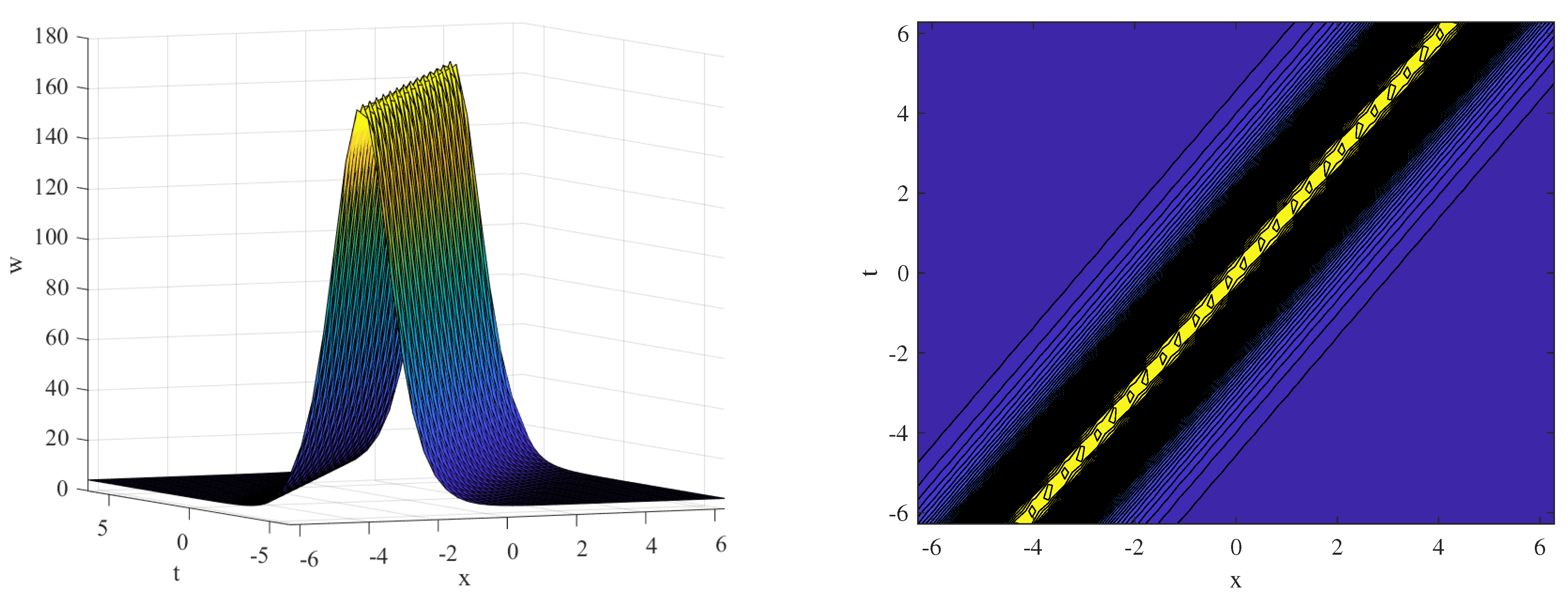
- First case: If , then a bell-shaped solitary wave solution, a triangular type solution, and a rational solution for Equation (6) are shown as follows:
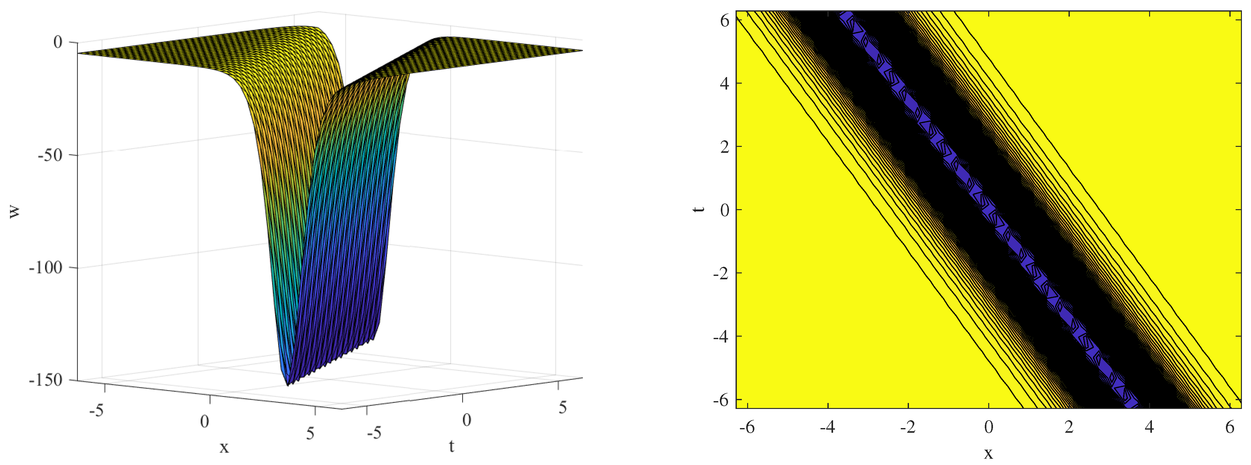
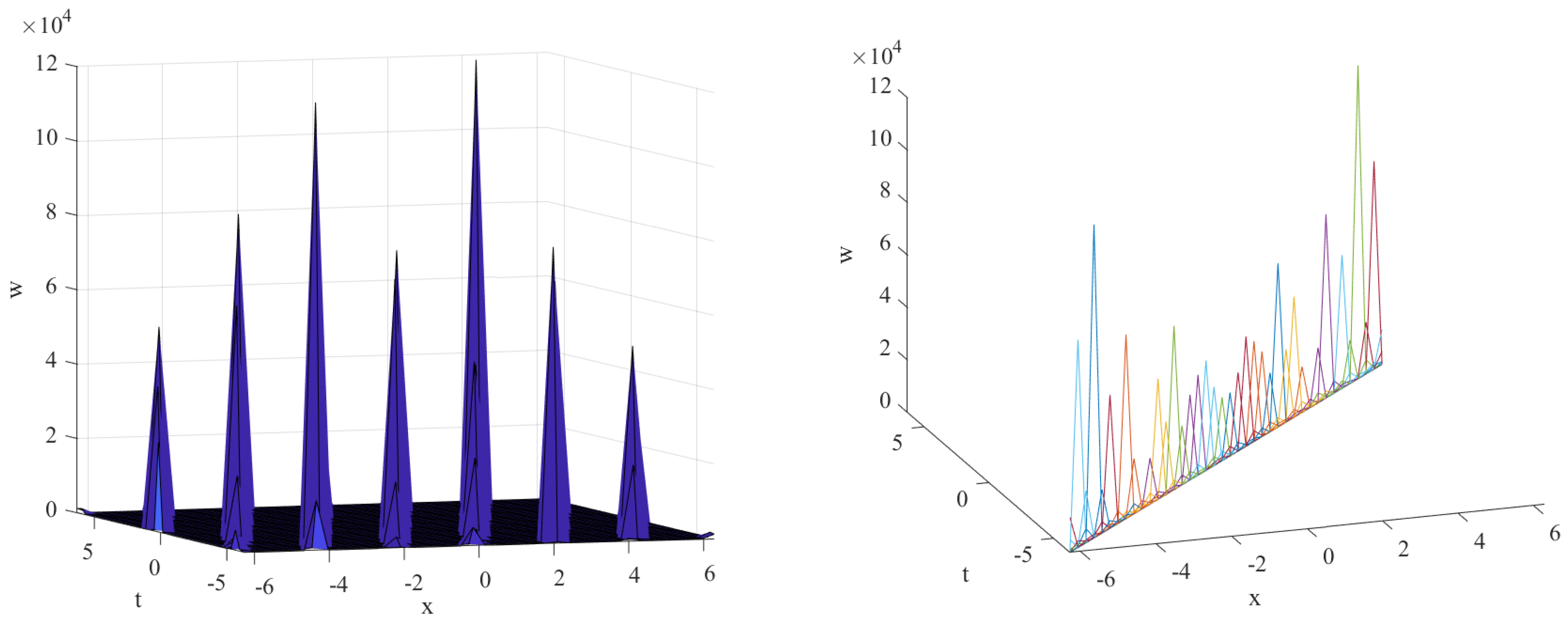
- Second case: If , then a kink-shaped solitary wave solution, a triangular type solution, and three Jacobi elliptic doubly periodic type solutions for Equation (6) are given as follows:where m denotes a modulus.
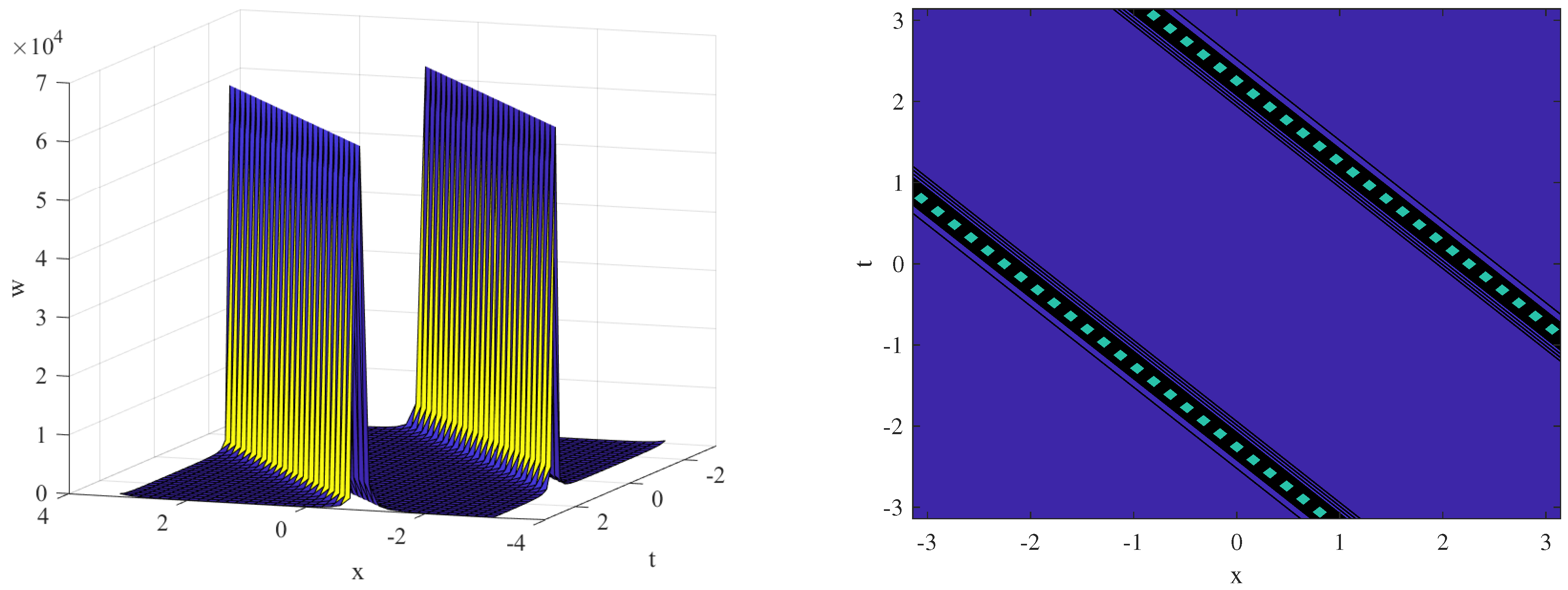
- Third case: If , then a bell-shaped solitary wave solution, a triangular type solution, and a rational solution for Equation (6) are given by
References
- Al-Amin, M.; Nurul Islam, M.; Ali Akbar, M. Abundant Exact Soliton Solutions to the Space-Time Fractional Phi-Four Effective Model for Quantum Effects Through the Modern Scheme. Int. J. Sci. Basic Appl. Res. 2021, 60, 1–16. [Google Scholar]
- Wang, M.J.; Wang, Q. Application of rational expansion method for stochastic differential equations. Appl. Math. Comput. 2012, 218, 5259–5264. [Google Scholar] [CrossRef]
- Syam Kumar, A.M.; Prasanth, J.P.; Bannur, V.M. Quark-gluon plasma phase transition using cluster expansion method. Phys. A Stat. Mech. Its Appl. 2015, 432, 71–75. [Google Scholar] [CrossRef]
- He, J.H. Homotopy perturbation method for bifurcation of nonlinear problems. Int. J. Nonlinear Sci. Numer. Simul. 2005, 6, 207–208. [Google Scholar] [CrossRef]
- Esen, A. A numerical solution of the equal width wave equation by a lumped Galerkin method. Appl. Math. Comput. 2005, 168, 270–282. [Google Scholar] [CrossRef]
- Hirota, R. Exact N-soliton solutions of the wave equation of long waves in shallow water and in nonlinear lattices. JMP 1973, 14, 810–814. [Google Scholar] [CrossRef]
- Wang, M.; Li, X.; Zhang, J. The ()-expansion method and travelling wave solutions of nonlinear evolution equations in mathematical physics. Phys. Lett. A 2008, 372, 417–423. [Google Scholar] [CrossRef]
- Aasaraai, A. The Application of Modified F-expansion Method Solving the Maccari’s System. J. Adv. Math. Comput. Sci. 2015, 11, 1–14. [Google Scholar] [CrossRef]
- Alharbi, A.R.; Almatrafi, M.B. Numerical investigation of the dispersive long wave equation using an adaptive moving mesh method and its stability. Results Phys. 2020, 16, 102870. [Google Scholar] [CrossRef]
- Almatrafi, M.B.; Alharbi, A.R.; Tunç, C. Constructions of the soliton solutions to the good Boussinesq equation. Adv. Differ. Equ. 2020, 629, 142–149. [Google Scholar] [CrossRef]
- Zhu, W.; Ling, Z.; Xia, Y.; Gao, M. Bifurcations and the Exact Solutions of the Time-Space Fractional Complex Ginzburg-Landau Equation with Parabolic Law Nonlinearity. Fractal Fract. 2023, 7, 201. [Google Scholar] [CrossRef]
- Wu, G.; Guo, Y. New Complex Wave Solutions and Diverse Wave Structures of the (2+1)-Dimensional Asymmetric Nizhnik–Novikov–Veselov Equation. Fractal Fract. 2023, 7, 170. [Google Scholar] [CrossRef]
- Ur Rahman, R.; Faridi, W.A.; El-Rahman, M.A.; Taishiyeva, A.; Myrzakulov, R.; Az-Zo’bi, E.A. The Sensitive Visualization and Generalized Fractional Solitons’ Construction for Regularized Long-Wave Governing Model. Fractal Fract. 2023, 7, 136. [Google Scholar] [CrossRef]
- Almatrafi, M.B. Abundant traveling wave and numerical solutions for Novikov-Veselov system with their stability and accuracy. Appl. Anal. 2022, 1–14. [Google Scholar] [CrossRef]
- Ross, B. The development of fractional calculus. Hist. Math. 1977, 4, 75–89. [Google Scholar] [CrossRef]
- Miller, K.S.; Ross, B. An Introduction to the Fractional Calculus and Fractional Differential Equations; John Wiley & Sons: New York, NY, USA, 1993. [Google Scholar]
- Riemann, B. Versuch Einer Allgemeinen Auffassung der Integration und Differentiation. In Gesammelte Mathematische Werke und Wissenschaftlicher Nachlass; Teubner: Leipzig, Germany; Dover: New York, NY, USA, 1953. [Google Scholar]
- Oliveira, E.C.D.; Machado, J.A.T. Machado, A Review of Definitions for Fractional Derivatives and Integral. Math. Probl. Eng. 2014, 2014, 238459. [Google Scholar] [CrossRef]
- Seyler, C.E.; Fenstermacher, D.L. A symmetric regularized-long-wave equation. Phys. Fluids 1984, 27, 4–7. [Google Scholar] [CrossRef]
- Xu, F. Application of Exp-function method to Symmetric Regularized Long Wave (SRLW) equation. Phys. Lett. A 2008, 372, 252–257. [Google Scholar] [CrossRef]
- Alzaidy, J.F. The fractional sub-equation method and exact analytical solutions for some nonlinear fractional PDEs. Am. J. Math. Anal. 2013, 1, 14–19. [Google Scholar]
- Shakeel, M.; Mohyud-Din, S.T. A novel G′/G-expansion method and its application to the space-time fractional symmetric regularized long wave (SRLW) equation. Adv. Trends Math. 2015, 2, 1–16. [Google Scholar] [CrossRef]
- Yaro, D.; Seadawy, A.R.; Lu, D.; Apeanti, W.O.; Akuamoah, S.W. Dispersive wave solutions of the nonlinear fractional Zakhorov-Kuznetsov- Benjamin-Bona-Mahony equation and fractional symmetric regularized long wave equation. Results Phys. 2019, 12, 1971–1979. [Google Scholar] [CrossRef]
- Khan, M.A.; Akbar, M.A.; Hamid, N. Traveling wave solutions for space-time fractional Cahn Hilliard equation and space-time fractional symmetric regularized long-wave equation. Alex. Eng. J. 2021, 60, 1317–1324. [Google Scholar] [CrossRef]
- Ünal, S.C.; Dascoğlu, A.; Varol, D. Jacobi elliptic function solutions of space-time fractional symmetric regularized long wave equation. Math. Sci. Appl. E-Notes 2021, 9, 53–63. [Google Scholar] [CrossRef]
- Zhu, Q.; Qi, J. Exact solutions of the nonlinear space-time fractional partial differential symmetric regularized long wave (SRLW) equation by employing two methods. Adv. Math. Phys. 2022, 2022, 8062119. [Google Scholar] [CrossRef]
- Yang, Z.; Hon, B.Y.C. An Improved Modified Extended tanh-Function Method. Z. Naturforschung A 2006, 61, 103–115. [Google Scholar] [CrossRef]
- Khalil, R.; Horani, M.A.; Yousef, A.; Sababheh, M. A new definition of fractional derivative. J. Comput. Appl. Math. 2014, 264, 65–70. [Google Scholar] [CrossRef]
- Jumarie, G. Modified Riemann-Liouville derivative and fractional Taylor series of nondifferentiable functions further results. Comput. Math. Appl. 2006, 51, 1367–1376. [Google Scholar] [CrossRef]
- Li, Q.; Soybaş, D.; Ilhan, O.A.; Singh, G.; Manafian, J. Pure Traveling Wave Solutions for Three Nonlinear Fractional Models. Adv. Math. Phys. 2021, 2021, 6680874. [Google Scholar]
- Ala, V.; Demirbilek, U.; Mamedov, K.R. An application of improved Bernoulli sub-equation function method to the nonlinear conformable time-fractional SRLW equation. Aims Math. 2020, 5, 3751–3761. [Google Scholar] [CrossRef]
- Sonmezoglu, A. Exact solutions for some fractional differential equations. Adv. Math. Phys. 2015, 2015, 567842. [Google Scholar] [CrossRef]


Disclaimer/Publisher’s Note: The statements, opinions and data contained in all publications are solely those of the individual author(s) and contributor(s) and not of MDPI and/or the editor(s). MDPI and/or the editor(s) disclaim responsibility for any injury to people or property resulting from any ideas, methods, instructions or products referred to in the content. |
© 2023 by the author. Licensee MDPI, Basel, Switzerland. This article is an open access article distributed under the terms and conditions of the Creative Commons Attribution (CC BY) license (https://creativecommons.org/licenses/by/4.0/).
Share and Cite
Almatrafi, M.B. Solitary Wave Solutions to a Fractional Model Using the Improved Modified Extended Tanh-Function Method. Fractal Fract. 2023, 7, 252. https://doi.org/10.3390/fractalfract7030252
Almatrafi MB. Solitary Wave Solutions to a Fractional Model Using the Improved Modified Extended Tanh-Function Method. Fractal and Fractional. 2023; 7(3):252. https://doi.org/10.3390/fractalfract7030252
Chicago/Turabian StyleAlmatrafi, Mohammed Bakheet. 2023. "Solitary Wave Solutions to a Fractional Model Using the Improved Modified Extended Tanh-Function Method" Fractal and Fractional 7, no. 3: 252. https://doi.org/10.3390/fractalfract7030252