Article

The Propagating Exact Solitary Waves Formation of Generalized Calogero–Bogoyavlenskii–Schiff Equation with Robust Computational Approaches

1
Department of Chemical Engineering, College of Engineering, King Khalid University, Abha 61421, Saudi Arabia
2
Department of Mathematics, University of Management and Technology, Lahore 54770, Pakistan
3
Department of Electrical Energy and Management, Faculty of Electrical Engineering, Technical University of Cluj-Napoca, 400114 Cluj-Napoca, Romania
4
Department of Computer Science and Mathematics, Lebanese American University, Beirut 11022801, Lebanon
5
Department of Mathematics, Art and Science Faculty, Siirt University, Siirt 56100, Turkey
6
Mathematics Research Center, Department of Mathematics, Near East University, Near East Boulevard, Mersin 10, Nicosia 99138, Turkey
7
Applied Mathematical Physics Research Group, Physics Department, Faculty of Science, Mansoura University, Mansoura 35516, Egypt
8
Higher Institute of Engineering and Technology, New Damietta 34517, Egypt
*
Author to whom correspondence should be addressed.
Fractal Fract. 2023, 7(2), 191; https://doi.org/10.3390/fractalfract7020191
Submission received: 9 January 2023 / Revised: 3 February 2023 / Accepted: 7 February 2023 / Published: 14 February 2023

Abstract

:
The generalized Calogero–Bogoyavlenskii–Schiff equation (GCBSE) is examined and analyzed in this paper. It has several applications in plasma physics and soliton theory, where it forecasts the soliton wave propagation profiles. In order to obtain the analytically exact solitons, the model under consideration is a nonlinear partial differential equation that is turned into an ordinary differential equation by using the next traveling wave transformation. The new extended direct algebraic technique and the modified auxiliary equation method are applied to the generalized Calogero–Bogoyavlenskii–Schiff equation to get new solitary wave profiles. As a result, novel and generalized analytical wave solutions are acquired in which singular solutions, mixed singular solutions, mixed complex solitary shock solutions, mixed shock singular solutions, mixed periodic solutions, mixed trigonometric solutions, mixed hyperbolic solutions, and periodic solutions are included with numerous soliton families. The propagation of the acquired soliton solution is graphically presented in contour, two- and three-dimensional visualization by selecting appropriate parametric values. It is graphically demonstrated how wave number impacts the obtained traveling wave structures.

1. Introduction

Recently, applications of nonlinear evolution equations (NLEEs) have been showing their imperative rules in physical science, applied science, and design, beginning not long ago with a widespread interest among various scientists, specialists, and researchers. Evolution equations can be used to predict the path of a number of physical problems or complex issues. Due to these abilities, optics, dense-matter physical science, astronomy, biomechanics, high-energy material science, electrical design, synthetic kinematics, electrodynamics, plasma physical science, gas elements, quantum and sea design, and other fields have begun to use NLEEs to solve physical problems. Similarly, the study of traveling wave profiles by nonlinear partial differential equations is useful in various fields such as quantum mechanics, fluid mechanics, and many other engineering and science branches [1,2]. Due to this, researchers have increased their interest in using them for the understanding and study of different physical models. For example, Akram et al. [3] discussed the optical soliton solution in fiber optics, a numerical approximation of the time-fractional equation [4], investigated the water waves in oceanography [5], and the mathematical Noyes–Field model of the nonlinear homogeneous oscillatory Belousov–Zhabotinsky reaction [6]. The stochastic form of the Newell–Whitehead–Segel equation [7] and the fractional-order pseudo-parabolic differential equations [8] were studied by Akgül, and he also analyzed the effects of the interfacial nanolayer and Lorentz force on a nanofluid flow [9].
Soliton waves are types of pulses that can maintain their shapes while moving at a constant speed; that is why exchanging information from one electrical source to another is very smooth and easy due to their use. With the development of technology, optical solitons have succeeded in making their mark through innovations in fiber optics. Moreover, with each passing day, soliton innovations are becoming a part of our regular lives in the forms of Facebook correspondence, Internet websites, Twitter, and so on. Due to the widespread potentiality of solitons, the researchers have worked on their applications. Afridi worked on the solution of the generalized Kadomtsev–Petviashvili modified equal-width Burgers equation [10], analyzed the  ( 2 + 1 ) -dimensional elliptic nonlinear Schrödinger equation [11], investigated the Heisenberg spin chain process [12], and determined the number of solutions for the nonlinear Schrödinger equation’s dissipative form [13]. Jhangeer generated the soliton solutions of the Chen–Lee–Liu governing model [14], double dispersive equation [15], and also found the solitonic structures of the nonlinear electrical transmission lattice [16]. Osman used the sine Gordon expansion approach to obtain the different wave profiles for nonlinear evolution equations [17], studied the nonlinear Schrödinger equation of higher order and obtained analytical solutions [18], and figured out the solution of the generalized shallow water-wave equation [19]. Stochastic Fisher type equations [20] and the (3+1)-dimensional generalized Korteweg–de Vries–Zakharov–Kuznetsov equation [21] were analyzed by Seadwy. Sachin found soliton solutions for higher-order BKP–Boussinesq (gBKP-B) equations [22] and Kadomtsev–Petviashvili (KP) equations [23]. Wazwaz discovered optical, exact, dark, and bright solutions of different nonlinear models [24,25,26,27]. Tariq also proposed optical solutions for multiple models [28,29,30,31]. Fabio conducted an experimental study that showed that the perennial solitary waves in quadratic nonlinear environments could emit resonant dispersive waves in the absence of the larger derivative order [32]. Shen et al. [33] analyzed the nonlocal nonlinear Schrödinger equation and developed the complex-valued astigmatic cosine–Gaussian soliton solution. The superimposed field of Laguerre–Gaussian and Hermite–Gaussian solitons were investigated by Song et al. [34]. Guo et al. [35] applied the variational approach on the nonlocal Schrödinger equation and demonstrated the propagation dynamics of optical breathers in nonlinear media. The complex-valued hyperbolic–sine–Gaussian beams (CVHSGBs) were discussed and it was proved that the evolution of CVHSGBs was variable depending on the parameters of a complex-valued hyperbolic sine function [36,37].
Apart from the benefits of using nonlinear partial differential equations (NLPDE), the difficulty lies in finding their exact analytical solutions. As a result, a number of different systems have been designed to find accurate analytical solutions for NLPDEs. These schemes include the variational iteration method [38],  ( G G ) -expansion method [39], soliton perturbation theory [40], inverse scattering method [41], integral scheme [42], etc. The present manuscript looks at soliton solutions of the GBSE with the help of the new extended direct algebraic technique [43] and modified auxiliary equation method [44]. These two approaches have their own significance, such as the fact that the modified auxiliary equation method produces exact traveling wave soliton solutions, including trigonometric as well as hyperbolic functions, whereas the new extended direct algebraic technique generates a facile and universal system to cover 37 solitonic wave profiles’ solutions, which include exponential, trigonometric, rational, and hyperbolic functions.
Consider the following form of the generalized Calogero–Bogoyavlenskii–Schiff equation (GCBSE) [45],
£ x t + £ x x x y + 3 £ x £ x y + 3 £ x x £ y + δ 1 £ x y + δ 2 £ y y = 0 ,
where  £ = £ ( x , y , t )  is a continuous function that stands to explain the structure of nonlinear soliton waves, with spatial components x, y, and t as temporal components, and nonzero parameters  δ 1  and  δ 2 . The GCBSE was first calculated by Schiff and Bogoyavlenskii, but in different ways. A modified Lax formalism was used by Bogoyavlenskii, while Schiff derived the same equation by reducing the self-dual Yang–Mills equation. The GBSE has a number of applications in plasma physics and soliton theory, where it predicts the propagation profiles of soliton waves. Many scientists have worked on the solution of different forms of this model by using several approaches.
Jarad et al. [45] analyzed the generalized Calogero–Bogoyavlenskii–Schiff equation and used the Lie symmetry approach and the new auxiliary equation method to find the analytical solutions. As a result, they obtained few types of soliton solutions such as trigonometric function and hyperbolic function solutions. It meant that a lot of soliton types were not found and there is a gap in the literature. In order to address this gap, the new extended direct algebraic method (NEDAM) and the modified auxiliary equation method is utilized. The new extended algebraic method is more generalized than the new auxiliary equation method (NAEM) because the NEDAM depends upon a second-degree differential equation. However, the NAEM depends on a first-order differential equation. The NEDAM provides thirty-seven types of soliton solutions which cover almost all types of soliton families.
In this manuscript, Section 2 contains a detailed description of the proposed techniques. Section 3 contains all the solutions obtained for the model with the help of different values of parameters obtained by the applied techniques, and graphs of some of them are also included in the same section. Section 4 is dedicated to the discussion of the different wave profiles, and the conclusion of the whole work is explained in detail in Section 5.

2. Description of the Proposed Technique

In this section, we explain the two different analytical approaches that we utilize to develop the solutions of the generalized Calogero–Bogoyavlenskii–Schiff equation.
Suppose a general nonlinear partial differential equation of the type [43]:
Y ( £ , £ t , £ x , £ t t , £ x x , ) = 0 .
Its nonlinear ordinary differential equations (LNODE) are [43]:
Q ( R , R , R , ) = 0 .
Consider the next traveling wave transformation [43]:
£ ( x , y , t ) = £ ( Ω ) ,
where  Ω = k 1 ( x + y ) + k 2 t . The prime signs in Equation (3) indicate the differentiation’s order for different attributes.

2.1. New Extended Direct Algebraic Method

This subsection is devoted to explain the general approach of the new extended direct algebraic method.
Consider the solution of Equation (3) as follows [43]:
£ ( Ω ) = r = 0 i a r ( P ( Ω ) ) r .
The first derivative of  P ( Ω )  has the following value:
P ( Ω ) = ln ( ρ ) ψ + ϑ P ( Ω ) + ( P ( Ω ) ) 2 , ρ 0 , 1 .
Here,  , ϑ ,  and  ψ  are real constants, and  ω = ϑ 2 4 ψ . The general forms of the solutions of Equation (6) with respect to the present real number parameters are the following:
  • For  ϑ 2 4 ψ < 0  and  0 ,
    P 1 ( Ω ) = ϑ 2 + ω 2 tan ρ ω 2 Ω ,
    P 2 ( Ω ) = ϑ 2 ω 2 cot ρ ω 2 Ω ,
    P 3 ( Ω ) = ϑ 2 + ω 2 tan ρ ω Ω ± m n sec ρ ω Ω ,
    P 4 ( Ω ) = ϑ 2 + ω 2 cot ρ ω Ω ± m n csc ρ ω Ω ,
    P 5 ( Ω ) = ϑ 2 + ω 4 tan ρ ω 4 Ω cot ρ ω 4 Ω .
  • For  ϑ 2 4 ψ > 0  and  0 ,
    P 6 ( Ω ) = ϑ 2 ω 2 tanh ρ ω 2 Ω ,
    P 7 ( Ω ) = ϑ 2 ω 2 coth ρ ω 2 Ω ,
    P 8 ( Ω ) = ϑ 2 + ω 2 tanh ρ ω Ω ± i m n Sec h ρ ω Ω ,
    P 9 ( Ω ) = ϑ 2 + ω 2 coth ρ ω Ω ± m n csc h ρ ω Ω ,
    P 10 ( Ω ) = ϑ 2 ω 4 tanh ρ ω 4 Ω + coth ρ ω 4 Ω .
  • For  ψ > 0  and  ϑ = 0 ,
    P 11 ( Ω ) = ψ tan ρ ψ Ω ,
    P 12 ( Ω ) = ψ cot ρ ψ Ω ,
    P 13 ( Ω ) = ψ tan ρ 2 ψ Ω ± m n sec ρ 2 ψ Ω ,
    P 14 ( Ω ) = ψ cot ρ 2 ψ Ω ± m n csc ρ 2 ψ Ω ,
    P 15 ( Ω ) = 1 2 ψ tan ρ ψ 2 Ω cot ρ ψ 2 Ω .
  • For  ψ < 0  and  ϑ = 0 ,
    P 16 ( Ω ) = ψ tanh ρ ψ Ω ,
    P 17 ( Ω ) = ψ coth ρ ψ Ω ,
    P 18 ( Ω ) = ψ tanh ρ 2 ψ Ω ± i m n sec h ρ 2 ψ Ω ,
    P 19 ( Ω ) = ψ coth ρ 2 ψ Ω ± m n csc h ρ 2 ψ Ω ,
    P 20 ( Ω ) = 1 2 ψ tanh ρ ψ 2 Ω + coth ρ ψ 2 Ω .
  • For  ϑ = 0  and  ψ = ,
    P 21 ( Ω ) = tan ρ ψ Ω ,
    P 22 ( Ω ) = cot ρ ψ Ω ,
    P 23 ( Ω ) = tan ρ 2 ψ Ω ± m n sec ρ 2 ψ Ω ,
    P 24 ( Ω ) = cot ρ 2 ψ Ω ± m n csc ρ 2 ψ Ω ,
    P 25 ( Ω ) = 1 2 tan ρ ψ 2 Ω cot ρ ψ 2 Ω .
  • For  ϑ = 0  and  = ψ ,
    P 26 ( Ω ) = tanh ρ ψ Ω ,
    P 27 ( Ω ) = coth ρ ψ Ω ,
    P 28 ( Ω ) = tanh ρ 2 ψ Ω ± i m n sec h ρ 2 ψ Ω ,
    P 29 ( Ω ) = coth ρ 2 ψ Ω ± m n csc h ρ 2 ψ Ω ,
    P 30 ( Ω ) = 1 2 tanh ρ ψ 2 Ω + coth ρ ψ 2 Ω .
  • For  ϑ 2 = 4 ψ ,
    P 31 ( Ω ) = 2 ψ ( ϑ Ω ln ( ρ ) + 2 ) ϑ 2 Ω ln ( ρ ) .
  • For  ϑ = p , ψ = p q , ( q 0 )  and  = 0 ,
    P 32 ( Ω ) = ρ p Ω q .
  • For  ϑ = = 0 ,
    P 33 ( Ω ) = ψ Ω ln ( ρ ) .
  • For  ϑ = ψ = 0 ,
    P 34 ( Ω ) = 1 Ω ln ( ρ ) .
  • For  ψ = 0  and  ϑ 0 ,
    P 35 ( Ω ) = m ϑ cosh ρ ϑ Ω sinh ρ ϑ Ω + m ,
    P 36 ( Ω ) = ϑ sinh ρ ϑ Ω + cosh ρ ϑ Ω sinh ρ ϑ Ω + cosh ρ ϑ Ω + n .
  • For  ϑ = p , = p q , ( q 0  and  ψ = 0 ) ,
    P 37 ( Ω ) = m ρ p Ω m q n ρ p Ω .
Here,
sinh ρ ( Ω ) = m ρ Ω n ρ ( Ω ) 2 , cosh ρ ( Ω ) = m ρ Ω + n ρ ( Ω ) 2 , tanh ρ ( Ω ) = m ρ Ω n ρ ( Ω ) m ρ Ω + n ρ ( Ω ) ,
csc h ρ ( Ω ) = 2 m ρ Ω n ρ ( Ω ) , sec h ρ ( Ω ) = 2 m ρ Ω + n ρ ( Ω ) , coth ρ ( Ω ) = m ρ Ω + n ρ Ω m ρ Ω n ρ Ω ,
sin ρ ( Ω ) = m ρ i Ω n ρ ( i Ω ) 2 i , cos ρ ( Ω ) = m ρ i Ω + n ρ ( i Ω ) 2 , tan ρ ( Ω ) = i m ρ i Ω n ρ ( i Ω ) m ρ i Ω + n ρ ( i Ω ) ,
csc ρ ( Ω ) = 2 i m ρ Ω n ρ ( Ω ) sec ρ ( Ω ) = 2 m ρ Ω + n ρ ( Ω ) , cot ρ ( Ω ) = i m ρ i Ω + n ρ ( i Ω ) m ρ i Ω n ρ ( i Ω ) ,
where m and n are arbitrary constants and  m , n > 0 . Moreover, they are considered as parameters of deformation.

2.2. Modified Auxiliary Equation Method

This subsection is devoted to explain the general approach of the modified auxiliary equation method.
Suppose the general solution of Equation (3) [44] as:
£ ( Ω ) = α 0 + i = 1 N [ α i ( z h ( Ω ) + β i z h ( Ω ) ) ] ,
where  Ω = k 1 ( x + y ) + k 2 t  and  α i s β i s  are arbitrary constants.
Here, h( Ω ) follows the following auxiliary equation,
h ( Ω ) = β + α z h ( Ω ) + γ z h ( Ω ) ln z .
α β γ , and z are constants, with conditions on z as  z > 0  and  z 1 . Further,  α i s  and  β i s  can also not be zero simultaneously.
The solutions of Equation (45) are obtained as follows:
1. If  β 2 4 α γ < 0  and  γ 0 ,
z h ( Ω ) = β + 4 α γ β 2 t a n ( 4 α γ β 2 Ω 2 ) 2 γ , or z h ( Ω ) = β + 4 α γ β 2 c o t ( 4 α γ β 2 Ω 2 ) 2 γ .
2. If  β 2 4 α γ > 0  and  γ 0 ,
z h ( Ω ) = β + β 2 4 α γ t a n h ( β 2 4 α γ Ω 2 ) 2 γ , or z h ( Ω ) = β + β 2 4 α γ c o t h ( β 2 4 α γ Ω 2 ) 2 γ
3. If  β 2 4 α γ = 0  and  γ 0 ,
z h ( Ω ) = 2 + β Ω 2 γ Ω

3. Construction of Soliton Structures for Equation (3)

The above-mentioned techniques, new extended algebraic method, and modified auxiliary equation scheme were applied on the generalized Calogero–Bogoyavlenskii–Schiff equation.
In order to determine the solution, we used the next traveling wave transformation [45],
£ ( x , y , t ) = £ ( Ω ) , Ω = k ( x + y ) + c t ,
where k is the speed of the soliton and c is the wave number. By plugging the considered transformation of Equation (49) into Equation (1), we obtained the following ODE:
k 3 £ + 6 k 2 £ £ + ( c + ( δ 1 + δ 2 ) k ) £ = 0 .
After integrating Equation (50) once,
k 3 £ + 3 k 2 ( £ ) 2 + ( c + ( δ 1 + δ 2 ) k ) £ = 0 .
Here, by considering  W ( Ω ) = £ ( Ω )  in Equation (51), we obtained
k 3 W + 3 k 2 ( W ) 2 + ( c + ( δ 1 + δ 2 ) k ) W = 0 .

3.1. Solution with Modified Auxiliary Equation Method

The modified auxiliary equation method was used to form the soliton structures for Equation (1).
By calculating the homogeneous balancing constant of Equation (52), the solution with the MAE can be written as follows:
W ( Ω ) = α 0 + α 1 z h ( Ω ) + β 1 z h ( Ω ) + α 2 z 2 h ( Ω ) + β 2 z 2 h ( Ω ) .
The system of equations was obtained by plugging solution Equation (53) into Equation (52) and then calculating the coefficients of different powers of  z h ( Ω ) . This obtained system was an algebraic equation system solved with Mathematica software, yielding four distinct families of values for  α 0 α 1 α 2 β 1 , and  β 2 . By using these families one by one, we obtained the results whose integration gave the solutions of the considered model as follows:
Family 1:
α 0 = 2 α γ k , α 1 = 0 , β 1 = 2 α β k , α 2 = 0 , β 2 = 2 α 2 k , c = k δ 1 + δ 2 4 α γ k 2 + β 2 k 2 .
The general solution for family one was
W ( Ω ) = 2 α k z 2 h ( Ω ) α + z h ( Ω ) β + γ z h ( Ω ) .
Since we know that  £ ( Ω ) = W ( Ω ) d Ω , the solutions from result Equation (55), after integration, are given below, where  Δ = β 2 4 α γ .
Case 1: If  β 2 4 α γ < 0 , γ 0 ;
£ 1 , 1 ( x , y , t ) = k β Δ + 2 α γ Δ sin Ω Δ β 2 2 α γ + 2 α γ cos Ω Δ ,
or
£ 1 , 2 ( x , y , t ) = k β Δ + 2 α γ Δ sin Ω Δ β 2 2 α γ 2 α γ cos Ω Δ .
Case 2: If  β 2 4 α γ > 0 , γ 0 ;
£ 1 , 3 ( x , y , t ) = k β Δ + 2 α γ Δ sinh Ω Δ β 2 2 α γ + 2 α γ cosh Ω Δ ,
or
£ 1 , 4 ( x , y , t ) = k β Δ 2 α γ Δ sinh Ω Δ β 2 2 α γ 2 α γ cosh Ω Δ .
Case 3: If  β 2 4 α γ = 0 , γ 0 ;
£ 1 , 5 ( x , y , t ) = 2 α γ k 4 Δ log ( β Ω + 2 ) 4 α β γ Ω + 16 α γ β Ω + 2 + β 3 Ω β 3 .
Family 2:
α 0 = 1 3 β 2 ( k ) 2 α γ k , α 1 = 0 , β 1 = 2 α β k , α 2 = 0 , β 2 = 2 α 2 k , c = 4 α γ k 3 + β 2 k 3 δ 1 k δ 2 k .
The general solution for family two was
W ( Ω ) = 2 α 2 k z 2 h ( Ω ) 2 α β k z h ( Ω ) + 1 3 β 2 ( k ) 2 α γ k .
Since we know that  £ ( Ω ) = W ( Ω ) d Ω , the solutions from result Equation (62), after integration, are given below:
Case 1: If  β 2 4 α γ < 0 , γ 0 ;
£ 2 , 1 ( x , y , t ) = 1 3 k ( 2 ( 4 α γ 3 β 2 ) tan 1 tan 1 2 Ω Δ Δ 3 β 1 + i β Δ log tan 1 2 Ω Δ + i 3 β 1 i β Δ log tan 1 2 Ω Δ + i + 6 β log Δ tan 1 2 Ω Δ + β + 3 β log sec 2 1 2 Ω Δ + 12 α γ cos 2 1 2 Ω Δ Δ tan 1 2 Ω Δ + β Δ Δ 2 α γ cos Ω Δ 2 α γ + β 2 6 β tanh 1 Δ tan 1 2 Ω Δ β 3 β log ( ( ( 2 α γ cos Ω Δ 2 α γ + β 2 ) sec 2 1 2 Ω Δ ) ) β 2 Ω ) ,
or
£ 2 , 2 ( x , y , t ) = 1 3 k ( 6 β Δ tan 1 β tan 1 2 Ω Δ Δ Δ 3 β log ( 2 α γ cos Ω Δ 2 α γ + β 2 ) + 2 3 β 2 4 α γ tan 1 cot 1 2 Ω Δ Δ + 6 β tanh 1 Δ cot 1 2 Ω Δ β 3 β log csc 2 1 2 Ω Δ 12 α γ sin 2 1 2 Ω Δ Δ ) cot ( 1 2 Ω Δ + β Δ Δ 2 α γ cos Ω Δ 2 α γ + β 2 + 3 β log 2 α γ cos Ω Δ + 2 α γ β 2 csc 2 1 2 Ω Δ + 2 β 2 Ω ) .
Case 2: If  β 2 4 α γ > 0 , γ 0 ;
£ 2 , 3 ( x , y , t ) = 1 3 k ( 2 4 α γ 3 β 2 tanh 1 tanh 1 2 Ω Δ Δ 6 β log Δ tanh ( 1 2 Ω Δ + β ) + 12 α β γ log tanh 1 2 Ω Δ + 1 β Δ Δ 12 α β γ log 1 tanh 1 2 Ω Δ β Δ + Δ 3 β log sec h 2 1 2 Ω Δ 6 β Δ tan 1 Δ tanh 1 2 Ω Δ β Δ 12 α γ cosh 2 1 2 Ω Δ β Δ Δ tanh 1 2 Ω Δ Δ 2 α γ cosh Ω Δ 2 α γ + β 2 + 3 β log 2 α γ cosh Ω Δ 2 α γ + β 2 sec h 2 1 2 Ω Δ β 2 Ω ) ,
or
£ 2 , 4 ( x , y , t ) = 1 3 k ( 6 β tanh 1 β tanh 1 2 Ω Δ Δ 3 β log ( 2 α γ cosh Ω Δ 2 α γ + β 2 ) 6 β Δ tan 1 Δ coth 1 2 Ω Δ β Δ + 2 4 α γ 3 β 2 tanh 1 coth 1 2 Ω Δ Δ 3 β log csc h 2 1 2 Ω Δ + 12 α γ sinh 2 1 2 Ω Δ β Δ Δ coth 1 2 Ω Δ Δ 2 α γ cosh Ω Δ 2 α γ + β 2 + 3 β log 2 α γ cosh Ω Δ + 2 α γ β 2 csc h 2 1 2 Ω Δ + 2 β 2 Ω ) .
Case 3: If  β 2 4 α γ = 0 , γ 0 ;
£ 2 , 5 ( x , y , t ) = 1 3 k 24 α 2 γ 2 β 2 Ω 2 + 2 β Ω 4 β 3 ( β Ω + 2 ) + 24 α γ Δ log ( β Ω + 2 ) β 3 + 10 α γ Ω β 2 Ω .
Family 3:
α 0 = 2 α γ k , α 1 = 2 β γ k , β 1 = 0 , α 2 = 2 γ 2 k , β 2 = 0 , c = k δ 1 + δ 2 4 α γ k 2 + β 2 k 2 .
The general solution for family three was
W ( Ω ) = 2 β γ k z h ( Ω ) 2 γ 2 k z 2 h ( Ω ) 2 α γ k .
Since we know that  £ ( Ω ) = W ( Ω ) d Ω , the solutions from result Equation (69), after integration, are given below:
Case 1: If  β 2 4 α γ < 0 , γ 0 ;
£ 3 , 1 ( x , y , t ) = k Δ tan 1 2 Ω Δ ,
or
£ 3 , 2 ( x , y , t ) = k Δ cot 1 2 Ω Δ .
Case 2: If  β 2 4 α γ > 0 , γ 0 ;
£ 3 , 3 ( x , y , t ) = k Δ tanh 1 2 Ω Δ ,
or
£ 3 , 4 ( x , y , t ) = k Δ coth 1 2 Ω Δ .
Case 3: If  β 2 4 α γ = 0 , γ 0 ;
£ 3 , 5 ( x , y , t ) = 1 2 k Ω Δ + 4 Ω .
Family 4:
α 0 = 2 α γ k , α 1 = 0 , β 1 = 2 α β k , α 2 = 0 , β 2 = 2 α 2 k , c = k δ 1 + δ 2 4 α γ k 2 + β 2 k 2 .
The general solution for family four was
W ( Ω ) = 2 β γ k z h ( Ω ) 2 γ 2 k z 2 h ( Ω ) + 1 3 β 2 ( k ) 2 α γ k .
Since we know that  £ ( Ω ) = W ( Ω ) d Ω , the solutions from result Equation (76), after integration, are given below:
Case 1: If  β 2 4 α γ < 0 , γ 0 ;
£ 4 , 1 ( x , y , t ) = 1 3 k Ω Δ + 3 Δ tan 1 2 Ω Δ ,
or
£ 4 , 2 ( x , y , t ) = 1 3 k 3 Δ cot 1 2 Ω Δ Δ Ω .
Case 2: If  β 2 4 α γ > 0 , γ 0 ;
£ 4 , 3 ( x , y , t ) = 1 3 k 3 Δ tanh 1 2 Ω Δ Δ Ω ,
or
£ 4 , 4 ( x , y , t ) = 1 3 k 3 Δ coth 1 2 Ω Δ Δ Ω .
Case 3: If  β 2 4 α γ = 0 , γ 0 ;
£ 4 , 5 ( x , y , t ) = 1 6 k Ω Δ + 2 k Ω .

3.2. Solution with New Extended Direct Algebraic Method

The new extended direct algebraic method was used to form the soliton structures for Equation (1).
According to the new extended direct algebraic method, the solutions of Equation (52) are given as follows,
W ( Ω ) = a 0 + a 1 P ( Ω ) + a 2 P ( Ω ) 2 ,
along with,
P ( Ω ) = l n ( ρ ) ( ψ + ϑ P + ( P ( Ω ) ) 2 .
By plugging solution Equation (82) into Equation (52) and then calculating the coefficients of P( Ω ) for different powers, we obtained an algebraic system of equations. This algebraic system was solved by Mathematica software, and it provided the following two families of values for the constant.
Here are the results:
a 0 = 2 k ψ log 2 ( ρ ) , a 1 = 2 k ϑ log 2 ( ρ ) , a 2 = 2 k 2 log 2 ( ρ ) , c = k δ 1 + δ 2 + k 2 ϑ 2 log 2 ( ρ ) 4 k 2 ψ log 2 ( ρ ) ,
and
a 0 = 1 3 k log 2 ( ρ ) 2 ζ + ν 2 , a 1 = 2 ζ k ν log 2 ( ρ ) , a 2 = 2 ζ 2 k log 2 ( ρ ) , c = 4 ζ k 3 log 2 ( ρ ) + k 3 ν 2 log 2 ( ρ ) δ 1 k δ 2 k .
The general solution of Equation (52) was calculated by plugging Equation (84) into Equation (82):
W ( Ω ) = 2 k log 2 ( ρ ) α + ϑ P ( Ω ) + P ( Ω ) 2 .
It should be noted that we could obtain many solutions for  W ( Ω )  by using different  P r  from Equations (7)–(43), given that  £ ( Ω ) = W ( Ω ) d Ω . Thus, by integrating each solution, we could determine the solutions for  £ ( Ω ) .
(1)
For  ϑ 2  − 4 ψ < 0, ≠ 0, the mixed trigonometric solutions were determined as follows:
£ 1 ( x , y , t ) = k log 2 ( ρ ) ω tan 1 2 Ω ω ,
£ 2 ( x , y , t ) = k log 2 ( ρ ) ω cot 1 2 Ω ω ,
£ 3 ( x , y , t ) = 1 2 k log 2 ( ρ ) ω ( m n + 1 ) tan Ω ω ± 2 m n sec Ω ω ,
£ 4 a ( x , y , t ) = 1 2 k log 2 ( ρ ) ω csc Ω ω ( m n + 1 ) cos Ω + 2 m n ,
£ 4 b ( x , y , t ) = 1 2 k log 2 ( ρ ) ω ( m n + 1 ) cot Ω ω 2 m n csc Ω ω ,
£ 5 ( x , y , t ) = k log 2 ( ρ ) ω cot 1 2 Ω ω .
(2)
For  ϑ 2  − 4 ψ > 0, ≠ 0, the shock solution was determined as follows:
£ 6 ( x , y , t ) = k log 2 ( ρ ) ω tanh 1 2 Ω ω .
The singular solution was determined as follows:
£ 7 ( x , y , t ) = k log 2 ( ρ ) ω coth 1 2 Ω ω .
The mixed complex solitary-shock solution was determined as follows:
£ 8 ( x , y , t ) = 1 2 k log 2 ( ρ ) ω ( m n + 1 ) tanh Ω ω 2 i m n sec h Ω ω .
The mixed singular solutions were determined as follows:
£ 9 a ( x , y , t ) = 1 2 k log 2 ( ρ ) ω ( m n + 1 ) coth Ω ω 2 m n csc h Ω ω ,
£ 9 b ( x , y , t ) = 1 2 k log 2 ( ρ ) ω csc h Ω ω ( m n + 1 ) cosh Ω ω + 2 m n .
The mixed shock singular solution was determined as follows:
£ 10 ( x , y , t ) = k log 2 ( ρ ) ω Ω ω coth 1 2 Ω ω .
(3)
For  ψ > 0  and  ϑ = 0 , the trigonometric solutions were determined as follows:
£ 11 ( x , y , t ) = 2 k ψ log 2 ( ρ ) tan Ω ψ ,
£ 12 ( x , y , t ) = 2 k ψ log 2 ( ρ ) cot Ω ψ .
The mixed trigonometric solutions were determined as follows:
£ 13 ( x , y , t ) = k log 2 ( ρ ) 2 ψ ( ( ϑ ψ log ( 1 sin ( 2 Ω ψ ) ) ϑ m n ψ log ( 1 sin ( 2 Ω ψ ) ) ) ( ( ϑ ψ log ( sin ( 2 Ω ψ ) + 1 ) ± ϑ m n ψ log sin ( 2 Ω ψ ) + 1 ) ± 4 ψ m n sec ( 2 Ω ψ ) ) ) + 2 m n ψ tan ( 2 Ω ψ ) + 4 ψ Ω ψ 2 ψ tan 1 tan ( 2 Ω ψ ) + 2 ψ tan ( 2 Ω ψ ) ) ) ,
£ 14 ( x , y , t ) = ( k log 2 ( ρ ) csc ( Ω ψ ) ) 4 ψ ( ( sec ( Ω ψ ) ( ( 2 ψ ( m n + 1 ) cos ( 2 ψ Ω ) ± 2 ϑ m n ψ sin ( 2 Ω ψ ) tanh 1 cos ( 2 Ω ψ ) ) 4 ψ m n + ϑ ψ sin ( 2 Ω ψ ) log ( sin 2 ( 2 Ω ψ ) ) ) ) ) ,
£ 15 ( x , t ) = 2 k ψ log 2 ( ρ ) cot Ω ψ .
(4)
For  ψ < 0  and  ϑ = 0 , the shock-wave solution was determined as follows:
£ 16 ( x , y , t ) = 2 k log 2 ( ρ ) ψ tanh Ω ψ .
The singular solution was determined as follows:
£ 17 ( x , y , t ) = 2 k log 2 ( ρ ) ψ coth Ω ψ .
Some distinct complex combo-type solutions were determined as follows:
£ 18 ( x , y , t ) = k log 2 ( ρ ) ψ ( m n + 1 ) tanh 2 Ω ψ 2 i m n sec h 2 Ω ψ ,
£ 19 ( x , y , t ) = 1 2 k log 2 ( ρ ) ψ csc h Ω ψ sec h Ω ψ ( m n + 1 ) cosh 2 Ω ψ 2 m n ,
£ 20 ( x , y , t ) = 2 k log 2 ( ρ ) ψ coth Ω ψ .
(5)
For  ϑ = 0  and  = ψ , the periodic and mixed-periodic wave solutions were determined as follows:
£ 21 ( x , y , t ) = 2 k ψ log 2 ( ρ ) tan ( ψ Ω ) ,
£ 22 ( x , y , t ) = 2 k ψ log 2 ( ρ ) cot ( ψ Ω ) ,
£ 23 ( x , y , t ) = k ψ log 2 ( ρ ) m n ± sin ( 2 ψ Ω ) 2 ( ( m 2 n 2 tan ( 2 ψ Ω ) ± 4 m n sin ( 2 ψ Ω ) tan ( 2 ψ Ω ) ± 2 ( m n ) 3 / 2 sin ( 2 ψ Ω ) tan ( 2 ψ Ω ) ) + 5 m n tan ( 2 ψ Ω ) + m n sin 2 ( 2 ψ Ω ) tan ( 2 ψ Ω ) 2 ψ Ω m n ± 2 m n sin ( 2 ψ Ω ) + sin 2 ( 2 ψ Ω ) + 2 m n ψ Ω ± 2 ( m n ) 3 / 2 sec ( 2 ψ Ω ) ± 4 ψ Ω m n sin ( 2 ψ Ω ) + 2 ψ Ω sin 2 ( 2 ψ Ω ) + sin 2 ( 2 ψ Ω ) tan ( 2 ψ Ω ) ) ,
£ 24 a ( x , y , t ) = k ψ log 2 ( ρ ) csc ( ψ Ω ) sec ( ψ Ω ) 8 m n cos ( 2 ψ Ω ) 2 ( ( 4 m 2 n 2 + 23 m n + 3 cos ( 2 ψ Ω ) 4 m n ( m n + 2 ) cos ( 4 ψ Ω ) + m n cos ( 6 ψ Ω ) 12 ( m n ) 3 / 2 8 m n + cos ( 6 ψ Ω ) ) ) ,
£ 24 b ( x , y , t ) = 1 2 k ψ log 2 ( ρ ) csc ( ψ Ω ) sec ( ψ Ω ) ( m n + 1 ) cos ( 2 ψ Ω ) + 2 m n ,
£ 25 ( x , y , t ) = 2 k ψ log 2 ( ρ ) cot ( ψ Ω ) .
(6)
For  ϑ = 0  and  = ψ , some mixed-periodic and single wave solutions were determined as follows:
£ 26 ( x , t ) = 2 k ψ log 2 ( ρ ) tanh ( ψ Ω ) ,
£ 27 ( x , t ) = 2 k ψ log 2 ( ρ ) coth ( ψ Ω ) ,
£ 28 a ( x , y , t ) = k ψ log 2 ( ρ ) m n sinh ( 2 ψ Ω ) 2 ( m 2 n 2 tanh ( 2 ψ Ω ) 2 m n ψ Ω + 4 ψ Ω m n sinh ( 2 ψ Ω ) 5 m n tanh ( 2 ψ Ω ) + 2 ( m n ) 3 / 2 sec h ( 2 ψ Ω ) + 2 ψ Ω 2 m n sinh ( 2 ψ Ω ) + m n + sinh 2 ( 2 ψ Ω ) + m n sinh 2 ( 2 ψ Ω ) tanh ( 2 ψ Ω ) 2 ( m n ) 3 / 2 sinh ( 2 ψ Ω ) tanh ( 2 ψ Ω ) + 4 m n sinh ( 2 ψ Ω ) tanh ( 2 ψ Ω ) 2 ψ Ω sinh 2 ( 2 ψ Ω ) sinh 2 ( 2 ψ Ω ) tanh ( 2 ψ Ω ) ) ,
£ 28 b ( x , y , t ) = k ψ log 2 ( ρ ) sec h ( 2 ψ Ω ) ( 1 m n ) sinh ( 2 ψ Ω ) + 2 m n ,
£ 29 ( x , y , t ) = 1 2 k ψ log 2 ( ρ ) csc h ( ψ Ω ) sec h ( ψ Ω ) ( m n + 1 ) cosh ( 2 ψ Ω ) 2 m n ,
£ 30 ( x , y , t ) = 2 k ψ log 2 ( ρ ) coth ( ψ Ω ) .
(7)
For  ϑ 2 = 4 ψ , we deduced only one solution as follows:
£ 31 ( x , t ) = 2 k .
(8)
For  ϑ = p ψ = p q , and  = 0 ,
£ 32 ( x , t ) = 0 .
(9)
For  ϑ = = 0 ,
£ 33 ( x , t ) = 0 .
(10)
For  ϑ = ψ = 0 , we deduced a single solution as follows:
£ 34 ( x , t ) = 2 k .
(11)
For  ψ = 0  and  ϑ ≠ 0, some mixed hyperbolic solutions were determined as follows:
£ 35 ( x , t ) = 2 k m ϑ log 2 ( ρ ) m + cosh ( ϑ Ω ) sinh ( ϑ Ω ) ,
£ 36 ( x , t ) = 2 k n ϑ log 2 ( ρ ) n + cosh ( ϑ Ω ) + sinh ( ϑ Ω ) .
(12)
For  ϑ = p = p q , where q≠ 0 and  = 0 , the single solution of the plane form was determined as follows:
£ 37 ( x , t ) = 2 k m p log ( ρ ) n 2 m 2 m n q ρ Ω p + ( m + n ) log m n q ρ p Ω .

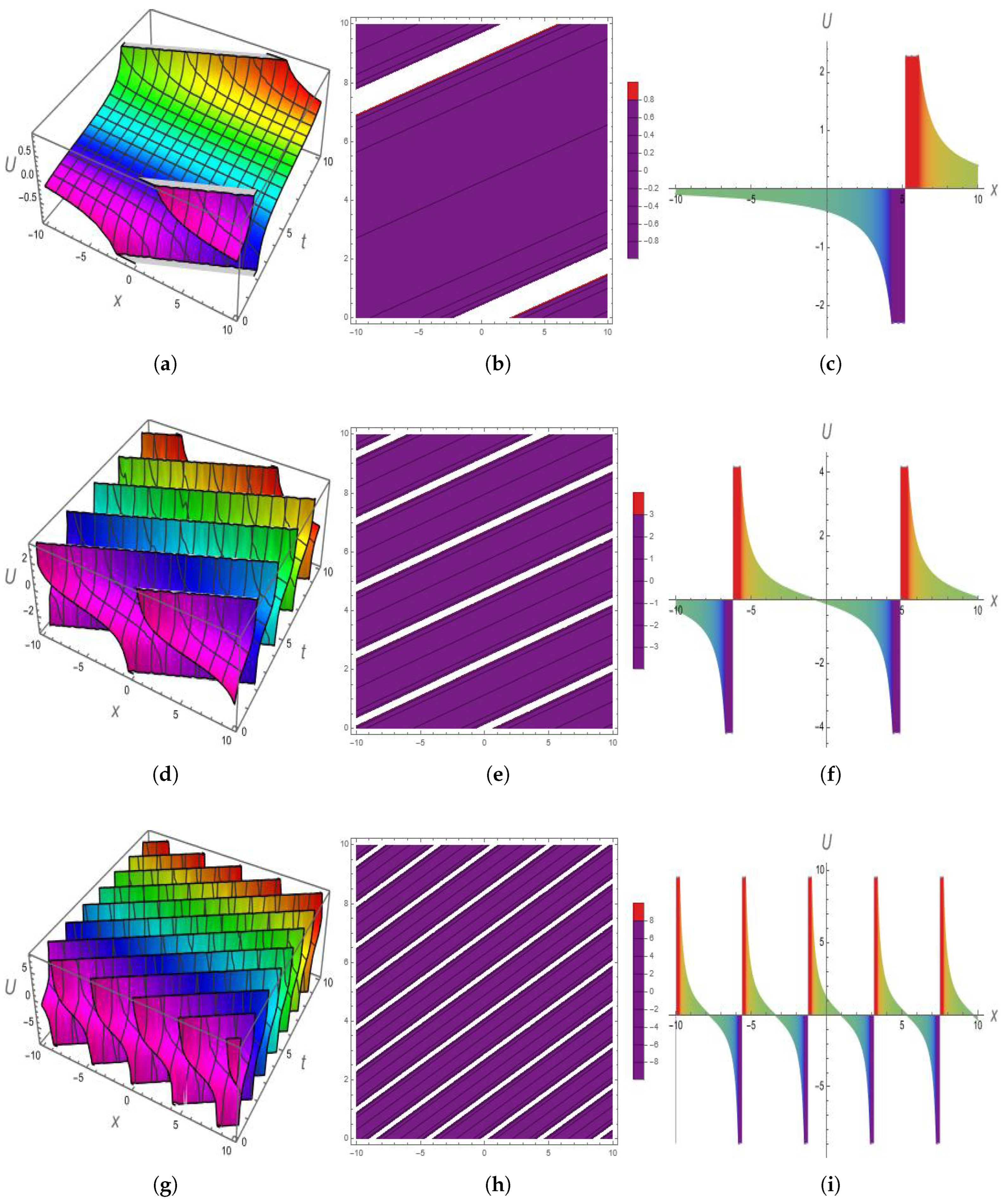
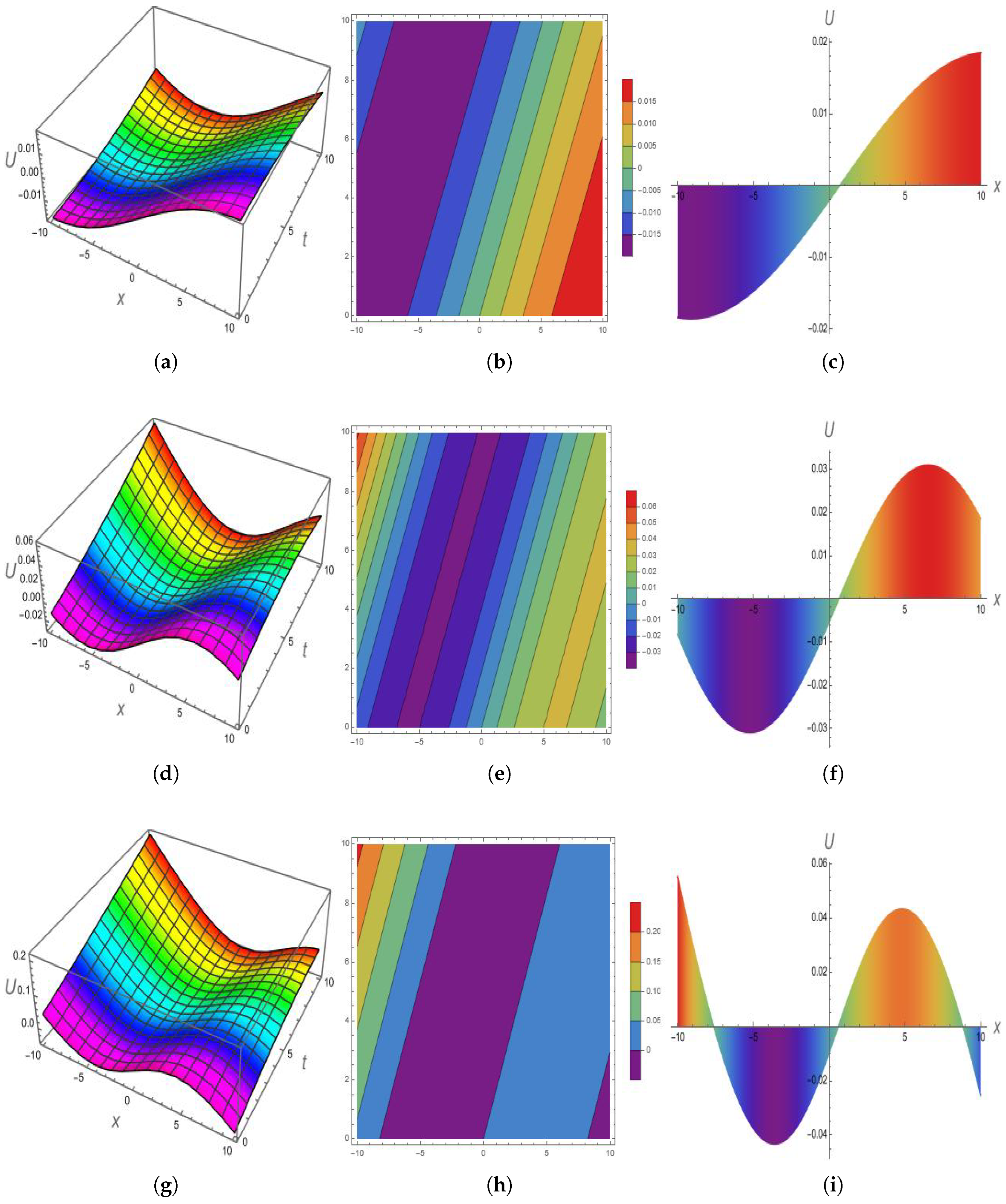
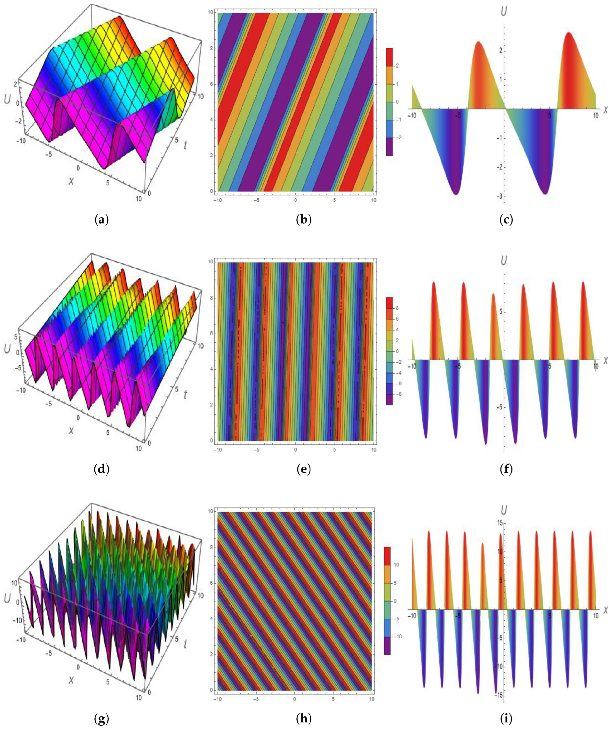
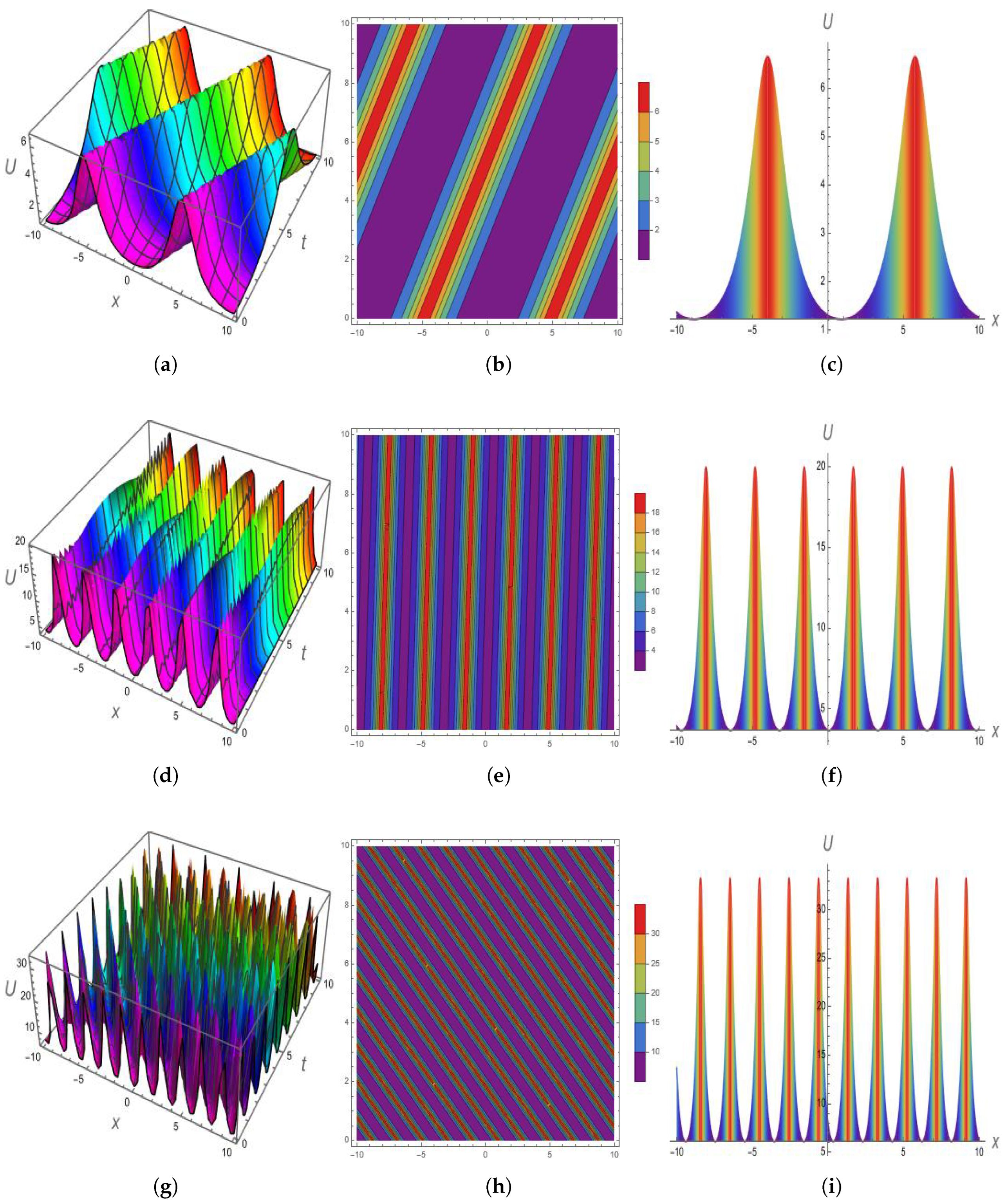
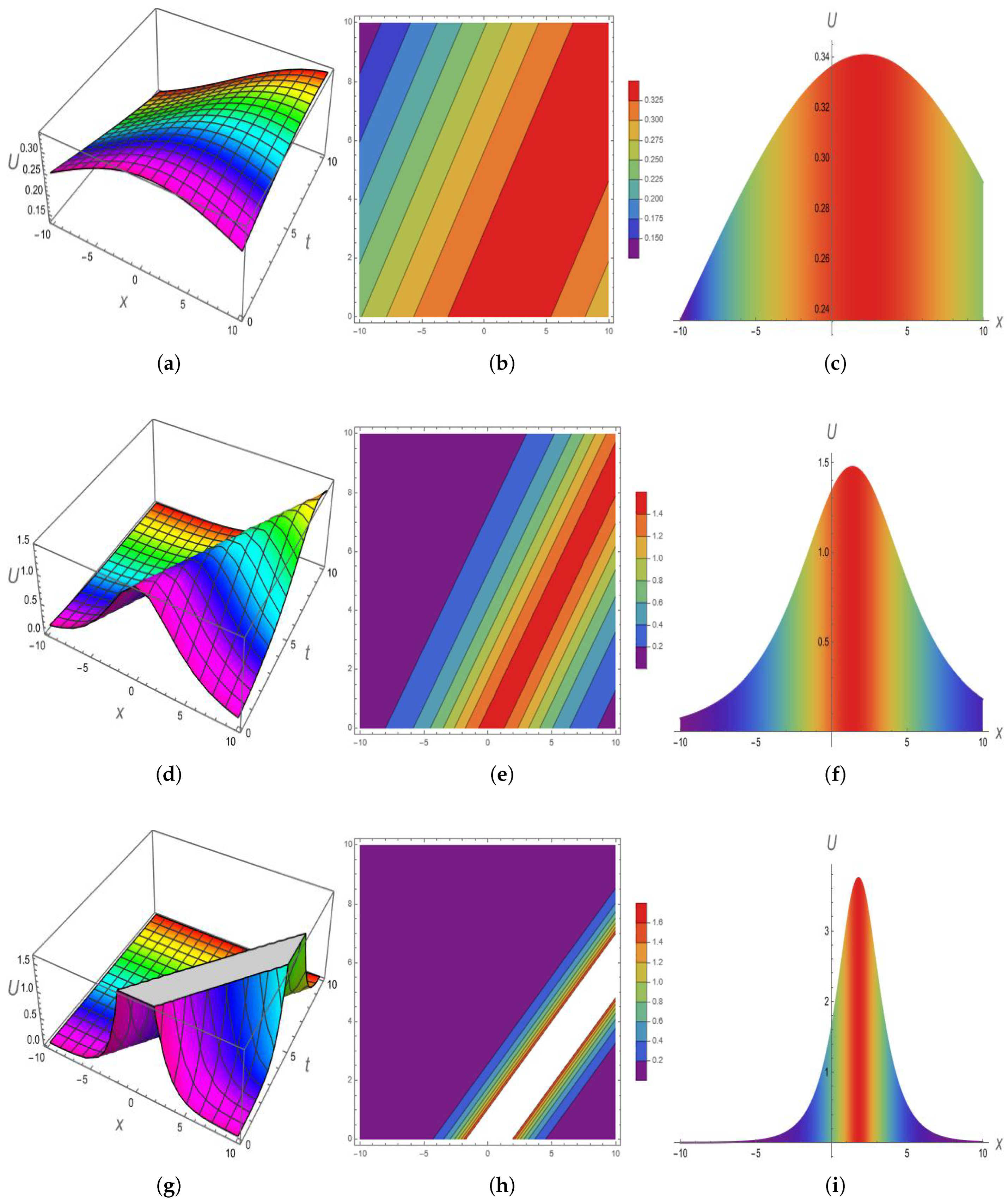
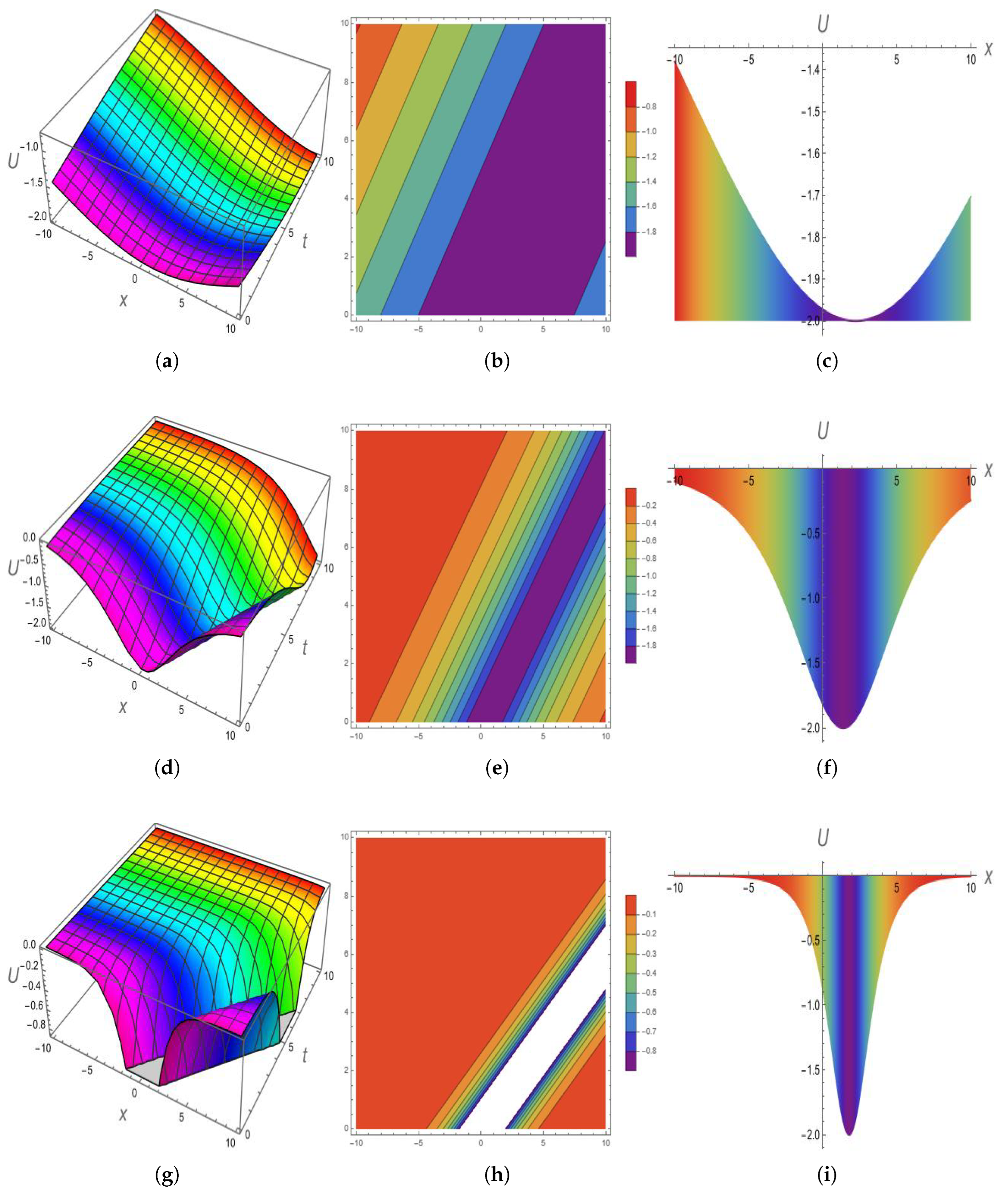
4. Graphical Discussion

This section is devoted to display and illustrating the graphic discussion and physical aspects of the obtained results.
Figure 1 displays the propagating behavior of solution  £ 3 , 2  with the parametric values  α = 0.1 , γ = 0.5 , β = 0.1 , δ 1 = 0.2 ,  and  δ 2 = 5 . This solution predicts the antikink periodic behavior of a traveling soliton with an amplitude-increasing fashion and periodicity as the wave number increases.
Figure 2 displays the propagating behavior of solution  £ 4 , 3  with the parametric values  α = 0.1 , γ = 0.4 , β = 0.6 , δ 1 = 0.5 ,  and  δ 2 = 0.2 .  This solution predicts the kink periodic behavior of a traveling soliton with an amplitude-increasing fashion as the wave number increases.
Figure 3 displays the propagating behavior of the real part of solution  £ 3  with the parametric values  ψ = 0.5 , ρ = 5 , m = 5 , n = 2 ; = 4 , ϑ = 2 , δ 1 = 0.5 ,  and  δ 2 = 0.5 . This solution predicts the periodic with antipeaked crests and antitroughs behavior of a traveling soliton with an amplitude-increasing fashion and periodicity as wave number increases.
Figure 4 displays the propagating behavior of the imaginary part of solution  £ 3  with the parametric values  ψ = 0.5 , ρ = 5 , m = 5 , n = 2 , = 4 , ϑ = 2 , δ 1 = 0.5 ,  and  δ 2 = 0.5 .  This solution predicts the periodic with peaked crests and troughs behavior of a traveling soliton with an amplitude-increasing fashion and periodicity as the wave number increases.
Figure 5 displays the propagating behavior of the real part of solution  £ 18  with the parametric values  ψ = 0.02 , = 0.3 , ρ = 5 , m = 5 , n = 6 , δ 1 = 0.5 ,  and  δ 2 = 0.5 .  This solution predicts the bright compacton with an amplitude-increasing fashion and the compacton achieves singularity as the wave number increases.
Figure 6 displays the propagating behavior of the imaginary part of solution  £ 18  with the parametric values  ψ = 0.02 , = 0.3 , ρ = 5 , m = 5 , n = 6 , δ 1 = 0.5 ,  and  δ 2 = 0.5 .  This solution predicts the dark compacton with an amplitude-increasing fashion and the compacton achieves singularity as the wave number increases.

5. Results and Novelty

This section presents the comparison and novelty of this study.
In the recent literature [45], authors developed the trigonometric, singular, periodic, hyperbolic, and kink solitons while in this study, singular solutions, mixed complex solitary shock solutions, mixed singular solutions, mixed shock singular solutions, mixed trigonometric solutions, mixed periodic solutions, mixed hyperbolic, antikink periodic, kink periodic, periodic with antipeaked crests and antitroughs, periodic with peaked crests and troughs, bright compacton, and dark compacton were found which were more generalized solutions. To our best knowledge, these types of soliton had not been studied before this study.
The result in this study was
£ 28 a ( x , y , t ) = k ψ log 2 ( ρ ) m n sinh ( 2 ψ Ω ) 2 ( m 2 n 2 tanh ( 2 ψ Ω ) 2 m n ψ Ω + 4 ψ Ω m n sinh ( 2 ψ Ω ) 5 m n tanh ( 2 ψ Ω ) + 2 ( m n ) 3 / 2 sec h ( 2 ψ Ω ) + 2 ψ Ω 2 m n sinh ( 2 ψ Ω ) + m n + sinh 2 ( 2 ψ Ω ) + m n sinh 2 ( 2 ψ Ω ) tanh ( 2 ψ Ω ) 2 ( m n ) 3 / 2 sinh ( 2 ψ Ω ) tanh ( 2 ψ Ω ) + 4 m n sinh ( 2 ψ Ω ) tanh ( 2 ψ Ω ) 2 ψ Ω sinh 2 ( 2 ψ Ω ) sinh 2 ( 2 ψ Ω ) tanh ( 2 ψ Ω ) ) ,
while the result from the literature (see Equation (29) in [45]) was
g f ( ρ ) = μ γ + ( μ 2 ν γ ) γ tanh ( ( μ 2 ν γ ) 2 ) ( k ( x + y ) + c t ) .
In the above solutions, it is clear that this study presented the more generalized and novel solutions. One can compare more results adopting the same process.

6. Conclusions

The generalized Calogero–Bogoyavlenskii–Schiff equation was investigated and analyzed by analytical techniques to obtain and visualize some deep insights. A combination of the new extended direct algebraic method and modified auxiliary equation method was applied and thus:
  • Numerous types of solitons were obtained which covered almost all kinds of solitary waves, such as singular solutions, mixed complex solitary shock solutions, mixed singular solutions, mixed shock singular solutions, mixed trigonometric solutions, mixed periodic solutions, and mixed hyperbolic solutions.
  • The real and imaginary wave propagation of the complex solutions was graphically displayed. The antikink periodic, kink periodic, periodic with antipeaked crests and antitroughs, periodic with peaked crests and troughs, bright compacton, and dark compacton behavior were graphically visualized.
  • Two-dimensional, 3D, and contour visualization were presented and we observed the influence of the parameters on the traveling behavior of the obtained solutions.
  • The wave number of the traveling wave profile was responsible for the control of the amplitude and the traveling behavior of the solitary wave. The singularity of the soliton wave could be controlled by the wave number parameter.
It is hoped that this study will be useful to researchers and analysts for improving experimental work; it can be extended to include multiple solitons, lump interaction, and rogue wave breathers.

Author Contributions

Formal analysis and problem formulation, W.A.F.; investigation and methodology, M.A.B., B.A.A. and W.A.F.; supervision, funding, and resources, A.-C.T., A.A. and M.S.; validation, graphical discussion, and software, A.-C.T. and W.A.F.; review and editing, B.A.A., W.A.F., A.-C.T. and M.S. All authors have read and agreed to the published version of the manuscript.

Funding

This research received no external funding.

Informed Consent Statement

Not applicable.

Data Availability Statement

All the data are within the manuscript.

Acknowledgments

Basem Al Alwan extends his appreciation to the Deanship of Scientific Research at King Khalid University, KSA, for funding this work through a large research group program under grant number R.G.P2/214/43.

Conflicts of Interest

The authors declare no conflict of interest.

References

  1. Wang, X.; Akram, G.; Sadaf, M.; Mariyam, H.; Abbas, M. Soliton Solution of the Peyrard–Bishop–Dauxois Model of DNA Dynamics with M-Truncated and β-Fractional Derivatives Using Kudryashov’s R Function Method. Fractal Fract. 2022, 6, 616. [Google Scholar] [CrossRef]
  2. Asjad, M.I.; Aleem, M.; Ali, W.; Abubakar, M.; Jarad, F. Enhancement of heat and mass transfer of a physical model using Generalized Caputo fractional derivative of variable order and modified Laplace transform method. J. Math. Anal. Model. 2021, 2, 41–61. [Google Scholar] [CrossRef]
  3. Akram, G.; Sadaf, M.; Khan, M.A.U. Soliton solutions of the resonant nonlinear Schrödinger equation using modified auxiliary equation method with three different nonlinearities. Math. Comput. Simul. 2023, 206, 1–20. [Google Scholar] [CrossRef]
  4. Abbas, M.; Bibi, A.; Alzaidi, A.S.; Nazir, T.; Majeed, A.; Akram, G. Numerical Solutions of Third-Order Time-Fractional Differential Equations Using Cubic B-Spline Functions. Fractal Fract. 2022, 6, 528. [Google Scholar] [CrossRef]
  5. Sajid, N.; Perveen, Z.; Sadaf, M.; Akram, G.; Abbas, M.; Abdeljawad, T.; Alqudah, M.A. Implementation of the Exp-function approach for the solution of KdV equation with dual power law nonlinearity. Comput. Appl. Math. 2022, 41, 338. [Google Scholar] [CrossRef]
  6. Algehyne, E.A.; Abd El-Rahman, M.; Faridi, W.A.; Asjad, M.I.; Eldin, S.M. Lie point symmetry infinitesimals, optimal system, power series solution, and modulational gain spectrum to the mathematical Noyes–Field model of nonlinear homogeneous oscillatory Belousov–Zhabotinsky reaction. Results Phys. 2023, 44, 106123. [Google Scholar] [CrossRef]
  7. Iqbal, M.S.; Yasin, M.W.; Ahmed, N.; Akgül, A.; Rafiq, M.; Raza, A. Numerical simulations of nonlinear stochastic Newell-Whitehead-Segel equation and its measurable properties. J. Comput. Appl. Math. 2023, 418, 114618. [Google Scholar] [CrossRef]
  8. Modanli, M.; Göktepe, E.; Akgül, A.; Alsallami, S.A.; Khalil, E.M. Two approximation methods for fractional order Pseudo-Parabolic differential equations. Alex. Eng. J. 2022, 61, 10333–10339. [Google Scholar] [CrossRef]
  9. Qureshi, Z.A.; Bilal, S.; Khan, U.; Akgül, A.; Sultana, M.; Botmart, T.; Zahran, H.Y.; Yahia, I.S. Mathematical analysis about influence of Lorentz force and interfacial nano layers on nanofluids flow through orthogonal porous surfaces with injection of SWCNTs. Alex. Eng. J. 2022, 61, 12925–12941. [Google Scholar] [CrossRef]
  10. Faridi, W.A.; Asghar, U.; Asjad, M.I.; Zidan, A.M.; Eldin, S.M. Explicit propagating electrostatic potential waves formation and dynamical assessment of generalized Kadomtsev–Petviashvili modified equal width-Burgers model with sensitivity and modulation instability gain spectrum visualization. Results Phys. 2023, 44, 106167. [Google Scholar] [CrossRef]
  11. Faridi, W.A.; Asjad, M.I.; Jhangeer, A.; Yusuf, A.; Sulaiman, T.A. The weakly non-linear waves propagation for Kelvin–Helmholtz instability in the magnetohydrodynamics flow impelled by fractional theory. Opt. Quantum Electron. 2023, 55, 172. [Google Scholar] [CrossRef] [PubMed]
  12. Faridi, W.A.; Asjad, M.I.; Jarad, F. The fractional wave propagation, dynamical investigation, and sensitive visualization of the continuum isotropic bi-quadratic Heisenberg spin chain process. Results Phys. 2022, 43, 106039. [Google Scholar] [CrossRef]
  13. Abu Bakar, M.; Owyed, S.; Faridi, W.A.; El-Rahman, A.; Sallah, M. The First Integral of the Dissipative Nonlinear Schrödinger Equation with Nucci’s Direct Method and Explicit Wave Profile Formation. Fractal Fract. 2023, 7, 38. [Google Scholar] [CrossRef]
  14. Faridi, W.A.; Asjad, M.I.; Jarad, F. Non-linear soliton solutions of perturbed Chen-Lee-Liu model by Φ 6-model expansion approach. Opt. Quantum Electron. 2022, 54, 664. [Google Scholar] [CrossRef]
  15. Asjad, M.I.; Faridi, W.A.; Jhangeer, A.; Ahmad, H.; Abdel-Khalek, S.; Alshehri, N. Propagation of some new traveling wave patterns of the double dispersive equation. Open Phys. 2022, 20, 130–141. [Google Scholar] [CrossRef]
  16. Almusawa, H.; Jhangeer, A. A study of the soliton solutions with an intrinsic fractional discrete nonlinear electrical transmission line. Fractal Fract. 2022, 6, 334. [Google Scholar] [CrossRef]
  17. Fahim, M.R.A.; Kundu, P.R.; Islam, M.E.; Akbar, M.A.; Osman, M.S. Wave profile analysis of a couple of (3+1)-dimensional nonlinear evolution equations by sine-Gordon expansion approach. J. Ocean. Eng. Sci. 2022, 7, 272–279. [Google Scholar] [CrossRef]
  18. Akinyemi, L.; Şenol, M.; Osman, M.S. Analytical and approximate solutions of nonlinear Schrödinger equation with higher dimension in the anomalous dispersion regime. J. Ocean. Eng. Sci. 2022, 7, 143–154. [Google Scholar] [CrossRef]
  19. Liu, J.G.; Osman, M.S. Nonlinear dynamics for different nonautonomous wave structures solutions of a 3D variable-coefficient generalized shallow water wave equation. Chin. J. Phys. 2022, 77, 1618–1624. [Google Scholar] [CrossRef]
  20. Baber, M.Z.; Seadway, A.R.; Iqbal, M.S.; Ahmed, N.; Yasin, M.W.; Ahmed, M.O. Comparative analysis of numerical and newly constructed soliton solutions of stochastic Fisher-type equations in a sufficiently long habitat. Int. J. Mod. Phys. B 2022, 2350155. [Google Scholar] [CrossRef]
  21. Rehman, H.U.; Seadawy, A.R.; Younis, M.; Rizvi, S.T.R.; Anwar, I.; Baber, M.Z.; Althobaiti, A. Weakly nonlinear electron-acoustic waves in the fluid ions propagated via a (3+1)-dimensional generalized Korteweg–de-Vries–Zakharov–Kuznetsov equation in plasma physics. Results Phys. 2022, 33, 105069. [Google Scholar] [CrossRef]
  22. Kumar, S.; Dhiman, S.K. Lie symmetry analysis, optimal system, exact solutions and dynamics of solitons of a (3+1)-dimensional generalised BKP–Boussinesq equation. Pramana 2022, 96, 31. [Google Scholar] [CrossRef]
  23. Kumar, S.; Dhiman, S.K.; Baleanu, D.; Osman, M.S.; Wazwaz, A.M. Lie symmetries, closed-form solutions, and various dynamical profiles of solitons for the variable coefficient (2+1)-dimensional KP equations. Symmetry 2022, 14, 597. [Google Scholar] [CrossRef]
  24. Wazwaz, A.M. Bright and dark optical solitons of the (2+1)-dimensional perturbed nonlinear Schrödinger equation in nonlinear optical fibers. Optik 2022, 251, 168334. [Google Scholar] [CrossRef]
  25. Wazwaz, A.M.; Albalawi, W.; El-Tantawy, S.A. Optical envelope soliton solutions for coupled nonlinear Schrödinger equations applicable to high birefringence fibers. Optik 2022, 255, 168673. [Google Scholar] [CrossRef]
  26. Wazwaz, A.M.; El-Tantawy, S.A. Bright and dark optical solitons for (3+1)-dimensional hyperbolic nonlinear Schrödinger equation using a variety of distinct schemes. Optik 2022, 270, 170043. [Google Scholar] [CrossRef]
  27. Tariq, K.U.; Wazwaz, A.M.; Ahmed, A. On some optical soliton structures to the Lakshmanan-Porsezian-Daniel model with a set of nonlinearities. Opt. Quantum Electron. 2022, 54, 432. [Google Scholar] [CrossRef]
  28. Seadawy, A.R.; Rizvi, S.T.; Akram, U.; Naqvi, S.K. Optical and analytical soliton solutions to higher order non-Kerr nonlinear Schrödinger dynamical model. J. Geom. Phys. 2022, 179, 104616. [Google Scholar] [CrossRef]
  29. Rizvi, S.T.; Seadawy, A.R.; Akram, U. New dispersive optical soliton for an nonlinear Schrödinger equation with Kudryashov law of refractive index along with P-test. Opt. Quantum Electron. 2022, 54, 310. [Google Scholar] [CrossRef]
  30. Younis, M.; Bilal, M.; Rehman, S.U.; Seadawy, A.R.; Rizvi, S.T.R. Perturbed optical solitons with conformable time-space fractional Gerdjikov–Ivanov equation. Math. Sci. 2022, 16, 431–443. [Google Scholar] [CrossRef]
  31. Tariq, K.U.; Seadawy, A.R.; Rizvi, S.T.; Javed, R. Some optical soliton solutions to the generalized (1+1)-dimensional perturbed nonlinear Schrödinger equation using two analytical approaches. Int. J. Mod. Phys. B 2022, 36, 2250177. [Google Scholar] [CrossRef]
  32. Bu, L.; Baronio, F.; Chen, S.; Trillo, S. Quadratic Peregrine solitons resonantly radiating without higher-order dispersion. Opt. Lett. 2022, 47, 2370–2373. [Google Scholar] [CrossRef]
  33. Shen, S.; Yang, Z.J.; Pang, Z.G.; Ge, Y.R. The complex-valued astigmatic cosine-Gaussian soliton solution of the nonlocal nonlinear Schrödinger equation and its transmission characteristics. Appl. Math. Lett. 2022, 125, 107755. [Google Scholar] [CrossRef]
  34. Song, L.M.; Yang, Z.J.; Li, X.L.; Zhang, S.M. Coherent superposition propagation of Laguerre–Gaussian and Hermite–Gaussian solitons. Appl. Math. Lett. 2020, 102, 106114. [Google Scholar] [CrossRef]
  35. Guo, J.L.; Yang, Z.J.; Song, L.M.; Pang, Z.G. Propagation dynamics of tripole breathers in nonlocal nonlinear media. Nonlinear Dyn. 2020, 101, 1147–1157. [Google Scholar] [CrossRef]
  36. Yang, Z.J.; Zhang, S.M.; Li, X.L.; Pang, Z.G.; Bu, H.X. High-order revivable complex-valued hyperbolic-sine-Gaussian solitons and breathers in nonlinear media with a spatial nonlocality. Nonlinear Dyn. 2018, 94, 2563–2573. [Google Scholar] [CrossRef]
  37. Shen, S.; Yang, Z.; Li, X.; Zhang, S. Periodic propagation of complex-valued hyperbolic-cosine-Gaussian solitons and breathers with complicated light field structure in strongly nonlocal nonlinear media. Commun. Nonlinear Sci. Numer. Simul. 2021, 103, 106005. [Google Scholar] [CrossRef]
  38. Gonzalez-Gaxiola, O.; Biswas, A.; Ekici, M.; Khan, S. Highly dispersive optical solitons with quadratic–cubic law of refractive index by the variational iteration method. J. Opt. 2021, 51, 29–36. [Google Scholar] [CrossRef]
  39. Aniqa, A.; Ahmad, J. Soliton solution of fractional Sharma-Tasso-Olever equation via an efficient ( G G )-expansion method. Ain Shams Eng. J. 2022, 13, 101528. [Google Scholar] [CrossRef]
  40. Zagorac, J.L.; Sands, I.; Padmanabhan, N.; Easther, R. Schrödinger-Poisson solitons: Perturbation theory. Phys. Rev. D 2022, 105, 103506. [Google Scholar] [CrossRef]
  41. Bettelheim, E.; Smith, N.R.; Meerson, B. Inverse scattering method solves the problem of full statistics of nonstationary heat transfer in the Kipnis-Marchioro-Presutti model. Phys. Rev. Lett. 2022, 128, 130602. [Google Scholar] [CrossRef] [PubMed]
  42. Zhang, Y.; Dang, S.; Li, W.; Chai, Y. Performance of the radial point interpolation method (RPIM) with implicit time integration scheme for transient wave propagation dynamics. Comput. Math. Appl. 2022, 114, 95–111. [Google Scholar] [CrossRef]
  43. Younas, U.; Sulaiman, T.A.; Ren, J. Diversity of optical soliton structures in the spinor Bose–Einstein condensate modeled by three-component Gross–Pitaevskii system. Int. J. Mod. Phys. B 2023, 37, 2350004. [Google Scholar] [CrossRef]
  44. Yao, S.W.; Akram, G.; Sadaf, M.; Zainab, I.; Rezazadeh, H.; Mustafa Inc. Bright, dark, periodic and kink solitary wave solutions of evolutionary Zoomeron equation. Results Phys. 2022, 43, 106117. [Google Scholar] [CrossRef]
  45. Jarad, F.; Jhangeer, A.; Awrejcewicz, J.; Riaz, M.B.; Junaid-U-Rehman, M. Investigation of wave solutions and conservation laws of generalized Calogero–Bogoyavlenskii–Schiff equation by group theoretic method. Results Phys. 2022, 37, 105479. [Google Scholar] [CrossRef]
Figure 1. Three-dimensional, contour, and 2-D profiles of solution  £ 3 , 2  for different values of parameter k. (a) Three-dimensional propagation at  k = 0.3 ; (b) Contour propagation at  k = 0.3 ; (c) Two-dimensional propagation at  k = 0.3 ; (d) Three-dimensional propagation at  k = 1.3 ; (e) Contour propagation at  k = 1.3 ; (f) Two-dimensional propagation at  k = 1.3 ; (g) Three-dimensional propagation at  k = 3.3 ; (h) Contour propagation at  k = 3.3 ; (i) Two-dimensional propagation at  k = 3.3 .
Fractalfract 07 00191 g001
Figure 2. Three-dimensional, contour, and 2-D profiles of solution  £ 4 , 3  for different values of parameter k. (a) Three-dimensional propagation at  k = 0.3 ; (b) Contour propagation at  k = 0.3 ; (c) Two-dimensional propagation at  k = 0.3 ; (d) Three-dimensional propagation at  k = 0.5 ; (e) Contour propagation at  k = 0.5 ; (f) Two-dimensional propagation at  k = 0.5 ; (g) Three-dimensional propagation at  k = 0.7 ; (h) Contour propagation at  k = 0.7 ; (i) Two-dimensional propagation at  k = 0.7 .
Fractalfract 07 00191 g002
Figure 3. Three-dimensional, contour and 2-D profiles for the real part of solution  £ 3  for different values of parameter k. (a) Three-dimensional propagation at  k = 0.1 ; (b) Contour propagation at  k = 0.1 ; (c) Two-dimensional propagation at  k = 0.1 ; (d) Three-dimensional propagation at  k = 0.3 ; (e) Contour propagation  k = 0.3 ; (f) Two-dimensional propagation  k = 0.3 ; (g) Three-dimensional propagation  k = 0.5 ; (h) Contour propagation  k = 0.5 ; (i) Two-dimensional propagation  k = 0.5 .
Fractalfract 07 00191 g003
Figure 4. Three-dimensional, contour, and 2-D profiles for the imaginary part of solution  £ 3  for different values of parameter k. (a) Three-dimensional propagation at  k = 0.1 ; (b) Contour propagation at  k = 0.1 ; (c) Two-dimensional propagation at  k = 0.1 ; (d) Three-dimensional propagation at  k = 0.3 ; (e) Contour propagation at  k = 0.3 ; (f) Two-dimensional propagation at  k = 0.3 ; (g) Three-dimensional propagation at  k = 0.5 ; (h) Contour propagation at  k = 0.5 ; (i) Two-dimensional propagation at  k = 0.5 .
Fractalfract 07 00191 g004
Figure 5. Three-dimensional, contour, and 2-D profiles for the real part of solution  £ 18  for different values of parameter k. (a) Three-dimensional propagation at  k = 0.3 ; (b) Contour propagation at  k = 0.3 ; (c) Two-dimensional propagation at  k = 0.3 ; (d) Three-dimensional propagation at  k = 1.3 ; (e) Contour propagation at  k = 1.3 ; (f) Two-dimensional propagation at  k = 1.3 ; (g) Three-dimensional propagation at  k = 3.3 ; (h) Contour propagation at  k = 3.3 ; (i) Two-dimensional propagation at  k = 3.3 .
Fractalfract 07 00191 g005
Figure 6. Three-dimensional, contour, and 2-D profiles for the imaginary part of solution  £ 18  for different values of parameter k. (a) Three-dimensional propagation at  k = 0.3 ; (b) Contour propagation at  k = 0.3 ; (c) Two-dimensional propagation at  k = 0.3 ; (d) Three-dimensional propagation at  k = 1.3 ; (e) Contour propagation at  k = 1.3 ; (f) Two-dimensional propagation at  k = 1.3 ; (g) Three-dimensional propagation at  k = 3.3 ; (h) Contour propagation at  k = 3.3 ; (i) Two-dimensional propagation at  k = 3.3 .
Fractalfract 07 00191 g006
Disclaimer/Publisher’s Note: The statements, opinions and data contained in all publications are solely those of the individual author(s) and contributor(s) and not of MDPI and/or the editor(s). MDPI and/or the editor(s) disclaim responsibility for any injury to people or property resulting from any ideas, methods, instructions or products referred to in the content.

