Article

On Fractional Order Model of Tumor Growth with Cancer Stem Cell

1
Faculty of Science, Shahid Rajaee Teacher Training University, Lavizan, Tehran 16785-163, Iran
2
School of Mathematics, Iran University of Science and Technology, Narmak, Tehran 16846-13114, Iran
3
Department of Mathematical Sciences, University of South Africa, Florida 0003, South Africa
*
Author to whom correspondence should be addressed.
Fractal Fract. 2023, 7(1), 27; https://doi.org/10.3390/fractalfract7010027
Submission received: 27 November 2022 / Revised: 21 December 2022 / Accepted: 22 December 2022 / Published: 27 December 2022

Abstract

:
This paper generalizes the integer-order model of the tumour growth into the fractional-order domain, where the long memory dependence of the fractional derivative can be a better fit for the cellular response. This model describes the dynamics of cancer stem cells and non-stem (ordinary) cancer cells using a coupled system of nonlinear integro-differential equations. Our analysis focuses on the existence and boundedness of the solution in correlation with the properties of Mittag-Leffler functions and the fixed point theory elucidating the proof. Some numerical examples with different fractional orders are shown using the finite difference scheme, which is easily implemented and reliably accurate. Finally, numerical simulations are employed to investigate the influence of system parameters on cancer progression and to confirm the evidence of tumour growth paradox in the presence of cancer stem cells.

1. Introduction

Cancer is one of the most complex diseases of the 21st century, characterized by the uncontrolled growth of abnormal cells in any organ of the body. Using mathematical models, we are able to simulate cancer mechanisms, propose and validate hypotheses, and develop therapeutic protocols; in other words, we can use mathematical models to forecast, realize, and improve cancer treatment. Generally, cancer treatment aims to eliminate as many non-stem cancer cells (NSCCs) as possible while minimizing damage to healthy cells around them. In the absence of correct elimination of enough cancer stem cells (CSCs), cancer therapies may fail to eliminate the tumour, and this strategy may fail. The “tumour growth paradox” occurs when cancer cells are subjected to an immune response or cytotoxic treatment; however, the tumour grows at a faster rate when the cancer cells die. In contrast, these processes cannot eliminate CSCs, and therapy may lead to increased tumour size instead [1,2].
Many papers have been proposed to describe the tumour evolution in the existence of cancer stem cells (CSCs) [1,2,3,4,5,6]. Hillen et al. [2] presented the birth-jump model as the following integro-differential system of PDEs in 2013 to explain the CSCs and NSCCs dynamics. The model includes that stem and non-stem cancer cells duplicate until some homeostatic state is achieved. Stem cells are sensitive to the total tumour size, whereas non-stem cancer cells only increase by nutrient limitation.
Considering the integro-differential system of PDEs in the following manner:
u ( x , t ) t = D u Δ u + γ δ Ω K u x , y , p ( x , t ) u ( y , t ) d y , v ( x , t ) t = D v Δ v α v ( x , t ) + γ ( 1 δ ) Ω K u x , y , p ( x , t ) u ( y , t ) d y + ρ Ω K v x , y , p ( x , t ) v ( y , t ) d y .
The initial conditions (ICs) are prescribed as:
u ( x , 0 ) = u 0 ( x ) 0 , v ( x , 0 ) = v 0 ( x ) 0 , u 0 ( x ) + v 0 ( x ) 1 , x Ω .
Borsi and Fasano explored the system (1) and proved the unique and bounded solution’s existence as well as presented helpful results in the local and global existence of the solutions [3,4]. Additionally, Maddalena [5,7] investigated the stability of steady states about the above system and proved that a limited invariant set exists in the positive zone, giving a global solution.
In recent years, the mathematical modelling of infectious disease as a fractional-order system of equations has increased concentration [8,9,10,11]. As fractional-order models are more factual than integer-order models, mathematicians are motivated to apply fractional-order ones. This paper presents a model describing memory effects (time) and nonlocal phenomena (space) accurately. One of the most important benefit of fractional-order models is the reduction of errors associated with the omission of parameters in natural phenomena. We apply time-fractional derivatives to simulate tumour evolution in the presence of cancer stem cells. This model is the generalization of integer-order model (1) which was analyzed by Hillen [2]. The objective of this study is to investigate the sensitivity of the cancer growth paradox to the different mortality rates of NSCCs and demonstrate that the paradox occurs for different parameter values in the proposed model.
This paper is organized as follows. Section 2 describes some basic fractional calculus definitions. Section 3 proposes the fractional-order model. Section 4 shows some properties of global and local uniqueness and existence, positivity, and boundedness of solutions. Section 5 reports the numerical results in order to confirm the cancer growth paradox. Finally, Section 6 summarizes the concluding remarks.

2. Basic Definitions

Fractional calculus is an efficient tool for simulating biological systems. The fractional-order derivation has been defined in several ways such as the Riemann–Liouville definition, the Caputo definition, the Riesz derivative, the local fractional derivative, He’s fractional derivative, conformable fractional derivative and so on [12,13,14,15,16]. A Riemann–Liouville definition and a Caputo definition are the most commonly used [17,18,19,20,21,22,23]. Some basic fractional calculus definitions and notations have been given in this section.
Definition 1.
The Riemann–Liouville fractional (RL) integral operator I β f of order β for a continuous function f L 1 [ 0 , t ] , s [ 0 , t ] (as usual L 1 is the set of Lebesgue integrable functions) is presented as
I β f ( t ) = 1 Γ ( β ) 0 t ( t s ) β 1 f ( s ) d s ,
in which Γ ( · ) is the well-known Euler’s Gamma function.
Definition 2.
The inverse of I β f ( t ) operator, is the RL fractional derivative:
D β f ( t ) = 1 Γ ( n β ) d d t n 0 t ( t s ) n β 1 f ( s ) d s .
An alternative illustration of the fractional derivative received after changing differentiation and integration in (2).
Definition 3.
The Caputo’s time fractional derivative operator D β of order β for a function f is defined as:
D β f ( t ) = 1 Γ ( n β ) 0 t ( t s ) n β 1 f ( n ) ( s ) d s ,
where β ( n 1 , n ) , n N . Particularly, when β ( 0 , 1 ) it holds:
D β f ( t ) = 1 Γ ( n β ) 0 t f ( s ) ( t s ) β d s .
Both the Caputo and the Riemann–Liouville derivatives are mainly used in fractional differential equations (FDEs). In the former, the initial value of the fractional-order differential equation with Caputo derivative is similar to the integer-order differential equation and is not determined locally at time t. Considering the initial value conditions imposed on the fractional differential equation and the nature of the problem, we choose one of the above definitions. Caputo reformulated the definition of the Riemann-Liouville fractional derivative by switching the order of the ordinary derivative with the fractional integral operator. Thus, the Caputo derivative’s Laplace transform depends on integer order initial conditions, whereas Riemann–Liouville fractional derivatives depend on fractional order initial conditions. Using the Caputo fractional derivative allows the formulation of the problem to include traditional initial and boundary conditions [24,25]. We consider the Caputo derivative with fractional-order instead of integer-order derivative throughout this paper to reformulate and analyze the system (1).
Definition 4.
The well-known Mittag-Leffler function of order β is defined by
E β ( z ) : = n = 0 z n Γ ( n β + 1 ) , β > 0 , z C ,
where the series convergent in the whole complex plane. This function has been introduced by Mittag-Leffler and is a direct generalization of the exponential function. Immediately notice that for β = 1 , we have the exponential series
E 1 ( z ) = n = 0 z n Γ ( n + 1 ) = j = 0 z n n ! = exp ( z ) , z C .
which is the exponential function [26].
Among the various results on Mittag-Leffler functions, the critical one dealing with asymptotic expansions of these functions is directly practical in the solution of the FDEs and the analysis of the behaviour of the solution for large and small values of the argument. Simply to say, physical laws could control derivations of physical phenomena from exponential behaviour through Mittag-Leffler functions.

3. The Fractional Model

The integer-order model of tumour growth based on the CSCs was proposed by Ref. [2] as an integral-partial differential system (1). This paper discusses the generalized fractional-order model of tumour growth. Fractional-order elements have the following two main advantages:
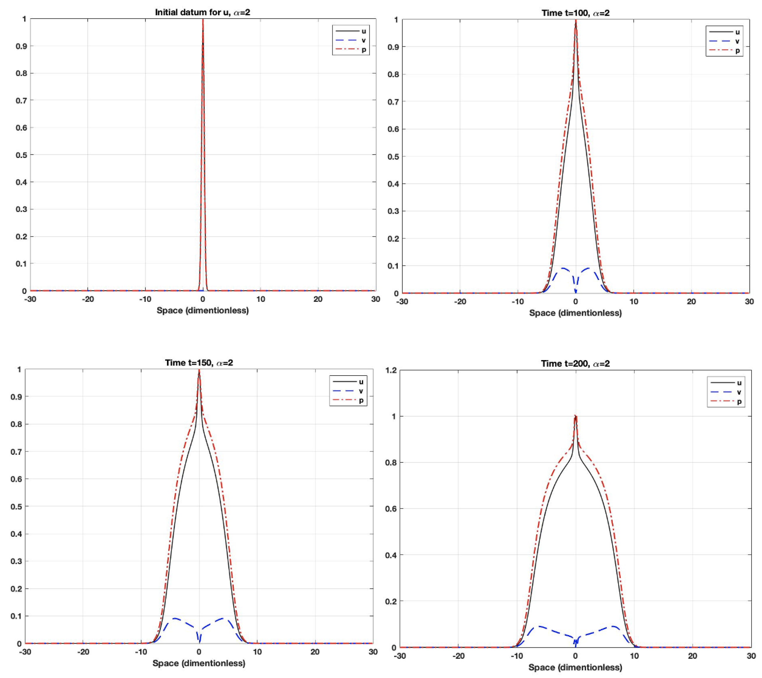
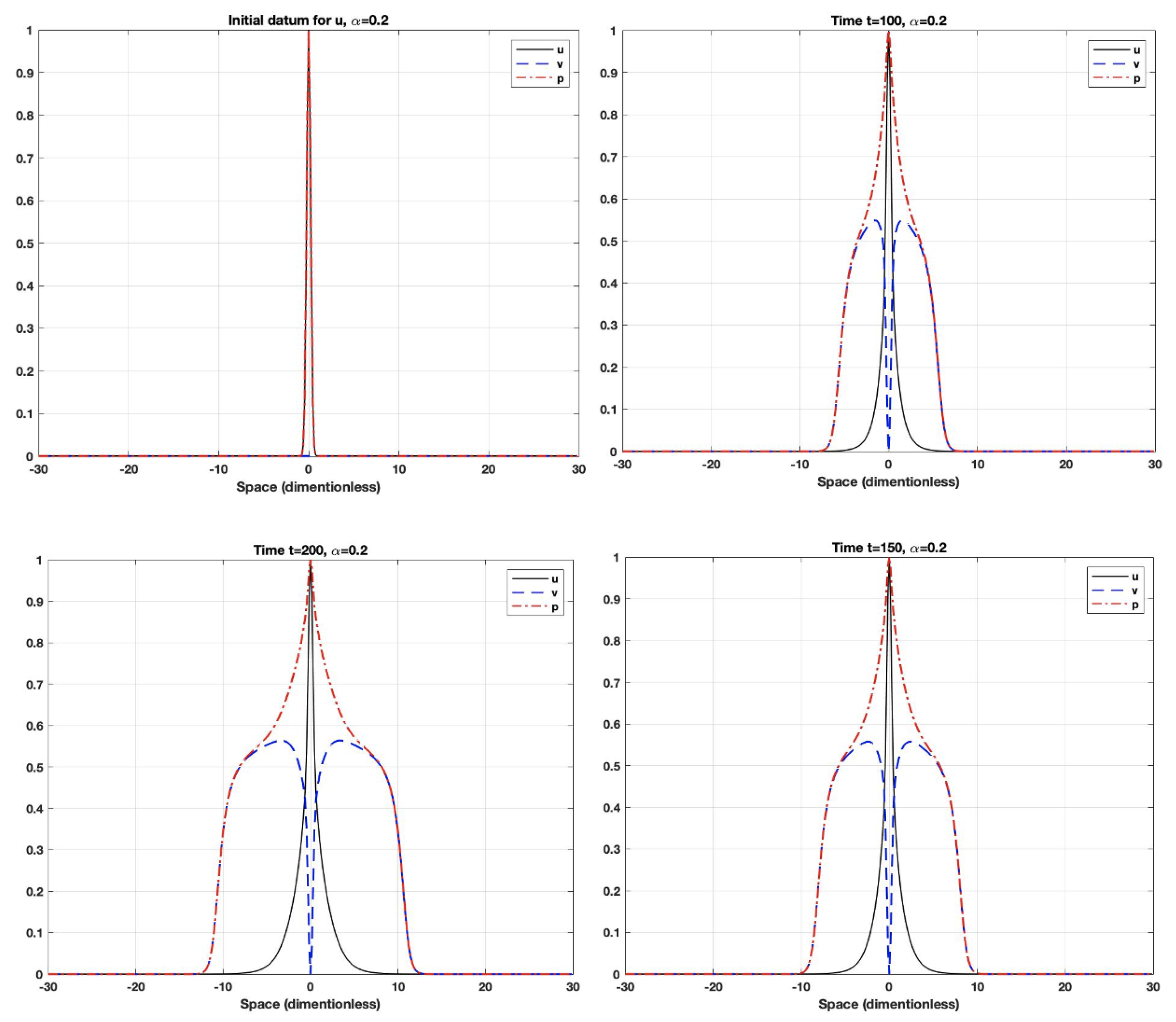
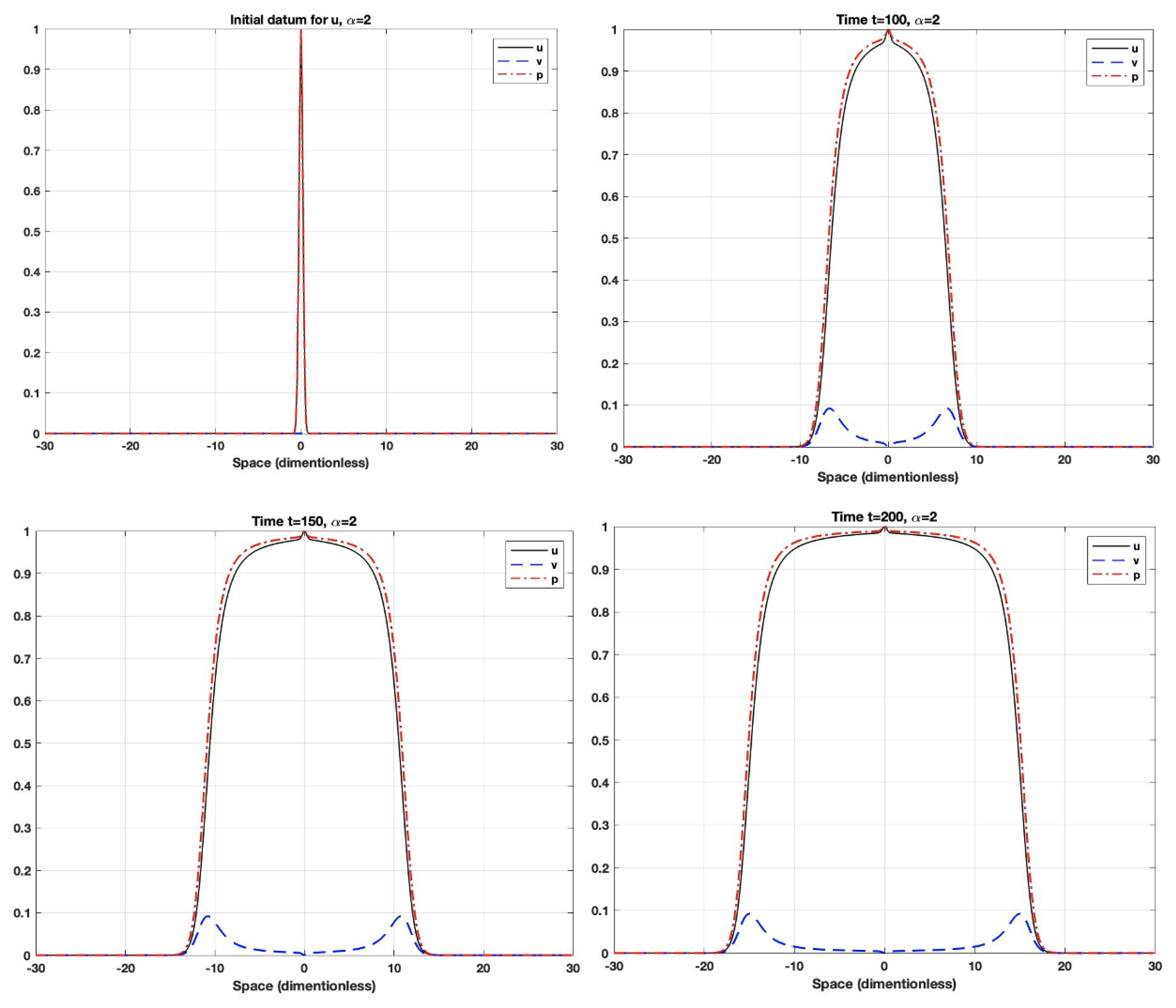
  • The fractional derivative is a long-term operator, which means that the system response at any time will be affected by all previous responses. Additionally, the fractional-order parameter could control the dependence on the previous response (i.e., memory). When the order is small, the system uses the previous cases more often than it does when the order gets closer to one. As the order gets closer to one, the system will have a shorter memory dependence.
  • Using fractional-order parameters enhances the system performance by increasing the degree of freedom. This allows the system to extend to a larger area.
Thus, we replace the first-order derivatives with the Caputo fractional derivative and assume that there is no diffusion term, like [3]. Several interpretations of fractional calculus exist [12,27] However, they are usually abstract and lack physical intuition. The interpretation we have provided is therefore the most useful interpretation available for fractional calculus. A key component of these interpretations is the concept of memory. A memoryless system is one whose output depends only on its input at each time t. However, when the output depends on the previous value of the input, such systems are said to be memory systems. Since fractional derivatives rely on long memory, they can provide a better fit for cellular response. Furthermore, we consider a positive coefficient 1 λ 1 β including λ as an auxiliary parameter to prevent dimensional mismatching [28]. Therefore, the system can be reduced to the following form:
1 λ 1 β β u ( x , t ) t β = γ δ Ω K u x , y , p ( x , t ) u ( y , t ) d y ,
1 λ 1 β β v ( x , t ) t β = α v ( x , t ) + γ ( 1 δ ) Ω K u x , y , p ( x , t ) u ( y , t ) d y + ρ Ω K v x , y , p ( x , t ) v ( y , t ) d y .
The ICs are given as:
u ( x , 0 ) = u 0 ( x ) 0 ,
v ( x , 0 ) = v 0 ( x ) 0 ,
u 0 ( x ) + v 0 ( x ) 1 , x Ω .
  • The term K ( x , y , p ( x , t ) ) shows the probability density of the tumour cell (CSCs or NSCCs) that a mother cell located at y generates a daughter cell at the position x. As cell distribution only takes place inside the domain Ω , the kernel of integral equals zero for all x Ω . Note that K ( x , y , p ( x , t ) ) 1 , since it is impossible to distribute more than one cell per cell cycle. Let Ω K ( x , y , p ( x , t ) ) d y 1 , because this integration represents the total distribution of the cells in the whole domain. Furthermore, K ( x , y , p ( x , t ) ) stands for a monotonically decreasing function (with the variables x and y). Due to the fact that the probability increases when the cells are close to each other and decreases when the cells are far apart. Thus, the distribution kernel depends on the total cell population at x, i.e., p ( x , t ) , causes the volume effect, which describes the more value of p is at node ( x , t ) , the lower probability of the cell generation is at that one node [4]. Therefore, the integral kernel can be considered separable:
    K ( x , y , p ( x , t ) ) = F ( p ( x , t ) ) K ( x , y ) ,
    in which 0 K C ( Ω × Ω ) . It should be noticed that F ( p ) C 1 is a non-increasing, non-negative and strictly decreasing when p = 1 . F ( p ) denotes continuous Lipschitz function in [ 0 , 1 ] including F ( 0 ) = 1 , F ( 1 ) = 0 . We suppose that function K ( x , y ) shows the distance between the two nodal points x and y, that is, K ( x , y ) = K ( | x y | ) , x , y Ω R n . Furthermore, we can consider the arguments of K ( x , y ) with “small” variances. An obvious example is the Gaussian distribution kernel
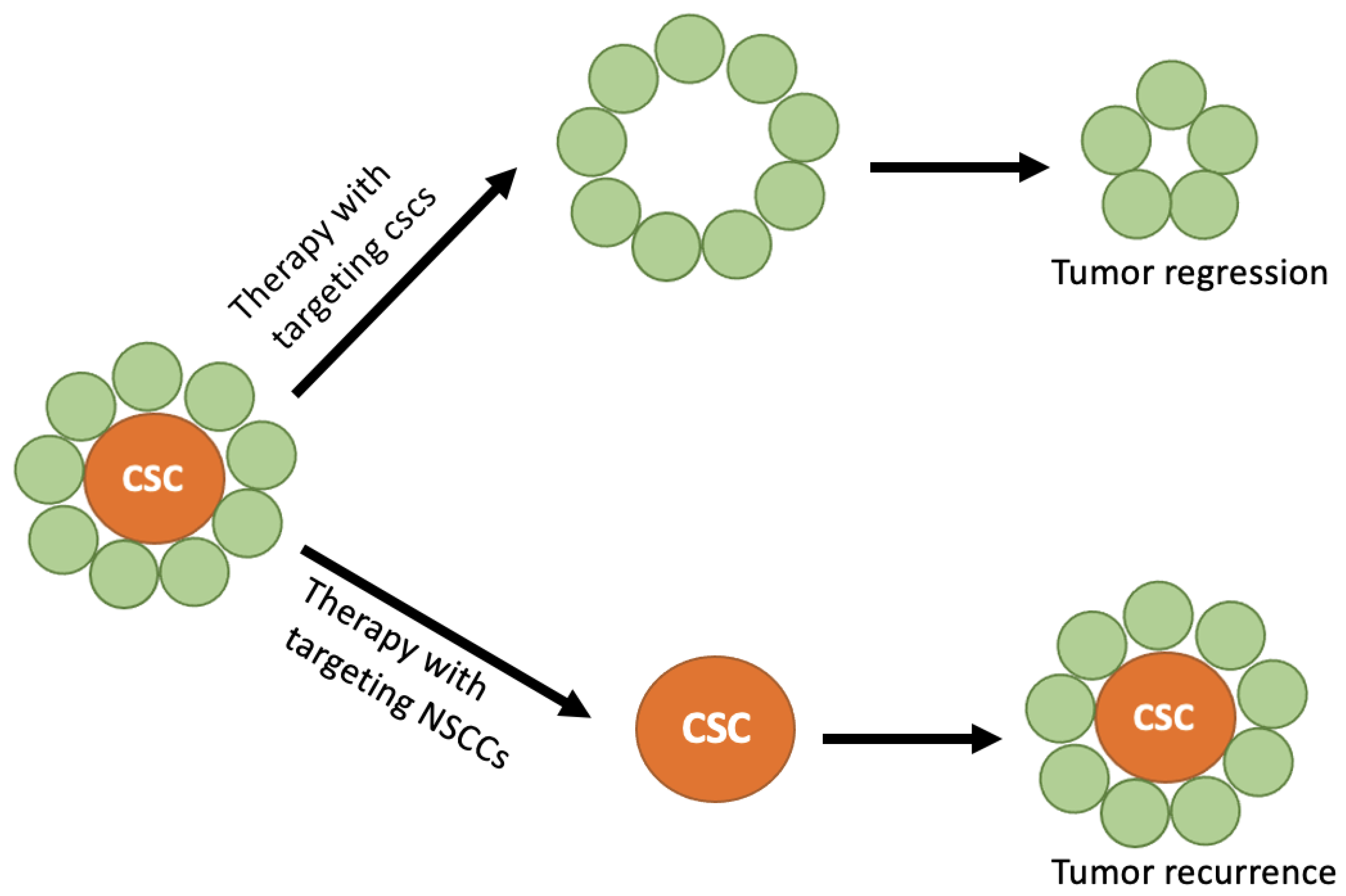
    K ( x , y ) = 1 σ π exp ( x y ) 2 / σ v 2
  • The terms v ( x , t ) and u ( x , t ) denote the density of CSCs and CCs, respectively and also p ( x , t ) = v ( x , t ) + u ( x , t ) shows the density of tumour cells.
Table 1 lists the meanings of the parameters in the above system. Figure 1 shows distinction between CSC-targeted therapy and NSCC-targeted therapy.

4. Existence and Uniqueness Analysis

The current section is devoted to showing the dependence of the ICs on the existence of the solutions. As a next step, we prove the uniqueness, existence, and boundedness of the local and global solutions for the proposed mathematical tumour growth model.
Lemma 1.
Under assumption (6) any solution of (4) and (5) has a priori bound.
Proof. 
We define the following norms to obtain prior estimates on bounds of v and u.
u ( x , t ) t = max Ω ^ × [ 0 , t ] | u ( x , s ) | , v ( x , t ) t = max Ω ^ × [ 0 , t ] | v ( x , s ) | .
Applying the RL fractional integral operator with order β to both sides of (4) and taking maximum value of F, we find
u ( x , t ) t max x Ω ^ | u 0 | + γ δ Γ ( β ) 0 t ( t s ) β 1 u s d s .
The generalized Gronwall’s inequality [29] results in
u ( x , t ) t max x Ω ^ | u 0 | E β γ δ t β U ( t ) ,
in which E β represents the Mittag-Leffler function stated in (3). Moreover, for v, we deduce
D β v ( x , t ) γ ( 1 δ ) u t + ρ v t + α V ( x , t )
and
v ( x , t ) t max x Ω ^ | v 0 | + t β β Γ ( β ) γ ( δ + 1 ) max Ω ^ | u 0 | E γ δ t β E β ( ρ + α ) t β V ( t ) .
We show that the solutions of the proposed system (4) and (5) are dependent on the initial values. Moreover, we obtain a rough estimation of V ( t ) and U ( t ) for v and u, which are growing in time.
Theorem 1.
Suppose that u ( i ) and v ( i ) be a set of solutions of (4) and (5) with ICs u 0 ( i ) and v 0 ( i ) i = 1 and 2. If Δ u = u ( 2 ) u ( 1 ) and Δ p = Δ u + Δ v . Then, there exists an upper bound for Δ p t .
Proof. 
In the same way, which is used in the above lemma, we obtain the upper bound for Δ u t . we add and subtract the following term to form Δ p and replace the maximum values of u ( i ) .
± δ γ Ω K u ( x , y ) F p ( 2 ) ( x , t ) u ( 1 ) ( y , t ) d y ,
In view of Lipschitz assumptions on F, we find
D t β u ( 2 ) u ( 1 ) γ δ Δ u t + γ δ L Δ p t U ( t ) .
Applying the fractional RL integral operator to both sides of (11)
Δ u t max Ω | Δ u 0 | + γ δ Γ ( β ) 0 t ( t s ) β 1 Δ u s d s + γ δ L U ( t ) Γ ( β ) 0 t ( t s ) β 1 Δ p s d s , .
In a similar procedure for the function v we have
Δ v t max Ω | Δ v 0 | + L δ ( 1 δ ) U ( t ) + ρ V ( t ) Γ ( β ) 0 t ( t s ) β 1 Δ p s d s + 1 δ γ Γ ( β ) 0 t ( t s ) β 1 Δ u s d s ,
where U ( t ) and V ( t ) stands for the upper estimate for u ( i ) and v ( i ) , i = 1 , 2 given by previous lemma and L denotes the Lipschitz constant value of F ( p ) . When we combine (12) and (13) we arrive at the following estimation for Δ u t + Δ v t by applying Grownwall’s inequality [29]:
Δ u t + Δ v t max Ω | Δ u 0 + Δ v 0 | E β [ L ( γ U ( t ) + ρ V ( t ) ) + α + ρ + γ ] t β ,
which implies
Δ p t max Ω | Δ u 0 + Δ v 0 | E β G ( t ) t β ,
for the known function G. We obtain the upper bound for Δ p t and the theorem is proved. □
Corollary 1.
The system of integral Equations (4) and (5) possess a unique solution.
Remark 1.
If we consider a non-fractional case ( β = 1 ) , the entire integral on the RHS of (12) and (13) disappear. Then, we can apply the fact that, if the solution of the initial value problem (IVP) u ( x , t 1 ) is known at a specific moment t 1 , then we can obtain the solution in a small neighbourhood of time u ( x , t 1 + h ) exclusively based on u ( x , t 1 ) . This remark represents the apparent property of locality for the integer-order derivative operator, which is applied as a classical method for solving integer-order differential equations numerically, as we see in [3]. The situation is completely different in fractional mode ( 0 < β < 1 ) . It is essential to consider the entire range of u from t = t 0 up to the desired point t = t 1 + h for finding the solution u ( x , t 1 + h ) . Of course, here, as we want to determine an upper bound, we substitute the maximum integral value. This observation motivates us to apply numerical procedures to model interesting real-world phenomena as a fractional-order system of equations. Therefore, integer-order differential equations are practical mechanisms for modelling systems without memory. Fractional-order equations, however, are the most accurate option for describing systems with a memory effect, which implies that their situation is not only dependent on time and place but also on previous situations, such as our considered system.
The asymptotic behaviour of local solutions caused the problem to be a purely nonlocal one. Sharp estimation on the upper bound of v and u is given in the Lemma 2 which is a prerequisite to proving the global uniqueness of the solution. Our proof uses methods similar to [3].
Lemma 2.
let ( w , z ) Ω × [ t 1 , t 1 + h ] 2 is non-trivial solutions of (4) and (5) for some 0 < t 1 < t 1 + h , h 0 and p = w + z .
(1) 
if w ( t 1 , x ) 0 and z ( t 1 , x ) 0 , x Ω then w ( t , x ) 0 and z ( t , x ) 0 when t [ t 1 , t 1 + h ] .
(2) 
Suppose that 0 w ( t , x ) 1 and 0 z ( t , x ) 1 , x Ω , then (i) if w ( t 1 , x ^ ) = p ( t 1 , x ^ ) = 1 when x ^ Ω then, w ( t , x ^ ) = 1 , z ( t , x ^ ) = 0 when t [ t 1 , t 1 + h ] . (ii) if w ( t , x ^ ) < 1 when x ^ Ω then, w ( t , x ^ ) < 1 when t [ t 1 , t 1 + h ] .
(3) 
if p ( t 1 , x ^ ) < 1 when x ^ Ω then, p ( t , x ^ ) 1 when t ( t 1 , t 1 + h ) .
(4) 
if z ( t 1 , x ^ ) < 1 when x ^ Ω then, z ( t , x ^ ) 1 when t ( t 1 , t 1 + h ) .
Proof. 
(1)
Suppose that there exists ε ( 0 , 1 ) such that 0 < ε w ( x , t 1 ) . Since w ( x , t 1 ) > 0 , so D β w ( x , t 1 ) t 1 > 0 . Hence, we deduce using Theorem 2.2 of [26] that u is non-decreasing. If w ( x , 0 ) = z ( x , 0 ) = 0 previous corollary ensure that w ( x , t ) = z ( x , t ) = 0 . In the other words, if w ( x , 0 ) = z ( x , 0 ) = 0 then w and z are equal zero almost everywhere. The positivity of z follows using the method in [30].
(2)
To prove ( i ) recalling previous part we note that w is non-negative, so D β w ( t , x ^ ) t 0 for all t ( t 1 , t 1 + h ) . Therefore, one can conclude that when w ( t 1 , x ^ ) = 1 and D β w ( t , x ^ ) t 0 hence w is non-decreasing, so we have w ( t , x ^ ) 1 , t ( t 1 , t 1 + h ) . As previous part guarantees z ( x ^ , t ) 0 , we deduce p ( t , x ^ ) 1 and F ( p ( t , x ^ ) ) = 0 for ( t 1 , t 1 + h ) by definition. This implies that D β w ( t , x ^ ) t 0 and w ( t , x ^ ) = 1 t ( t 1 , t 1 + h ) .
To show ( i i ) , let t ¯ ( t 1 , t 1 + h ) represent first time, so that w ( t ¯ , x ^ ) = 1 . From the first part, we conclude that:
z ( t , x ^ ) 0 , 0 w ( t , x ^ ) p ( t , x ^ ) , t [ t 1 , t 1 + h ] ,
because of Ω K ( x , y ) 1 , we obtain:
z ( t , x ^ ) 0 , 0 D β w ( t , x ^ ) t δ γ F ( w ( t , x ^ ) ) , t [ t 1 , t 1 + h ] .
By assumption of the continuous Lipschitz on F and F ( 1 ) = 0 , in the next step, we conclude that w cannot reach the equilibrium point i.e., w = 1 , in a finite time.
(3)
The previous part demonstrates that w ( t , x ^ ) < 1 for t ( t 1 , t 1 + h ) . Consider t ¯ ( t 1 , t 1 + h ) is the first time so that p ( t ¯ , x ^ ) = 1 , so z ( t ¯ , x ^ ) > 0 implies that p t ( t ¯ , x ^ ) = α z ( t ¯ , x ^ ) < 0 which leads to contradiction.
(4)
We proceed with a similar argument as adopted in part (3).
Theorem 2.
Under the assumptions of the system of integral Equations (4) and (5), there exists a unique global solution for the system.
Proof. 
We first note that Lemma 1 asserts u and v are continuously dependent on initial data. To prove our desired existence result and the uniqueness of this solution, we consider a non-empty space Λ T = [ C ( Ω ^ × [ 0 , T ] ) ] 2 as set of ( u , v ) Λ T which
Λ T = { ( u , v ) : u T U ( T ) , v T V ( T ) , u ( x , 0 ) = u 0 , v ( x , 0 ) = v 0 } .
in which U ( T ) and V ( T ) obtained from (9) and (10).
Define the map Φ : Λ T Λ T . Since T may be chosen small enough, we apply Lemma 2 and derive existence and uniqueness globally.
Considering a pair ( u , v ) Λ T to form p = u + v and finding a solution ( u ˜ , v ˜ ) satisfy that
1 λ 1 β β u ˜ ( x , t ) t β = γ δ F p ( x , t ) Ω K ( x , y ) u ˜ ( y , t ) d y ,
1 λ 1 β β v ˜ ( x , t ) t β = α v ˜ ( x , t ) + ( 1 δ ) γ F p ( x , t ) Ω K ( x , y ) u ˜ ( y , t ) d y + ρ F p ( x , t ) Ω K ( x , y ) v ˜ ( y , t ) d y .
We adopt (Ref. [12], Theorem 3.1) that guarantees the existence of a solution for the above system. Solving (17) is equivalent to finding a fixed point ( u , v ) of the mapping Φ . Therefore, we derive
Φ ( u ( 2 ) , v ( 2 ) ) Φ ( u ( 1 ) , v ( 1 ) ) T K ( u ( 2 ) , v ( 2 ) ) ( u ( 1 ) , v ( 1 ) ) T ( u ˜ ( 2 ) , v ˜ ( 2 ) ) ( u ˜ ( 1 ) , v ˜ ( 1 ) ) T K ( u ( 2 ) , v ( 2 ) ) ( u ( 1 ) , v ( 1 ) ) T Δ u ˜ T + Δ v ˜ T K Δ u T + Δ v T ,
where ( u ( 2 ) , v ( 2 ) ) , ( u ( 1 ) , v ( 1 ) ) Λ T and 0 < K < 1 . By the same techniques that were employed for Theorem 1, we obtain the following estimation
Δ u ˜ t + Δ v ˜ t G ( t ) 0 t ( t s ) β 1 Δ u s + Δ v s d s + c Γ ( β ) 0 t ( t s ) β 1 Δ u ˜ s + Δ v ˜ s d s ,
for 0 t T .
Then applying the generalized Grownwall inequality [29] leads us to
Δ u ˜ t + Δ v ˜ t E β ( c t β ) G ( t ) 0 t ( t s ) β 1 Δ u s + Δ v s d s ,
Δ u ˜ t + Δ v ˜ t H ( t ) Δ u t + Δ v t .
Since H ( t ) is T-dependent bounded, we can select T in such a way that T becomes as close to zero as we desire in (18), and convert the mapping Φ to a contraction one. We have verified the existence of the system for sufficiently small T, so v ( x , T ) and u ( x , T ) fulfill similar assumptions as v 0 ( x ) and u 0 ( x ) . In the view of the boundedness of K and nonlinearity of F, the argument can be iterated so we can show the global-in-time existence. □

5. Numerical Simulations

Tumour growth models do not have a simple closed-form solution; therefore, the numerical techniques are helpful to solve such models approximately. This section provides illustrative examples to confirm two main results on the system (4) and (5). Firstly, represent the confirmation of the tumour growth paradox, i.e., the higher mortality rate of NSCCs leads to an accelerated spread of CSCs in the proposed model. This paradox was recognized in the cellular automaton model of [2,4]. Here we verify that the tumour growth paradox exists not only for integer-order but also for the fractional-order formulation. Secondly, by considering the effect of fractional order β on the dynamic of the tumour growth model, we conclude several numerical simulations are changing the value of β , which shows that a slight change of value affects the density of cancer cells around the center of the tumour. The obtained results are in perfect agreement with the data observed in previous studies [2,3,4,5,7]. We show that fractional-order model approaches are very convenient and efficient, with high accuracy. It may lead to a real solution by changing the order of the derivative to fractional.
Garrappa demonstrated one of the most important applications of Caputo’s derivative in Fractional Differential Equations(FDEs). Caputo’s derivatives are initially formulated without fractional derivatives in ICs, unlike FDEs with RL derivatives, which use non-integer derivatives [31]. Based on the numerical technique given in [31], we use the generalization of the standard trapezoidal rule to obtain a numerical solution for the system of FDEs. Let the spatial domain Ω = [ l , l ] be divided in to m 1 equal subregions and the temporal interval [ 0 , T ] , simplify the expressions at the mesh point ( x i , t j ) as ( i , j ) . Furthermore, we take the auxiliary parameter λ to equate one. So, the main problem (4) and (5) yields to:
u ( i , j ) = T m 1 [ u 0 ] ( t j ) + ( Δ t ) β Δ x δ γ j = 1 n 1 k = 1 m 1 b ˜ n j 1 β K ( x i , y k , p ( i , j ) ) u ( y k , t j ) ,
v ( i , j ) = T m 1 [ v 0 ] ( t j ) α v ( i , j 1 ) + ( Δ t ) β Δ x [ γ ( 1 δ ) j = 1 n 1 k = 1 m 1 b ˜ n j 1 β K ( x i , y k , p ( i , j ) ) u ( y k , t j ) + ρ j = 1 n 1 k = 1 m 1 b ˜ n j 1 β K ( x i , y k , p ( i , j ) ) v ( y k , t j ) ] ,
where Δ x = 2 l m 1 , Δ t = T n 1 , T m 1 [ u 0 ] ( t j ) = j = 0 n 1 ( t j t 0 ) j j ! u 0 ( j ) , T m 1 [ v 0 ] ( t j ) = j = 0 n 1 ( t j t 0 ) j j ! v 0 ( j ) and b ˜ n β = ( n + 1 ) β n β Γ ( β + 1 ) . For more detail about the generalization of the standard trapezoidal rule to find numerical solutions of FDEs, (see [31]). We choose Gaussian distribution kernels as follows
K u ( x 1 , x 2 ) = 1 σ u π exp ( x 1 x 2 ) 2 / σ u 2 , K v ( x 1 , x 2 ) = 1 σ v π exp ( x 1 x 2 ) 2 / σ v 2
Furthermore, we have considered a set of standard parameters which have been selected by Borsi et al. in [3]
δ = 0.2 , , γ = 1 , ρ = 0.5 , σ u = 0.5 , σ v = 0.1 , l = 30
and ICs:
u 0 ( x ) = exp ( 10 x 2 ) , v 0 ( x ) = 0 , x Ω
The MATLAB software is used to solve and plot the solutions of the system (4) and (5) for the fractional orders β = 0.85 and β = 0.6 .
The Figure 2, Figure 3, Figure 4 and Figure 5 show the distribution of CSCs, NSCCs, and total tumour density which indicate u, v, and p respectively, for various values of α at various total times T { 0 , 100 , 150 , 200 } . We change the death rate of NSCCs ( i . e α ) between α = 0.2 and α = 2 . Moreover, we change the fractional order of time derivative from β = 0.85 to β = 0.6 .
In Figure 2 and Figure 4, we can see that the behaviour is quite different from Figure 3 and Figure 5. A higher death rate of NSCCs causes more cancer stem cells and repopulates the tumour. In medical terms, this event can be interpreted as chemotherapy treatment or the removal of an aggressive tumour. These two treatments increase the mortality rate of cancer cells, but as we have already seen, cancer shows counter-productive behaviour; since our study focuses mainly on those tumours with early-stage cancer stem cells.

6. Conclusions

This paper studied the growth dynamics of the cancer cells as a new model (4) and (5) involving the fractional derivative. The memory effects are represented by the time-fractional Caputo derivative with a power-law kernel. We discussed the uniqueness and existence of the solutions in view of the Mittag-Leffler function’s properties and the fixed point theory. Furthermore, we mentioned the generalization of the trapezoidal rule as a powerful numerical method applied to implement the proposed fractional model. Some numerical experiments verified the validity and efficiency of the new fractional model to show the existence of the tumour growth paradox. This phenomenon showed that a higher death rate of NSCCs (e.g., drug induction or tumour removal) leads to an accelerated spread of CSCs. Even though the role of CSCs in cancer is unclear, it is helpful to note that traditional therapies are able to remove NSCSCs, which form the bulk of the tumour; but this process causes tumour regression. Utilizing CSC-targeted therapies compared to NSCSC-targeted will hopefully result in new treatments that will eradicate cancer cells and stop tumour recurrence. Obviously, fractional differentiation can be applied as a powerful tool to model biological systems. Other advantages of fractional-order differentiation over integer-order one include possessing special properties such as long-range memory, long-range interactions, and hereditary. Comparing the results of the fractional-order derivative model with the integer-order one, we find the efficiency of the proposed method because the solutions of the proposed model follow reality more accurately than the classic integer-order model. Especially in the neighbourhood of the central point in the domain Ω , as seen in Figure 4 and Figure 5, the distribution of the cancer cells is much more normalized. We hope that the results of this study will be valuable to researchers in both mathematics and medicine. Following the results a future study will try to apply optimal control methods to prevent cancer recurrence caused by NSCC-targeted therapy and to select a treatment strategy that maintains a reasonable level of CSCs and NSCCs.

Author Contributions

Conceptualization, G.A. and O.N.; data curation, G.A. and H.M.; formal analysis, G.A., O.N. and Z.A.; investigation, H.M. and O.N.; methodology, G.A., H.M. and Z.A.; software, G.A. and O.N.; supervision, Z.A. and H.M.; validation, G.A., O.N. and Z.A.; visualization, G.A. and O.N.; writing-original draft, G.A. and O.N.; writing-review and editing, Z.A. and H.M. All authors have read and agreed to the published version of the manuscript.

Funding

The authors received no financial support for this article.

Institutional Review Board Statement

Not applicable.

Informed Consent Statement

Not applicable.

Data Availability Statement

Not applicable.

Acknowledgments

The authors sincerely thank the editor and anonymous referee for their careful reading, constructive comments, and useful suggestions that improved the manuscript.

Conflicts of Interest

The authors declare that they have no conflict of interest.

References

  1. Enderling, H.; Anderson, A.R.; Chaplain, M.A.; Beheshti, A.; Hlatky, L.; Hahnfeldt, P. Paradoxical dependencies of tumor dormancy and progression on basic cell kinetics. Cancer Res. 2009, 69, 8814–8821. [Google Scholar] [CrossRef] [PubMed] [Green Version]
  2. Hillen, T.; Enderling, H.; Hahnfeldt, P. The tumor growth paradox and immune system-mediated selection for cancer stem cells. Bull. Math. Biol. 2013, 75, 161–184. [Google Scholar] [CrossRef] [PubMed]
  3. Borsi, I.; Fasano, A.; Primicerio, M.; Hillen, T. A non-local model for cancer stem cells and the tumour growth paradox. Math. Med. Biol. J. IMA 2017, 34, 59–75. [Google Scholar] [CrossRef] [PubMed] [Green Version]
  4. Fasano, A.; Mancini, A.; Primicerio, M. Tumours with cancer stem cells: A PDE model. Math. Biosci. 2016, 272, 76–80. [Google Scholar] [CrossRef]
  5. Maddalena, L. Analysis of an integro-differential system modeling tumor growth. Appl. Math. Comput. 2014, 245, 152–157. [Google Scholar] [CrossRef]
  6. Stiehl, T.; Marciniak-Czochra, A. Mathematical modeling of leukemogenesis and cancer stem cell dynamics. Math. Model. Nat. Phenom. 2012, 7, 166–202. [Google Scholar] [CrossRef] [Green Version]
  7. Maddalena, L.; Ragni, S. Existence of solutions and numerical approximation of a non-local tumor growth model. Math. Med. Biol.: J. IMA 2020, 37, 58–82. [Google Scholar] [CrossRef]
  8. Akgül, A.; Sajid Iqbal, M.; Fatima, U.; Ahmed, N.; Iqbal, Z.; Raza, A.; Rafiq, M.; Rehman, M.A.U. Optimal existence of fractional order computer virus epidemic model and numerical simulations. Math. Methods Appl. Sci. 2021, 44, 10673–10685. [Google Scholar] [CrossRef]
  9. Akgül, A.; Fatima, U.; Iqbal, M.S.; Ahmed, N.; Raza, A.; Iqbal, Z.; Rafiq, M. A fractal fractional model for computer virus dynamics. Chaos Solitons Fractals 2021, 147, 110947. [Google Scholar] [CrossRef]
  10. Dayan, F.; Ahmed, N.; Rafiq, M.; Akgül, A.; Raza, A.; Ahmad, M.O.; Jarad, F. Construction and numerical analysis of a fuzzy non-standard computational method for the solution of an SEIQR model of COVID-19 dynamics. AIMS Math. 2022, 7, 8449–8470. [Google Scholar] [CrossRef]
  11. Iqbal, Z.; Rehman, M.A.u.; Imran, M.; Ahmed, N.; Fatima, U.; Akgül, A.; Rafiq, M.; Raza, A.; Djuraev, A.A.; Jarad, F. A finite difference scheme to solve a fractional order epidemic model of computer virus. AIMS Math. 2023, 8, 2337–2359. [Google Scholar] [CrossRef]
  12. Podlubny, I. Fractional Differential Equations. Math. Sci. Eng. 1999, 198, 41–117. [Google Scholar]
  13. He, J.H. Fractal calculus and its geometrical explanation. Results Phys. 2018, 10, 272–276. [Google Scholar] [CrossRef]
  14. El-Sayed, A.; El-Mesiry, A.; El-Saka, H. On the fractional-order logistic equation. Appl. Math. Lett. 2007, 20, 817–823. [Google Scholar] [CrossRef] [Green Version]
  15. Qiao, L.; Qiu, W.; Xu, D. Error analysis of fast L1 ADI finite difference/compact difference schemes for the fractional telegraph equation in three dimensions. Math. Comput. Simul. 2023, 205, 205–231. [Google Scholar] [CrossRef]
  16. Qiao, L.; Guo, J.; Qiu, W. Fast BDF2 ADI methods for the multi-dimensional tempered fractional integrodifferential equation of parabolic type. Comput. Math. Appl. 2022, 123, 89–104. [Google Scholar] [CrossRef]
  17. Qiu, W.; Xu, D.; Yang, X.; Zhang, H. The efficient ADI Galerkin finite element methods for the three-dimensional nonlocal evolution problem arising in viscoelastic mechanics. Discret. Contin. Dyn. Syst. B 2023, 28, 3079–3106. [Google Scholar] [CrossRef]
  18. Akram, T.; Abbas, M.; Ali, A. A numerical study on time fractional Fisher equation using an extended cubic B-spline approximation. J. Math. Comput. Sci. 2021, 22, 85–96. [Google Scholar] [CrossRef]
  19. Luo, M.; Qiu, W.; Nikan, O.; Avazzadeh, Z. Second-order accurate, robust and efficient ADI Galerkin technique for the three-dimensional nonlocal heat model arising in viscoelasticity. Appl. Math. Comput. 2023, 440, 127655. [Google Scholar] [CrossRef]
  20. Prasad, R.; Kumar, K.; Dohare, R. Caputo fractional order derivative model of Zika virus transmission dynamics. J. Math. Comput. Sci. 2023, 2023, 145–157. [Google Scholar] [CrossRef]
  21. Oderinu, R.A.; Owolabi, J.A.; Taiwo, M. Approximate solutions of linear time-fractional differential equations. J. Math. Comput. Sci. 2023, 29, 60–72. [Google Scholar] [CrossRef]
  22. Cao, Y.; Nikan, O.; Avazzadeh, Z. A localized meshless technique for solving 2D nonlinear integro-differential equation with multi-term kernels. Appl. Numer. Math. 2023, 183, 140–156. [Google Scholar] [CrossRef]
  23. Nikan, O.; Molavi-Arabshai, S.M.; Jafari, H. Numerical simulation of the nonlinear fractional regularized long-wave model arising in ion acoustic plasma waves. Discret. Contin. Dyn. Syst. S 2021, 14, 3685. [Google Scholar] [CrossRef]
  24. Caputo, M. Linear models of dissipation whose Q is almost frequency independent—II. Geophys. J. Int. 1967, 13, 529–539. [Google Scholar] [CrossRef]
  25. Atangana, A.; Kilicman, A. Analytical solutions of the space-time fractional derivative of advection dispersion equation. Math. Probl. Eng. 2013, 2013, 853127. [Google Scholar] [CrossRef]
  26. Diethelm, K. Monotonicity of functions and sign changes of their Caputo derivatives. Fract. Calc. Appl. Anal. 2016, 19, 561–566. [Google Scholar] [CrossRef] [Green Version]
  27. Herrmann, R. Fractional Calculus: An Introduction for Physicists; World Scientific: Singapore, 2011. [Google Scholar]
  28. Gómez-Aguilar, J.; Rosales-García, J.; Bernal-Alvarado, J.; Córdova-Fraga, T.; Guzmán-Cabrera, R. Fractional mechanical oscillators. Rev. Mex. Física 2012, 58, 348–352. [Google Scholar]
  29. Ye, H.; Gao, J.; Ding, Y. A generalized Gronwall inequality and its application to a fractional differential equation. J. Math. Anal. Appl. 2007, 328, 1075–1081. [Google Scholar] [CrossRef] [Green Version]
  30. Nieto, J.J. Maximum principles for fractional differential equations derived from Mittag–Leffler functions. Appl. Math. Lett. 2010, 23, 1248–1251. [Google Scholar] [CrossRef] [Green Version]
  31. Garrappa, R. Numerical solution of fractional differential equations: A survey and a software tutorial. Mathematics 2018, 6, 16. [Google Scholar] [CrossRef]
Figure 1. The distinction between CSC-targeted therapy and NSCC-targeted (traditional) therapy.
Fractalfract 07 00027 g001
Figure 2. Distribution of CSCs (black), NSCCs (blue) and total tumour density (red). For high mortality rate of NSCCs ( α = 2 ) at various total times T { 0 , 100 , 150 , 200 } and fractional order of time derivative β = 0.6 .
Fractalfract 07 00027 g002
Figure 3. Distribution of CSCs (black), NSCCs (blue) and total tumour density (red). For high mortality rate of NSCCs ( α = 2 ) at various total times T { 0 , 100 , 150 , 200 } and fractional order of time derivative β = 0.6 .
Fractalfract 07 00027 g003
Figure 4. Distribution of CSCs (black), NSCCs (blue) and total tumour density (red). For high mortality rate of NSCCs ( α = 2 ) at various total times T { 0 , 100 , 150 , 200 } and fractional order of time derivative β = 0.85 .
Fractalfract 07 00027 g004
Figure 5. Distribution of CSCs (black), NSCCs (blue) and total tumour density (red). For small mortality rate of NSCCs ( α = 0.2 ) at various total times T { 0 , 100 , 150 , 200 } and fractional order of time derivative β = 0.85 .
Fractalfract 07 00027 g005
Table 1. Names and descriptions of parameters.
ParameterValueDescription
β ( 0 , 1 ] fractional order of time derivative
δ [ 0 , 1 ] fraction of symmetrical mitosis for CSCs
α ( 0 , ) mortality rate of NSCCs
D u [ 0 , ) diffusion coefficients of NSCCs
D v [ 0 , ) diffusion coefficients of CSCs
ρ ( 0 , ) republication rate of NSCCs
γ ( 0 , ) republication rate of CSCs
λ ( 0 , ) auxiliary parameter
Disclaimer/Publisher’s Note: The statements, opinions and data contained in all publications are solely those of the individual author(s) and contributor(s) and not of MDPI and/or the editor(s). MDPI and/or the editor(s) disclaim responsibility for any injury to people or property resulting from any ideas, methods, instructions or products referred to in the content.

