Adaptive Neural Network Finite-Time Control of Uncertain Fractional-Order Systems with Unknown Dead-Zone Fault via Command Filter

Abstract

In this paper, the adaptive finite-time control problem for fractional-order systems with uncertainties and unknown dead-zone fault was studied by combining a fractional-order command filter, radial basis function neural network, and Nussbaum gain function technique. First, the fractional-order command filter-based backstepping control method is applied to avoid the computational complexity problem existing in the conventional recursive procedure, where the fractional-order command filter is introduced to obtain the filter signals and their fractional-order derivatives. Second, the radial basis function neural network is used to handle the uncertain nonlinear functions in the recursive design step. Third, the Nussbaum gain function technique is considered to handle the unknown control gain caused by the unknown dead-zone fault. Moreover, by introducing the compensating signal into the control law design, the virtual control law, adaptive laws, and the adaptive neural network finite-time control law are constructed to ensure that all signals associated with the closed-loop system are bounded in finite time and that the tracking error can converge to a small neighborhood of origin in finite time. Finally, the validity of the proposed control law is confirmed by providing simulation cases.

1. Introduction

Over the past several decades, control problems of uncertain nonlinear systems [1], nonsmooth nonlinear systems [2], strict-/nonstrict-feedback systems [3,4], and pure-feedback systems [5] have been widely studied, and to achieve the specified control objectives, various control laws have been constructed by scholars. It should be pointed out that the order of the above-mentioned systems is integer order, namely, the so-called integer-order systems. In fact, some systems, such as hyper-chaotic economic systems and heat conduction and viscoelastic structures [6,7], cannot be modeled by integer-order systems. Therefore, as the extension of integer-order systems, the control problems of fractional-order systems have been developed by many scholars. Currently, whether it is the solution problem of fractional calculus or the control problem, the research results of fractional calculus can be found in many literatures [8,9,10,11,12].

Because fractional-order systems break through the limitation of integer-order systems, they can better describe the historical information of control objects [13,14], which have attracted more and more attention in recent years [15,16,17]. An adaptive control law based on neural network was presented in [15], which guarantees that the tracking error of the switched fractional-order nonlinear systems can converge to a small neighborhood of the origin under arbitrary switching. In [16], an ${\mathcal{L}}_1$ adaptive control law for the control problem of fractional-order systems with matched uncertainties and external disturbances was solved. The authors of [17] addressed an adaptive sliding mode observer for a class of Takagi–Sugeno fuzzy descriptor fractional-order systems, in which the assumption that the local input matrices are identical was eliminated by applying a fuzzy sliding surface. In addition, some excellent control strategies, such as the adaptive backstepping control law [18,19], the adaptive event-triggered control law [20], the observer-based adaptive fuzzy control law [21], the active disturbance rejection control-based backstepping control law [22], and their references have also been studied and applied.

It should be emphasized that the occurrence of actuator faults can sometimes not be predicted in advance. How to solve the control problems of fractional-order systems with unknown actuator faults is a problem worth studying. Moreover, for the actual control needs, it is usually hoped that the given systems can achieve the desired control in finite time. However, these problems have not been deeply studied in the above-mentioned literature.

Actuator faults are inevitable in most engineering problems. If these faults are not handled in time, these cases may lead to the weakening of the system’s performance or even the complete failure of the control system. Therefore, it is important and necessary to study the control problems of fault systems (see [3,5,23,24,25], for example). The same is true for fractional-order systems. Recently, many interesting results have been gained for control schemes for fractional-order systems. In [26,27], adaptive fault-tolerant control laws with fuzzy logic systems were designed to solve the control problems of fractional-order systems, where the actuator faults involve partial failures, the loss of control effectiveness, and stuck faults. Considering the existence of saturation fault, the adaptive neural network constraint control law for fractional-order nonstrict-feedback systems was addressed in [28]. In [29], a stabilization criterion with linear matrix inequalities was proposed. This guarantees the robust stability of a class of variable-order fractional interval systems. Based on the designed neural network decentralized state observer and decentralized control law, the authors of [30] investigated the output–feedback control problem for fractional-order nonstrict-feedback large-scale systems with unknown dead-zone faults. Also, it should be pointed out that the problem of unknown control direction may be triggered when the system appears as an unknown failure. Since the sign of the control direction is unknown, this will bring great difficulties to the design of control laws of the systems. To solve the control problem of unknown control direction, the Nussbaum gain function control technique was proposed [31], and many related results have been proposed by scholars to solve the control problems of the systems with unknown control directions [32,33,34,35].

It should be noted that the solution to the above control problems is achieved in infinite time. However, some practical engineering applications, such as the chemical reaction process and spacecraft attitude control, need to achieve stability within finite time. Compared with the infinite time control strategy, the finite-time control strategy has a faster convergence rate and better robustness against uncertainty [36,37,38]. Correspondingly, some interesting results on the finite-time control of fractional-order systems were developed in [39,40,41]. Based on the backstepping control technique, a fractional finite-time adaptive fuzzy sliding control scheme for uncertain fractional order systems with uncertainties and external disturbances was designed in [39]. This ensures that the closed-loop system reaches the desired sliding mode surface in finite time. Different from [39], an adaptive finite-time control law with a fractional-order command filter was presented in [40], which can eliminate the computational complexity problem in the traditional backstepping design and the tracking error can be guaranteed to converge in a finite time. In [41], the finite-time event-triggered control problem for fractional-order systems was studied, and a finite-time control law combined with the event-triggered mechanism and the neural network was proposed.

Moreover, the control problems of fractional-order systems with unknown actuator fault can be found in some papers without further discussion of the finite time control problems [26,27,30]. Although a few studies have investigated the finite-time control problems of fractional-order systems [39,40,41], they did not consider the existence of unknown dead-zone fault. Inspired by the above discussion, the objective of this paper is to address the finite-time control for fractional-order systems with unknown dead-zone fault and uncertain dynamics. Based on the application of the fractional-order command filter, the radial basis function neural network, and the Nussbaum gain function technique, an adaptive neural network finite-time control law was developed. The main contributions of this paper are as follows:

(1) A class of uncertain fractional-order systems with unknown dead-zone fault is investigated. Compared with [30,39,40], the model considered in this paper is more general.

(2) A fractional-order command filter is introduced to obtain the filter signals and their fractional-order derivatives, which avoids the computational complexity problem existing in the conventional backstepping recursive procedure.

(3) To deal with uncertain nonlinear functions in the step of recursive design and unknown control gain caused by the unknown dead-zone fault, the radial basis function (RBF) neural network and Nussbaum gain function technique are applied in this paper. Then, the virtual control laws, adaptive laws and finial adaptive neural network finite-time control law are designed.

(4) By using the designed adaptive neural network finite-time control law, it can be guaranteed that all signals associated with the closed-loop system are bounded in finite time, and the tracking error converges to a small neighborhood of origin in finite time.

The rest of this paper consists of the following sections. The problem formulation and preliminaries are given in Section 2. In Section 3, the main design processes of the control law are provided, and the stability analysis is also shown in this section. In what follows, we give the simulation results and brief conclusions in Section 4 and Section 5, respectively.

Notations: Throughout this paper, $R$, $\mathbb{C}$, and $\mathbb{N}$ represent, respectively, the sets of real numbers, complex numbers, and integers; $R^n$ represents the set of $n-$ dimensional real vectors; $\left|\cdot \right|$ stands for the absolute value of a constant; $‖\cdot ‖$ is the induction norm of a matrix or the Euclidean norm of a vector; $C^T$ stands for the transpose of matrix $C$ or vector $C$; and $\min (X)$ or $\max (X)$ represent the minimum value or maximum value of $X$.

2. Problem Formulation and Preliminaries

This section will introduce the problem formulation for uncertain fractional-order systems, and some preliminaries, such as the fractional calculation, Nussbaum gain function technique, and some lemmas are given for the subsequent analysis.

2.1. Problem Formulation

Consider the uncertain fractional-order systems with unknown dead-zone fault, which is described as

$$\begin{array}{l}{}_{}{}^C\mathcal{D}_t^{\alpha }{x}_1=g_1(\overline{\mathit{x}})x_2+f_1(\overline{\mathit{x}})+{\mathit{\gamma }}_1^T{\mathit{\phi }}_1(\overline{\mathit{x}})\\ {}_{}{}^C\mathcal{D}_t^{\alpha }{x}_2=g_2(\overline{\mathit{x}})x_3+f_2(\overline{\mathit{x}})+{\mathit{\gamma }}_2^T{\mathit{\phi }}_2(\overline{\mathit{x}})\\ \hspace{1em}\hspace{1em}\hspace{1em}\hspace{1em}⋮\\ {}_{}{}^C\mathcal{D}_t^{\alpha }{x}_{n-1}=g_{n-1}(\overline{\mathit{x}})x_n+f_{n-1}(\overline{\mathit{x}})+{\mathit{\gamma }}_{n-1}^T{\mathit{\phi }}_{n-1}(\overline{\mathit{x}})\\ {}_{}{}^C\mathcal{D}_t^{\alpha }{x}_n=g_n(\overline{\mathit{x}})u^F(t)+f_n(\overline{\mathit{x}})+{\mathit{\gamma }}_n^T{\mathit{\phi }}_n(\overline{\mathit{x}})\\ y=x_1\end{array}$$

(1)

where $\alpha$ is the fractional order; $\overline{\mathit{x}}={\left[x_1,\cdots ,x_n\right]}^T\in R^n$, $u^F(t)\in R$, and $y\in R$ are the state vector, the control input, and the output of system, respectively; $g_i(\overline{\mathit{x}})$ and $f_i(\overline{\mathit{x}})$, $i=1,\cdots ,n$, represent the known nonzero smooth functions and uncertain nonlinear functions, respectively; ${\mathit{\gamma }}_i$ and ${\mathit{\phi }}_i(\overline{\mathit{x}})$, for $i=1,\cdots ,n$, stand for the unknown constant vectors and known nonlinear function vectors, respectively. For convenience, the functions $g_i(\overline{\mathit{x}})$, $f_i(\overline{\mathit{x}})$ and ${\mathit{\phi }}_i(\overline{\mathit{x}})$ are denoted by $g_i$, $f_i$, and ${\mathit{\phi }}_i$, respectively.

In this paper, the control input $u^F(t)$ is subjected to the dead-zone fault, where “$F$” is the first letter of “Fault”. Based on [42], $u^F(t)$ is given as

$$u^F(t)=\left\{\begin{array}{l}{k}_d\left(u(t)-b_r\right),\hspace{1em}\hspace{1em}\hspace{1em} u(t)\ge b_r\\ \hspace{1em}\hspace{1em}0,\hspace{1em}\hspace{1em}\hspace{1em}-b_l<u(t)<b_r\\ k_d\left(u(t)+b_l\right),\hspace{1em}\hspace{1em}\hspace{1em} u(t)\le -b_l\end{array}\right.$$

(2)

where $k_d>0$ represents an unknown bounded constant and is defined as the slope of the dead zone; $b_l>0$ is the left breakpoint of dead-zone, and $b_r>0$ is the right breakpoint of the dead zone.

By applying the mean value theorem, the control input (2) can be rewritten as

$$u^F(t)=k_{d}u(t)+\varphi (t)$$

(3)

and there exists $\left|u^F(t)\right|\le \left|u(t)\right|\le \overline{U}$, where $\overline{U}$ represents the maximum value allowed by the system; $\varphi (t)$ is a bounded function that satisfies $\left|\varphi (t)\right|\le \overline{\varphi }$, and $\varphi (t)$ is shown as

$$\varphi (t)=\left\{\begin{array}{l}-k_d{b}_r,\hspace{1em}\hspace{1em}\hspace{1em} \hspace{1em}u(t)\ge b_r\\ -k_{d}u(t),\hspace{1em}-b_l<u(t)<b_r\\ k_d{b}_l,\hspace{1em}\hspace{1em}\hspace{1em}\hspace{1em}\hspace{1em}\hspace{1em} u(t)\le -b_l\end{array}\right.$$

(4)

For the system (1), the control goal of this paper is to construct an adaptive neural network finite-time control law $u(t)$ such that all signals of the closed-loop system are bounded in finite time, and the system output $y=x_1$ can track the reference signal $y_d$ in finite time.

To achieve the desired control objective, some assumptions are provided as follows.

Assumption 1.

The reference signal$y_d$and its fractional-order derivative${}_{}{}^C\mathcal{D}_t^{\alpha }{y}_d$are smooth and bounded.

Assumption 2.

The smooth functions$g_i$,$i=1,\cdots ,n$are bounded and the signs are identical; namely, there exist positive constants$g_{i,\min }$and$g_{i,\max }$such that$g_{i,\min }\le \left|g_i\right|\le g_{i,\max }$.

Remark 1.

Assumptions 1 and 2 are common in the control law design of fractional-order systems and can be found in most existing results [18,20,28]. Assumption 2 implies that the time-varying control gains$g_i$are either strictly positive or strictly negative with the same sign. Moreover, the purpose of introducing positive constants$g_{i,\min }$and$g_{i,\max }$is to analyze the boundlessness of all signals and the stability of the system.

2.2. Fractional Calculation

Definition 1

([43]). The $\alpha$th Caputo derivative of a smooth function $f(t)$ is described as

$${}_{}{}^C\mathcal{D}_{}^{\alpha }f(t)=\frac{1}{\Gamma (q-\alpha )}{\displaystyle {\int }_0^t{(t-s)}^{q-\alpha -1}{f}^{(q)}(s)}ds$$

(5)

where ${}_{}{}^C\mathcal{D}_{}^{\alpha }$ denotes the Caputo fractional operator with $q-1<\alpha <q$ for $q\in \mathbb{N}$; $\Gamma (\cdot )$ is the Gamma function, which is given as $\Gamma (q)={\displaystyle {\int }_0^{+\infty }{s}^{q-1}{e}^{-s}ds}$.

For the Caputo fractional operator, the following properties hold.

$${}_{}{}^C\mathcal{D}_t^{\alpha }{\lambda }_1=0$$

(6)

$${}_{}{}^C\mathcal{D}_t^{\alpha }({\lambda }_1{x}_1(t)+{\lambda }_2{x}_2(t))={\lambda }_1{}_{}{}^C\mathcal{D}_t^{\alpha }{x}_1(t)+{\lambda }_2{}_{}{}^C\mathcal{D}_t^{\alpha }{x}_2(t)$$

(7)

where ${\lambda }_1$ and ${\lambda }_2$ are constants; $x_1(t)$ and $x_2(t)$ are smooth nonlinear functions.

Remark 2.

In the following analysis, only the case of$0<\alpha <1$is considered. In addition, the notation${}_{}{}^C\mathcal{D}_{}^{\alpha }$for the Caputo operator is replaced by${\mathcal{D}}^{\alpha }$.

Definition 2

([43]). The two-parameter Mittag–Leffler function is

$$E_{a_1,a_2}(\chi )={\displaystyle \sum _{k=0}^{\infty }\frac{{\chi }^k}{\Gamma (a_{1}k+a_2)}}$$

(8)

where $a_1>0$, $a_2>0$, and $\chi \in ℂ$. In particular, $E_{1,1}(\chi )=e^{\chi }$. The Laplace transform of (8) is

$$\mathcal{L}(t^{a_2-1}{E}_{a_1,a_2}(-b{t}^{a_1}))=\frac{s^{a_1-a_2}}{s^{a_1}+b},\hspace{1em}b\in R$$

(9)

Lemma 1

([43]). There exist $a_1\in (0,2)$ and $a_2\in R$ such that if $\pi a_1/2<a_3\le \min \{\pi ,\pi a_1\}$ is satisfied, then

$$\left|E_{a_1,a_2}(\chi )\right|\le \frac{d}{1+\left|\chi \right|}$$

(10)

where $d>0$, $a_3\le \left|\arg (\chi )\right|\le \pi$, and $\left|\chi \right|\ge 0$.

Lemma 2

([44]). Let $h(t)$ be a smooth function, then

$$\frac{1}{2}{\mathcal{D}}_t^{\alpha }\left(h^T(t)h(t)\right)\le h^T(t){\mathcal{D}}_t^{\alpha }h(t)$$

(11)

Lemma 3

([45]). If the $\alpha \mathrm{th}$ fractional derivative of a smooth function $V(t):[0,\infty )\to R$ satisfies

$${\mathcal{D}}_t^{\alpha }V(t)\le -a_{4}V(t)+a_0$$

(12)

where $0<\alpha <1$, $a_0>0$ and $a_4>0$, then one can obtain

$$V(t)\le \frac{a_0\varsigma }{a_4}$$

(13)

where $\varsigma =\max \{1,d\}$, and $d$ is defined as shown in Lemma 1.

Lemma 4

([46]). Consider the fractional-order system ${\mathcal{D}}_t^{\alpha }\mathit{x}(t)=f\left(\mathit{x}(t)\right)$, $0<\alpha <1$ and $\mathit{x}(t)\in R^n$. If there exist continuous and positive-definite function $V\left(\mathit{x}(t)\right)$, $K-$ functions $c_1$ and $c_2$, and constants $b_1>0$, $b_2>0$, $0<\beta <1$ with $\beta$ being a constant to be designed, satisfying

$$\begin{array}{l}{c}_1\left(‖\mathit{x}(t)‖\right)\le V\left(\mathit{x}(t)\right)\le c_2\left(‖\mathit{x}(t)‖\right)\\ {\mathcal{D}}_t^{\alpha }V\left(\mathit{x}(t)\right)\le -b_{1}V{\left(\mathit{x}(t)\right)}^{\beta }+b_2\end{array}$$

(14)

and $‖\mathit{x}(t)‖\le X^{*}$ holds with $X^{*}$ being a sufficient small positive constant, and there exists

$$V\left(\mathit{x}(t)\right)\le {\left[\frac{b_2}{b_1(1-\mu )}\right]}^{\frac{1}{\beta }},\hspace{1em}t\ge T_f$$

(15)

where $\mu \in \left(0,1\right)$, $T_f$ is the finite setting time, which satisfies

$$T_f\le {\left[V_0^{1-\beta }-{\left(\frac{b_2}{b_1(1-\mu )}\right)}^{\frac{1-\beta }{\beta }}\right]}^{\frac{1}{\alpha }}{\left[\frac{\Gamma (2-\beta )\Gamma \left(1+\frac{1}{1-\beta }\right)\Gamma (1+\alpha )}{\Gamma \left(1+\frac{1}{1-\beta }-\alpha \right)b_1\mu }\right]}^{\frac{1}{\alpha }}$$

(16)

where $V_0=V\left(\mathit{x}(0)\right)$.

2.3. Nussbaum-Type Gain Function

Definition 3

([47]). A function $\mathcal{N}(s)$ is defined as a Nussbaum-type gain function if the following properties satisfy

$$\begin{array}{l}\underset{s\to \infty }{\lim }\sup \frac{1}{s}{\displaystyle {\int }_0^s\mathcal{N}(s)ds}=+\infty \\ \underset{s\to \infty }{\lim }\inf \frac{1}{s}{\displaystyle {\int }_0^s\mathcal{N}(s)ds}=-\infty \end{array}$$

(17)

Lemma 5

([9,48]). Let $V(t)$ and ${\kappa }_i(t)$, for $i=1,\cdots ,n$, be smooth functions defined on $[0,t_0)$ with $V(t)\ge 0$ for $\forall t\in [0,t_0)$. $\mathcal{N}({\kappa }_i)$ is a special Nussbaum-type gain function, if the following inequality holds:

$${\mathcal{D}}_t^{\alpha }V(t)\le -\varpi V+{\displaystyle \sum _{i=1}^n\left({\xi }_i(t)\mathcal{N}({\kappa }_i)+1\right)}{\dot{\kappa }}_i+C_1$$

(18)

where $\varpi >0$ and $C_1>0$ are constants, and ${\xi }_i(t)$ stands for a bounded smooth function that has ${\xi }_{i,\min }\le \left|{\xi }_i(t)\right|\le {\xi }_{i,\max }$ with ${\xi }_{i,\min }>0$ and ${\xi }_{i,\max }>0$. Then ${\kappa }_i(t)$, $V(t)$, and ${\displaystyle {\sum }_{i=1}^n\left({\xi }_i(t)\mathcal{N}({\kappa }_i)+1\right){\dot{\kappa }}_i}$ will be bounded on $[0,t_0)$ for $i=1,\cdots ,n$. Particularly, for i = 1, the boundedness of $\left(\xi (t)\mathcal{N}(\kappa )+1\right)\dot{\kappa }(t)$can be maintained.

To facilitate the analysis of finite time problems, the following lemmas are provided.

Lemma 6

([30]). For any continuous function $F(\mathit{x})$ over a compact set $\mathsf{\Omega }\in R^n$, there exists an RBF neural network ${({\mathit{W}}^{*})}^T\mathsf{\Phi }(\mathit{x})$ such that

$$F(\mathit{x})={({\mathit{W}}^{*})}^T\mathsf{\Phi }(\mathit{x})+\epsilon (\mathit{x}),\hspace{1em}\forall \mathit{x}\in \mathsf{\Omega }$$

(19)

where ${\mathit{W}}^{*}\in R^l$ is the optimal weight vector, $l>1$ is the neural network node number, $\epsilon (\mathit{x})$ is the approximation error and there exists $\left|\epsilon (\mathit{x})\right|\le {\epsilon }^{*}$, and $\mathsf{\Phi }(\mathit{x})={\left[{\phi }_1(\mathit{x}),\cdots ,{\phi }_l(\mathit{x})\right]}^T\in R^l$ represents a Gaussian-like basis function vector with

$${\phi }_i(\mathit{x})=\exp \left(-\frac{{(\mathit{x}-{\mathit{\iota }}_i)}^T(\mathit{x}-{\mathit{\iota }}_i)}{{\hslash }^2}\right)$$

(20)

where ${\mathit{\iota }}_i={\left[{\iota }_{i1},\cdots ,{\iota }_{in}\right]}^T$ and $\hslash$ are the center of the basis function and the width of the Gaussian function, respectively.

Lemma 7

([48]). A fractional-order second-order command filter with ${\psi }_{i,1}(0)={\upsilon }_i(0)$ and ${\psi }_{i,2}(0)=0$ as its initial conditions is given as

$$\begin{array}{l}{\mathcal{D}}_t^{\alpha }{\psi }_{i,1}=\omega {\psi }_{i,2}\\ {\mathcal{D}}_t^{\alpha }{\psi }_{i,2}=-2\tau \omega {\psi }_{i,2}-\omega ({\psi }_{i,1}-{\upsilon }_{i-1})\end{array}$$

(21)

where $i=2,\cdots ,n$, ${\upsilon }_{i-1}$, and ${\psi }_{i,1}$ are the input and output of the fractional-order command filter, respectively. Then for any ${ƛ}_i>0$, there exist $\omega >0$ and $0<\tau \le 1$ such that $\left|{\psi }_{i,1}-{\upsilon }_{i-1}\right|\le {ƛ}_i$ in finite time.

Lemma 8

([40]). For any real variables $x$ and $y$, and any positive constants $o_1$, $o_2$, and $o_3$, the following inequality holds:

$${\left|x\right|}^{o_1}{\left|y\right|}^{o_2}\le \frac{o_1}{o_1+o_2}{o}_3{\left|x\right|}^{o_1+o_2}+\frac{o_2}{o_1+o_2}{o}_3{}^{-\frac{o_1}{o_2}}{\left|y\right|}^{o_1+o_2}$$

(22)

Lemma 9

([38]). For ${\alpha }_k\in R$, $k=1,\cdots ,n$ and $0<p<1$, the following relationship holds:

$${\left({\displaystyle \sum _{k=1}^n\left|{\alpha }_k\right|}\right)}^p\le {\displaystyle \sum _{k=1}^n{\left|{\alpha }_k\right|}^p}\le n^{1-p}{\left({\displaystyle \sum _{k=1}^n\left|{\alpha }_k\right|}\right)}^p$$

(23)

Lemma 10

([19]). Let $b\in R$ and $\vartheta >0$; for the hyperbolic tangent function $\tanh$, there exists $0<\left|b\right|-b\tanh (b/\vartheta )\le 0.2785\vartheta$.

3. Control Law Design Process and Stability Analysis

For this section, the adaptive neural network finite-time control law for uncertain fractional-order systems with unknown dead-zone fault (1) is proposed. This can not only ensure that all signals of the closed-loop system are bounded in finite time, but it also makes the output of the system track the reference signal in finite time.

3.1. Adaptive Neural Network Finite-Time Control Law Design

We define the following coordinate transformation:

$$e_i=x_i-y_{i,d},\hspace{1em}i=1,\cdots ,n$$

(24)

where $y_{1,d}=y_d$, $y_{i,d}$ for $i=2,\cdots ,n$, and $y_{i,d}={\psi }_{i,1}$ is the output of the fractional-order second-order command filter (see Lemma 7) with the virtual control law ${\upsilon }_{i-1}$ as the input.

The compensated tracking error $z_i$ is defined as

$$z_i=e_i-s_i,\hspace{1em}i=1,\cdots ,n$$

(25)

where $s_i$ is the compensating signal to be designed.

Step 1 ($i=1$): Considering (1), (24), and (25), the $\alpha \mathrm{th}$ fractional-order derivative of $z_1$ is

$$\begin{array}{l}{\mathcal{D}}_t^{\alpha }{z}_1={\mathcal{D}}_t^{\alpha }{e}_1-{\mathcal{D}}_t^{\alpha }{s}_1\\ \hspace{1em}\hspace{1em}={\mathcal{D}}_t^{\alpha }{x}_1-{\mathcal{D}}_t^{\alpha }{y}_d-{\mathcal{D}}_t^{\alpha }{s}_1\\ \hspace{1em}\hspace{1em}=g_1{e}_2+g_1\left(y_{2,d}-{\upsilon }_1\right)+g_1{\upsilon }_1+f_1+{\mathit{\gamma }}_1^T{\mathit{\phi }}_1-{\mathcal{D}}_t^{\alpha }{y}_d-{\mathcal{D}}_t^{\alpha }{s}_1\end{array}$$

(26)

According to Lemma 6, an RBF neural network is introduced to approximate the unknown nonlinear function $f_1$. Then we have

$$f_1={({\mathit{W}}_1^{*})}^T{\mathsf{\Phi }}_1+{\epsilon }_1,\hspace{1em}\left|{\epsilon }_1\right|\le {\epsilon }_1^{*}$$

(27)

Design the compensating signal $s_1$ as

$${\mathcal{D}}_t^{\alpha }{s}_1=-{\lambda }_1{s}_1+g_1{s}_2+g_1\left(y_{2,d}-{\upsilon }_1\right)-{\ell }_{1}sign(s_1)$$

(28)

where ${\lambda }_1>0$ and ${\ell }_1>0$ are design constants.

Substituting (27) and (28) into (26) yields

$${\mathcal{D}}_t^{\alpha }{z}_1={\lambda }_1{s}_1+g_1{z}_2+g_1{\upsilon }_1+{({\mathit{W}}_1^{*})}^T{\mathsf{\Phi }}_1+{\epsilon }_1+{\mathit{\gamma }}_1^T{\mathit{\phi }}_1-{\mathcal{D}}_t^{\alpha }{y}_d+{\ell }_{1}sign(s_1)$$

(29)

Design the Lyapunov function candidate as

$$V_1=\frac{1}{2}{z}_1^2+\frac{1}{2{\mathrm{A}}_1}{\tilde{\mathit{W}}}_1^T{\tilde{\mathit{W}}}_1+\frac{1}{2{\mathrm{B}}_1}{\tilde{\mathit{\gamma }}}_1^T{\tilde{\mathit{\gamma }}}_1$$

(30)

where ${\mathrm{A}}_1$ and ${\mathrm{B}}_1$ are the designed positive constants; ${\tilde{\mathit{W}}}_1={\mathit{W}}_1^{*}-{\widehat{\mathit{W}}}_1$ and ${\tilde{\mathit{\gamma }}}_1={\mathit{\gamma }}_1-{\widehat{\mathit{\gamma }}}_1$, where ${\widehat{\mathit{W}}}_1$ and ${\widehat{\mathit{\gamma }}}_1$ are the estimations of ${\mathit{W}}_1^{*}$ and ${\mathit{\gamma }}_1$, respectively. Considering (6), (7), and Lemma 2, the fractional derivative of $V_1$ is given as

$$\begin{array}{l}{\mathcal{D}}_t^{\alpha }{V}_1\le z_1\left({\mathcal{D}}_t^{\alpha }{z}_1\right)+\frac{1}{{\mathrm{A}}_1}{\tilde{\mathit{W}}}_1^T\left({\mathcal{D}}_t^{\alpha }{\tilde{\mathit{W}}}_1\right)+\frac{1}{{\mathrm{B}}_1}{\tilde{\mathit{\gamma }}}_1^T\left({\mathcal{D}}_t^{\alpha }{\tilde{\mathit{\gamma }}}_1\right)\\ \hspace{1em}\hspace{1em}={\lambda }_1{z}_1{s}_1+g_1{z}_1{z}_2+z_1\left(g_1{\upsilon }_1+{({\mathit{W}}_1^{*})}^T{\mathsf{\Phi }}_1+{\epsilon }_1+{\mathit{\gamma }}_1^T{\mathit{\phi }}_1-{\mathcal{D}}_t^{\alpha }{y}_d\right)+{\ell }_1{z}_{1}sign(s_1)\\ \hspace{1em}\hspace{1em}\hspace{1em}-\frac{1}{{\mathrm{A}}_1}{\tilde{\mathit{W}}}_1^T\left({\mathcal{D}}_t^{\alpha }{\widehat{\mathit{W}}}_1\right)-\frac{1}{{\mathrm{B}}_1}{\tilde{\mathit{\gamma }}}_1^T\left({\mathcal{D}}_t^{\alpha }{\widehat{\mathit{\gamma }}}_1\right)\end{array}$$

(31)

Design the virtual control law ${\upsilon }_1$ as

$${\upsilon }_1=\frac{1}{g_1}\left(-{\lambda }_1{e}_1-c_1{z}_1^{2\beta -1}-{\widehat{\mathit{W}}}_1^T{\mathsf{\Phi }}_1-{\widehat{\mathit{\gamma }}}_1^T{\mathit{\phi }}_1-{\epsilon }_1^{*}\tanh (\frac{{\epsilon }_1^{*}{z}_1}{\vartheta })+{\mathcal{D}}_t^{\alpha }{y}_d\right)$$

(32)

where $c_1>0$ and $\beta \in (0,1)$.

Substituting (32) into (31) has

$$\begin{array}{l}{\mathcal{D}}_t^{\alpha }{V}_1\le -{\lambda }_1{z}_1^2-c_1{z}_1^{2\beta }+g_1{z}_1{z}_2+{\ell }_1{z}_{1}sign(s_1)+\frac{1}{{\mathrm{A}}_1}{\tilde{\mathit{W}}}_1^T\left({\mathrm{A}}_1{z}_1{\mathsf{\Phi }}_1-{\mathcal{D}}_t^{\alpha }{\widehat{\mathit{W}}}_1\right)\\ \hspace{1em}\hspace{1em}\hspace{1em}+\frac{1}{{\mathrm{B}}_1}{\tilde{\mathit{\gamma }}}_1^T\left({\mathrm{B}}_1{z}_1{\mathit{\phi }}_1-{\mathcal{D}}_t^{\alpha }{\widehat{\mathit{\gamma }}}_1\right)+{\epsilon }_1{z}_1-{\epsilon }_1^{*}{z}_1\tanh (\frac{{\epsilon }_1^{*}{z}_1}{\vartheta })\end{array}$$

(33)

Design the adaptive laws ${\widehat{\mathit{W}}}_1$ and ${\widehat{\mathit{\gamma }}}_1$ as

$${\mathcal{D}}_t^{\alpha }{\widehat{\mathit{W}}}_1={\mathrm{A}}_1{z}_1{\mathsf{\Phi }}_1-{\eta }_1{\widehat{\mathit{W}}}_1$$

(34)

$${\mathcal{D}}_t^{\alpha }{\widehat{\mathit{\gamma }}}_1={\mathrm{B}}_1{z}_1{\mathit{\phi }}_1-{\delta }_1{\widehat{\mathit{\gamma }}}_1$$

(35)

where ${\eta }_1>0$ and ${\delta }_1>0$ are design constants.

Substituting (34) and (35) into (33), and considering Lemma 10, gives

$${\mathcal{D}}_t^{\alpha }{V}_1\le -{\lambda }_1{z}_1^2-c_1{z}_1^{2\beta }+g_1{z}_1{z}_2+\frac{{\eta }_1}{{\mathrm{A}}_1}{\tilde{\mathit{W}}}_1^T{\widehat{\mathit{W}}}_1+\frac{{\delta }_1}{{\mathrm{B}}_1}{\tilde{\mathit{\gamma }}}_1^T{\widehat{\mathit{\gamma }}}_1+{\ell }_1{z}_{1}sign(s_1)+0.2785\vartheta$$

(36)

Step$i$ ($i=2,\cdots ,n-1$): Considering (1), (24), and (25), the fractional derivative of $z_i$ is

$${\mathcal{D}}_t^{\alpha }{z}_i=g_i{e}_{i+1}+g_i\left(y_{i+1,d}-{\upsilon }_i\right)+g_i{\upsilon }_i+f_i+{\mathit{\gamma }}_i^T{\mathit{\phi }}_i-{\mathcal{D}}_t^{\alpha }{y}_{i,d}-{\mathcal{D}}_t^{\alpha }{s}_i$$

(37)

Similarly, an RBF neural network is introduced to approximate the unknown nonlinear function $f_i$. Then we obtain

$$f_i={({\mathit{W}}_i^{*})}^T{\mathsf{\Phi }}_i+{\epsilon }_i,\hspace{1em}\left|{\epsilon }_i\right|\le {\epsilon }_i^{*}$$

(38)

Design the compensating signal $s_i$ as

$${\mathcal{D}}_t^{\alpha }{s}_i=-{\lambda }_i{s}_i+g_i{s}_{i+1}-g_{i-1}{s}_{i-1}+g_i\left(y_{i+1,d}-{\upsilon }_i\right)-{\ell }_{i}sign(s_i)$$

(39)

where ${\lambda }_i>0$ and ${\ell }_i>0$ are design constants.

Substituting (38) and (39) into (37) yields

$${\mathcal{D}}_t^{\alpha }{z}_i={\lambda }_i{s}_i+g_i{z}_{i+1}+g_{i-1}{s}_{i-1}+g_i{\upsilon }_i+{({\mathit{W}}_i^{*})}^T{\mathsf{\Phi }}_i+{\epsilon }_i+{\mathit{\gamma }}_i^T{\mathit{\phi }}_i-{\mathcal{D}}_t^{\alpha }{y}_{i,d}+{\ell }_{i}sign(s_i)$$

(40)

Design the Lyapunov function candidate as

$$V_i=\frac{1}{2}{z}_i^2+\frac{1}{2{\mathrm{A}}_i}{\tilde{\mathit{W}}}_i^T{\tilde{\mathit{W}}}_i+\frac{1}{2{\mathrm{B}}_i}{\tilde{\mathit{\gamma }}}_i^T{\tilde{\mathit{\gamma }}}_i$$

(41)

where ${\mathrm{A}}_i$ and ${\mathrm{B}}_i$ are the designed positive constants; ${\tilde{\mathit{W}}}_i={\mathit{W}}_i^{*}-{\widehat{\mathit{W}}}_i$ and ${\tilde{\mathit{\gamma }}}_i={\mathit{\gamma }}_i-{\widehat{\mathit{\gamma }}}_i$, where ${\widehat{\mathit{W}}}_i$ and ${\widehat{\mathit{\gamma }}}_i$ are the estimations of ${\mathit{W}}_i^{*}$ and ${\mathit{\gamma }}_i$, respectively. Then, the fractional derivative of $V_i$ is

$$\begin{array}{l}{\mathcal{D}}_t^{\alpha }{V}_i\le z_i\left({\mathcal{D}}_t^{\alpha }{z}_i\right)+\frac{1}{{\mathrm{A}}_i}{\tilde{\mathit{W}}}_i^T\left({\mathcal{D}}_t^{\alpha }{\tilde{\mathit{W}}}_i\right)+\frac{1}{{\mathrm{B}}_i}{\tilde{\mathit{\gamma }}}_i^T\left({\mathcal{D}}_t^{\alpha }{\tilde{\mathit{\gamma }}}_i\right)\\ \hspace{1em}\hspace{1em}={\lambda }_i{z}_i{s}_i+g_i{z}_i{z}_{i+1}+g_{i-1}{s}_{i-1}{z}_i+z_i\left(g_i{\upsilon }_i+{({\mathit{W}}_i^{*})}^T{\mathsf{\Phi }}_i+{\epsilon }_i+{\mathit{\gamma }}_i^T{\mathit{\phi }}_i-{\mathcal{D}}_t^{\alpha }{y}_{i,d}\right)\\ \hspace{1em}\hspace{1em}\hspace{1em}-\frac{1}{{\mathrm{A}}_i}{\tilde{\mathit{W}}}_i^T\left({\mathcal{D}}_t^{\alpha }{\widehat{\mathit{W}}}_i\right)-\frac{1}{{\mathrm{B}}_i}{\tilde{\mathit{\gamma }}}_i^T\left({\mathcal{D}}_t^{\alpha }{\widehat{\mathit{\gamma }}}_i\right)+{\ell }_i{z}_{i}sign(s_i)\end{array}$$

(42)

Design the virtual control law ${\upsilon }_i$ as

$${\upsilon }_i=\frac{1}{g_i}\left(-{\lambda }_i{e}_i-g_{i-1}{e}_{i-1}-c_i{z}_i^{2\beta -1}-{\widehat{\mathit{W}}}_i^T{\mathsf{\Phi }}_i-{\widehat{\mathit{\gamma }}}_i^T{\mathit{\phi }}_i-{\epsilon }_i^{*}\tanh (\frac{{\epsilon }_i^{*}{z}_i}{\vartheta })+{\mathcal{D}}_t^{\alpha }{y}_{i,d}\right)$$

(43)

where $c_i>0$ and $\beta \in (0,1)$.

Substituting (43) into (42) has

$$\begin{array}{l}{\mathcal{D}}_t^{\alpha }{V}_i\le -{\lambda }_i{z}_i^2-c_i{z}_i^{2\beta }+g_i{z}_i{z}_{i+1}-g_{i-1}{z}_{i-1}{z}_i+{\epsilon }_i{z}_i-{\epsilon }_i^{*}{z}_i\tanh (\frac{{\epsilon }_i^{*}{z}_i}{\vartheta })+{\ell }_i{z}_{i}sign(s_i)\\ \hspace{1em}\hspace{1em}\hspace{1em}+\frac{1}{{\mathrm{A}}_i}{\tilde{\mathit{W}}}_i^T\left({\mathrm{A}}_i{z}_i{\mathsf{\Phi }}_i-{\mathcal{D}}_t^{\alpha }{\widehat{\mathit{W}}}_i\right)+\frac{1}{{\mathrm{B}}_i}{\tilde{\mathit{\gamma }}}_i^T\left({\mathrm{B}}_i{z}_i{\mathit{\phi }}_i-{\mathcal{D}}_t^{\alpha }{\widehat{\mathit{\gamma }}}_i\right)\end{array}$$

(44)

Design the adaptive laws ${\widehat{\mathit{W}}}_i$ and ${\widehat{\mathit{\gamma }}}_i$ as

$${\mathcal{D}}_t^{\alpha }{\widehat{\mathit{W}}}_i={\mathrm{A}}_i{z}_i{\mathsf{\Phi }}_i-{\eta }_i{\widehat{\mathit{W}}}_i$$

(45)

$${\mathcal{D}}_t^{\alpha }{\widehat{\mathit{\gamma }}}_i={\mathrm{B}}_i{z}_i{\mathit{\phi }}_i-{\delta }_i{\widehat{\mathit{\gamma }}}_i$$

(46)

where ${\eta }_i>0$ and ${\delta }_i>0$ are design constants.

Substituting (45) and (46) into (44), and considering Lemma 10, one has

$${\mathcal{D}}_t^{\alpha }{V}_i\le -{\lambda }_i{z}_i^2-c_i{z}_i^{2\beta }+g_i{z}_i{z}_{i+1}-g_{i-1}{z}_{i-1}{z}_i+\frac{{\eta }_i}{{\mathrm{A}}_i}{\tilde{\mathit{W}}}_i^T{\widehat{\mathit{W}}}_i+\frac{{\delta }_i}{{\mathrm{B}}_i}{\tilde{\mathit{\gamma }}}_i^T{\widehat{\mathit{\gamma }}}_i+{\ell }_i{z}_{i}sign(s_i)+0.2785\vartheta$$

(47)

Step $n$ ($i=n$): In this step, the adaptive neural network finite-time control law is derived. Considering (1), (3), (24), and (25), the fractional derivative of $z_n$ is given as

$${\mathcal{D}}_t^{\alpha }{z}_n=k_d{g}_{n}u(t)+\varphi (t)g_n+f_n+{\mathit{\gamma }}_n^T{\mathit{\phi }}_n-{\mathcal{D}}_t^{\alpha }{y}_{n,d}-{\mathcal{D}}_t^{\alpha }{s}_n$$

(48)

The unknown nonlinear function $f_n$ in (48) is approximated by using the RBF neural network, that is

$$f_n={({\mathit{W}}_n^{*})}^T{\mathsf{\Phi }}_n+{\epsilon }_n,\hspace{1em}\left|{\epsilon }_n\right|\le {\epsilon }_n^{*}$$

(49)

Design the compensating signal $s_n$ as

$${\mathcal{D}}_t^{\alpha }{s}_n=-{\lambda }_n{s}_n-g_{n-1}{s}_{n-1}-{\ell }_{n}sign(s_n)$$

(50)

where ${\lambda }_n>0$ and ${\ell }_n>0$ are the design constants.

Substituting (49) and (50) into (48) yields

$${\mathcal{D}}_t^{\alpha }{z}_n=G_{n}u(t)+{({\mathit{W}}_n^{*})}^T{\mathsf{\Phi }}_n+{\overline{\epsilon }}_n+{\mathit{\gamma }}_n^T{\mathit{\phi }}_n-{\mathcal{D}}_t^{\alpha }{y}_{n,d}+{\lambda }_n{s}_n+g_{n-1}{s}_{n-1}+{\ell }_{n}sign(s_n)$$

(51)

where $G_n=k_d{g}_n$ and ${\overline{\epsilon }}_n=g_n\varphi (t)+{\epsilon }_n^{*}$. Considering the boundlessness of $g_n$, $k_d$, and $\varphi (t)$, there exist $\left|G_n\right|\le G^{*}$ and $\left|{\overline{\epsilon }}_n\right|\le {\overline{\epsilon }}_n^{*}$ with unknown constants $G^{*}>0$ and ${\overline{\epsilon }}_n^{*}>0$.

Design the Lyapunov function candidate as

$$V_n=\frac{1}{2}{z}_n^2+\frac{1}{2{\mathrm{A}}_n}{\tilde{\mathit{W}}}_n^T{\tilde{\mathit{W}}}_n+\frac{1}{2{\mathrm{B}}_n}{\tilde{\mathit{\gamma }}}_n^T{\tilde{\mathit{\gamma }}}_n$$

(52)

where ${\mathrm{A}}_n$ and ${\mathrm{B}}_n$ are the designed positive constants; ${\tilde{\mathit{W}}}_n={\mathit{W}}_n^{*}-{\widehat{\mathit{W}}}_n$ and ${\tilde{\mathit{\gamma }}}_n={\mathit{\gamma }}_n-{\widehat{\mathit{\gamma }}}_n$, where ${\widehat{\mathit{W}}}_n$, and ${\widehat{\mathit{\gamma }}}_n$ are the estimations of ${\mathit{W}}_n^{*}$ and ${\mathit{\gamma }}_n$, respectively. The fractional derivative of $V_n$ is given as

$$\begin{array}{l}{\mathcal{D}}_t^{\alpha }{V}_n\le {\lambda }_n{z}_n{s}_n+g_{n-1}{s}_{n-1}{z}_n+G_n{z}_{n}u(t)+z_n\left({({\mathit{W}}_n^{*})}^T{\mathsf{\Phi }}_n+{\overline{\epsilon }}_n+{\mathit{\gamma }}_n^T{\mathit{\phi }}_n-{\mathcal{D}}_t^{\alpha }{y}_{n,d}\right)\\ \hspace{1em}\hspace{1em}\hspace{1em}-\frac{1}{{\mathrm{A}}_n}{\tilde{\mathit{W}}}_n^T\left({\mathcal{D}}_t^{\alpha }{\widehat{\mathit{W}}}_n\right)-\frac{1}{{\mathrm{B}}_n}{\tilde{\mathit{\gamma }}}_i^T\left({\mathcal{D}}_t^{\alpha }{\widehat{\mathit{\gamma }}}_n\right)+{\ell }_n{z}_{n}sign(s_n)\end{array}$$

(53)

Design the adaptive neural network finite-time control law $u(t)$ as

$$u(t)=\mathcal{N}(\kappa )\theta (t)$$

(54)

$$\theta (t)={\lambda }_n{e}_n+g_{n-1}{e}_{n-1}+c_n{z}_n^{2\beta -1}+{\widehat{\mathit{W}}}_n^T{\mathsf{\Phi }}_n+{\widehat{\mathit{\gamma }}}_n^T{\mathit{\phi }}_n+{\overline{\epsilon }}_n^{*}\tanh (\frac{{\overline{\epsilon }}_n^{*}{z}_n}{\vartheta })-{\mathcal{D}}_t^{\alpha }{y}_{n,d}$$

(55)

$$\dot{\kappa }(t)=z_n\theta (t)$$

(56)

Substituting (54)–(56) into (53), one gets

$$\begin{array}{l}{\mathcal{D}}_t^{\alpha }{V}_n\le -{\lambda }_n{z}_n^2-g_{n-1}{z}_{n-1}{z}_n-c_n{z}_n^{2\beta }+\left(G_n\mathcal{N}(\kappa )+1\right)\dot{\kappa }(t)+{\overline{\epsilon }}_n{z}_n-{\overline{\epsilon }}_n^{*}{z}_n\tanh (\frac{{\overline{\epsilon }}_n^{*}{z}_n}{\vartheta })\\ \hspace{1em}\hspace{1em}\hspace{1em}+\frac{1}{{\mathrm{A}}_n}{\tilde{\mathit{W}}}_n^T\left({\mathrm{A}}_n{z}_n{\mathsf{\Phi }}_n-{\mathcal{D}}_t^{\alpha }{\widehat{\mathit{W}}}_n\right)+\frac{1}{{\mathrm{B}}_n}{\tilde{\mathit{\gamma }}}_i^T\left({\mathrm{B}}_n{z}_n{\mathit{\phi }}_n-{\mathcal{D}}_t^{\alpha }{\widehat{\mathit{\gamma }}}_n\right)+{\ell }_n{z}_{n}sign(s_n)\end{array}$$

(57)

Design the adaptive laws ${\widehat{\mathit{W}}}_n$ and ${\widehat{\mathit{\gamma }}}_n$ as

$${\mathcal{D}}_t^{\alpha }{\widehat{\mathit{W}}}_n={\mathrm{A}}_n{z}_n{\mathsf{\Phi }}_n-{\eta }_n{\widehat{\mathit{W}}}_n$$

(58)

$${\mathcal{D}}_t^{\alpha }{\widehat{\mathit{\gamma }}}_n={\mathrm{B}}_n{z}_n{\mathit{\phi }}_n-{\delta }_n{\widehat{\mathit{\gamma }}}_n$$

(59)

where ${\eta }_n>0$ and ${\delta }_n>0$ are the design constants.

Substituting (58) and (59) into (57), and considering Lemma 10, one obtains

$$\begin{array}{l}{\mathcal{D}}_t^{\alpha }{V}_n\le -{\lambda }_n{z}_n^2-c_n{z}_n^{2\beta }-g_{n-1}{z}_{n-1}{z}_n+\left(G_n\mathcal{N}(\kappa )+1\right)\dot{\kappa }(t)+\frac{{\eta }_n}{{\mathrm{A}}_n}{\tilde{\mathit{W}}}_n^T\widehat{\mathit{W}}+\frac{{\delta }_n}{{\mathrm{B}}_n}{\tilde{\mathit{\gamma }}}_n^T{\widehat{\mathit{\gamma }}}_n\\ \hspace{1em}\hspace{1em}\hspace{1em}+{\ell }_n{z}_{n}sign(s_n)+0.2785\vartheta \end{array}$$

(60)

3.2. Stability Analysis

Based on the virtual control laws, adaptive laws, and adaptive neural network finite-time control law designed above, the main results can be summarized as follows.

Theorem 1.

Consider an uncertain fractional-order system (1) that is subject to unknown dead-zone fault (2). Under Assumptions 1 and 2, if the compensating signals are selected as (28), (39), and (50), the virtual control laws are designed as shown in (32) with adaptive laws (34) and (35), and (43) with adaptive laws (45) and (46), and the adaptive neural network finite-time control law is designed as shown in (54) with adaptive laws (58) and (59). Then, all signals of the closed-loop system are bounded in finite time and the tracking error$e_1$can converge to a small neighborhood of origin in finite time.

Proof. 

Design the following Lyapunov function as

$$V={\displaystyle \sum _{i=1}^n{V}_i}$$

(61)

Invoking (36), (47), and (60), the $\alpha \mathrm{th}$ fractional-order derivative of $V$ is

$$\begin{array}{l}{\mathcal{D}}_t^{\alpha }V={\displaystyle \sum _{i=1}^n{\mathcal{D}}_t^{\alpha }{V}_i}\\ \hspace{1em}\hspace{1em}\le -{\displaystyle \sum _{i=1}^n{\lambda }_i{z}_i^2}-{\displaystyle \sum _{i=1}^n{c}_i{z}_i^{2\beta }}+{\displaystyle \sum _{i=1}^n\frac{{\eta }_i}{{\mathrm{A}}_i}{\tilde{\mathit{W}}}_i^T{\widehat{\mathit{W}}}_i}+{\displaystyle \sum _{i=1}^n\frac{{\delta }_i}{{\mathrm{B}}_i}{\tilde{\mathit{\gamma }}}_i^T{\widehat{\mathit{\gamma }}}_i}+{\displaystyle \sum _{i=1}^n{\ell }_i{z}_{i}sign(s_i)}\\ \hspace{1em}\hspace{1em}\hspace{1em}+\left(G_n\mathcal{N}(\kappa )+1\right)\dot{\kappa }(t)+0.2785\vartheta n\end{array}$$

(62)

By applying Lemma 8, the following results can be obtained:

$${\tilde{\mathit{W}}}_i^T{\widehat{\mathit{W}}}_i={\tilde{\mathit{W}}}_i^T\left({\mathit{W}}_i^{*}-{\tilde{\mathit{W}}}_i\right)\le \frac{1}{2}{({\mathit{W}}_i^{*})}^T{\mathit{W}}_i^{*}-\frac{1}{2}{\tilde{\mathit{W}}}_i^T{\tilde{\mathit{W}}}_i$$

(63)

$${\tilde{\mathit{\gamma }}}_i^T{\widehat{\mathit{\gamma }}}_i={\tilde{\mathit{\gamma }}}_i^T\left({\mathit{\gamma }}_i-{\tilde{\mathit{\gamma }}}_i\right)\le \frac{1}{2}{\mathit{\gamma }}_i^T{\mathit{\gamma }}_i^T-\frac{1}{2}{\tilde{\mathit{\gamma }}}_i^T{\tilde{\mathit{\gamma }}}_i$$

(64)

$${\ell }_i{z}_{i}sign(s_i)\le {\ell }_i{z}_i^2+\frac{1}{4}{\ell }_i$$

(65)

Substituting (63)–(65) into (62) yields

$$\begin{array}{l}{\mathcal{D}}_t^{\alpha }V\le -{\displaystyle \sum _{i=1}^n}\left({\lambda }_i-{\ell }_i\right)z_i^2-{\displaystyle \sum _{i=1}^n}{c}_i{z}_i^{2\beta }-{\displaystyle \sum _{i=1}^n}\frac{{\eta }_i}{2{\mathrm{A}}_i}{\tilde{\mathit{W}}}_i^T{\tilde{\mathit{W}}}_i-{\displaystyle \sum _{i=1}^n\frac{{\delta }_i}{2{\mathrm{B}}_i}{\tilde{\mathit{\gamma }}}_i^T{\tilde{\mathit{\gamma }}}_i}+\left(G_n\mathcal{N}\right(\kappa )+1)\dot{\kappa }\left(t\right)\\ \hspace{1em}\hspace{1em}+{\nu }_1{\left({\displaystyle \sum _{i=1}^n}\frac{1}{2{\mathrm{A}}_i}{\tilde{\mathit{W}}}_i^T{\tilde{\mathit{W}}}_i\right)}^{\beta }-{\nu }_1{\left({\displaystyle \sum _{i=1}^n}\frac{1}{2{\mathrm{A}}_i}{\tilde{\mathit{W}}}_i^T{\tilde{\mathit{W}}}_i\right)}^{\beta }+{\nu }_2{\left({\displaystyle \sum _{i=1}^n}\frac{1}{2{\mathrm{B}}_i}{\tilde{\mathit{\gamma }}}_i^T{\tilde{\mathit{\gamma }}}_i\right)}^{\beta }\\ \hspace{1em}\hspace{1em}-{\nu }_2{\left({\displaystyle \sum _{i=1}^n}\frac{1}{2{\mathrm{B}}_i}{\tilde{\mathit{\gamma }}}_i^T{\tilde{\mathit{\gamma }}}_i\right)}^{\beta }+{\displaystyle \sum _{i=1}^n}\frac{{\eta }_i}{2{\mathrm{A}}_i}{\left({\mathit{W}}_i^{*}\right)}^T{\mathit{W}}_i^{*}+{\displaystyle \sum _{i=1}^n}\frac{{\delta }_i}{2{\mathrm{B}}_i}{\mathit{\gamma }}_i^T{\mathit{\gamma }}_i^T\\ \hspace{1em}\hspace{1em}+{\displaystyle \sum _{i=1}^n}\frac{{\ell }_i}{4}+0.2785\vartheta n\end{array}$$

(66)

where ${\nu }_1$ and ${\nu }_2$ are positive constants. □

Considering Lemma 8 again, let $x=1$, $y={\displaystyle {\sum }_{i=1}^n\left({\tilde{\mathit{W}}}_i^T{\tilde{\mathit{W}}}_i\right)/2{\mathrm{A}}_i}$ or $y={\displaystyle {\sum }_{i=1}^n\left({\tilde{\mathit{\gamma }}}_i^T{\tilde{\mathit{\gamma }}}_i\right)/2{\mathrm{B}}_i}$, $o_1=1-\beta$, $o_2=\beta$ and $o_3={\beta }^{\beta /(1-\beta )}$, respectively. Thus, the following inequalities hold

$${\nu }_1{\left({\displaystyle \sum _{i=1}^n\frac{1}{2{\mathrm{A}}_i}{\tilde{\mathit{W}}}_i^T{\tilde{\mathit{W}}}_i}\right)}^{\beta }\le {\nu }_1{\displaystyle \sum _{i=1}^n\frac{1}{2{\mathrm{A}}_i}{\tilde{\mathit{W}}}_i^T{\tilde{\mathit{W}}}_i}+{\nu }_1\left(1-\beta \right){\beta }^{\frac{\beta }{1-\beta }}$$

(67)

$${\nu }_2{\left({\displaystyle \sum _{i=1}^n\frac{1}{2{\mathrm{B}}_i}{\tilde{\mathit{\gamma }}}_i^T{\tilde{\mathit{\gamma }}}_i}\right)}^{\beta }\le {\nu }_2{\displaystyle \sum _{i=1}^n\frac{1}{2{\mathrm{B}}_i}{\tilde{\mathit{\gamma }}}_i^T{\tilde{\mathit{\gamma }}}_i}+{\nu }_2\left(1-\beta \right){\beta }^{\frac{\beta }{1-\beta }}$$

(68)

By substituting (67) and (68) into (66), and applying Lemma 9, the following result is satisfied by choosing appropriate parameters satisfying ${\lambda }_i>{\ell }_i$, ${\eta }_i>{\nu }_1$, and ${\delta }_i>{\nu }_2$, that is

$$\begin{array}{l}{\mathcal{D}}_t^{\alpha }V\le -{\displaystyle \sum _{i=1}^n}\left({\lambda }_i-{\ell }_i\right)z_i^2-{\displaystyle \sum _{i=1}^n}\frac{{\eta }_i-{\nu }_1}{2{\mathrm{A}}_i}{\tilde{\mathit{W}}}_i^T{\tilde{\mathit{W}}}_i-{\displaystyle \sum _{i=1}^n}\frac{{\delta }_i-{\nu }_2}{2{\mathrm{B}}_i}{\tilde{\mathit{\gamma }}}_i^T{\tilde{\mathit{\gamma }}}_i-{\displaystyle \sum _{i=1}^n}{c}_i{z}_i^{2\beta }-{\nu }_1{\left({\displaystyle \sum _{i=1}^n}\frac{1}{2{\mathrm{A}}_i}{\tilde{\mathit{W}}}_i^T{\tilde{\mathit{W}}}_i\right)}^{\beta }\\ \hspace{1em}\hspace{1em}\hspace{1em}-{\nu }_2{\left({\displaystyle \sum _{i=1}^n}\frac{1}{2{\mathrm{B}}_i}{\tilde{\mathit{\gamma }}}_i^T{\tilde{\mathit{\gamma }}}_i\right)}^{\beta }+{\displaystyle \sum _{i=1}^n}\frac{{\eta }_i}{2{\mathrm{A}}_i}{\left({\mathit{W}}_i^{*}\right)}^T{\mathit{W}}_i^{*}+{\displaystyle \sum _{i=1}^n}\frac{{\delta }_i}{2{\mathrm{B}}_i}{\mathit{\gamma }}_i^T{\mathit{\gamma }}_i^T+{\nu }_1(1-\beta ){\beta }^{\frac{\beta }{1-\beta }}\\ \hspace{1em}\hspace{1em}\hspace{1em}+{\nu }_2(1-\beta ){\beta }^{\frac{\beta }{1-\beta }}+\left(G_n\mathcal{N}\right(\kappa )+1)\dot{\kappa }\left(t\right)+{\displaystyle \sum _{i=1}^n}\frac{{\ell }_i}{4}+0.2785\vartheta n\\ \hspace{1em}\hspace{1em}=-\overline{a}V-\overline{b}{V}^{\beta }+\left(G_n\mathcal{N}\right(\kappa )+1)\dot{\kappa }\left(t\right)+D_1\end{array}$$

(69)

where $\overline{a}$, $\overline{b}$ and $D_1$ are respectively given as

$$\overline{a}=\min \left\{2({\lambda }_i-{\ell }_i),({\eta }_i-{\nu }_1),({\delta }_i-{\nu }_2)\right\}$$

$$\overline{b}=\min \left\{2^{\beta }{c}_i,{\nu }_1,{\nu }_2\right\}$$

$$D_1={\displaystyle \sum _{i=1}^n\frac{{\eta }_i}{2{\mathrm{A}}_i}{({\mathit{W}}_i^{*})}^T{\mathit{W}}_i^{*}}+{\displaystyle \sum _{i=1}^n\frac{{\delta }_i}{2{\mathrm{B}}_i}{\mathit{\gamma }}_i^T{\mathit{\gamma }}_i^T}+({\nu }_1+{\nu }_2)\left(1-\beta \right){\beta }^{\frac{\beta }{1-\beta }}+{\displaystyle \sum _{i=1}^n\frac{{\ell }_i}{4}}+0.2785\vartheta n$$

Next, we verify our results in three steps.

Step 1. Considering (69) and the definition of $V$, it can be easily obtained that $\overline{b}{V}^{\beta }\ge 0$. Then, we have

$${\mathcal{D}}_t^{\alpha }V\le -\overline{a}V+\left(G_n\mathcal{N}(\kappa )+1\right)\dot{\kappa }(t)+D_1$$

(70)

By applying Lemma 5, there exist a positive constant $G^{*}$ such that $\max \left(G_n\mathcal{N}(\kappa )+1\right)\dot{\kappa }(t)=G^{*}$ for $t\in [0,t_0)$. Therefore, (69) can be written as

$${\mathcal{D}}_t^{\alpha }V\le -\overline{a}V-\overline{b}{V}^{\beta }+D_1^{*}$$

(71)

where $D_1^{*}=G^{*}+D_1$.

Step 2. Based on the results of Step 1, from (71), we have

$${\mathcal{D}}_t^{\alpha }V\le -\overline{a}V+D_1^{*}$$

(72)

Applying Lemma 1 and Lemma 3, then there is a positive constant $\varsigma$ such that

$$V\le \frac{D_1^{*}\varsigma }{\overline{a}}$$

(73)

which means that $V$ is bounded, and it further implies that the signals $z_i$, ${\tilde{\mathit{W}}}_i$, and ${\tilde{\mathit{\gamma }}}_i$ are also bounded. Noting ${\tilde{\mathit{W}}}_i={\mathit{W}}_i^{*}-{\widehat{\mathit{W}}}_i$ and ${\tilde{\mathit{\gamma }}}_i={\mathit{\gamma }}_i-{\widehat{\mathit{\gamma }}}_i$, then the boundlessness of ${\widehat{\mathit{W}}}_i$ and ${\widehat{\mathit{\gamma }}}_i$ can be also obtained.

Step 3. From the definition of $z_1=e_1-s_1$, if $z_1$ and $s_1$ are finite-time stable, then the tracking error $e_1$ is also finite-time stable. Considering (71) and the fact that $\overline{a}V\ge 0$, then we have

$${\mathcal{D}}_t^{\alpha }V\le -\overline{b}{V}^{\beta }+D_1^{*}$$

(74)

By applying Lemma 4, it can be held that

$$V(t)\le {\left[\frac{D_1^{*}}{\overline{b}(1-{\mu }_1)}\right]}^{\frac{1}{\beta }}$$

(75)

and the setting time $T_{f1}$ is

$$T_{f1}\le {\left[V_0^{1-\beta }-{\left(\frac{D_1^{*}}{\overline{b}(1-{\mu }_1)}\right)}^{\frac{1-\beta }{\beta }}\right]}^{\frac{1}{\alpha }}{\left[\frac{\Gamma (2-\beta )\Gamma \left(1+\frac{1}{1-\beta }\right)\Gamma (1+\alpha )}{\Gamma \left(1+\frac{1}{1-\beta }-\alpha \right)\overline{b}{\mu }_1}\right]}^{\frac{1}{\alpha }}$$

(76)

where ${\mu }_1\in \left(0,1\right)$ and $V_0=V(0)$.

According to the definition of $V$, one gives

$$\left|z_1\right|\le \sqrt{2}{\left[\frac{D_1^{*}}{\overline{b}(1-{\mu }_1)}\right]}^{\frac{1}{2\beta }}$$

(77)

Now, we show that the compensated signal $s_1$ is finite-time stable.

Choose the following Lyapunov function candidate:

$$Y={\displaystyle \sum _{n=1}^n\frac{1}{2}{s}_i^2}$$

(78)

Invoking (28), (39), and (50), the $\alpha \mathrm{th}$ fractional-order derivative of $Y$ is

$$\begin{array}{l}{\mathcal{D}}_t^{\alpha }Y={\displaystyle \sum _{n=1}^n{s}_i\left({\mathcal{D}}_t^{\alpha }{s}_i\right)}\\ \hspace{1em}\hspace{1em}\le -{\lambda }_1{s}_1^2+g_1{s}_1{s}_2+s_1{g}_1\left(y_{2,d}-{\upsilon }_1\right)-{\ell }_1{s}_{1}sign(s_1)-{\lambda }_2{s}_2^2+g_2{s}_2{s}_3-g_1{s}_1{s}_2\\ \hspace{1em}\hspace{1em}\hspace{1em}+s_2{g}_2\left(y_{3,d}-{\upsilon }_2\right)-{\ell }_2{s}_{2}sign(s_2)+\cdots -{\lambda }_n{s}_n^2-g_{n-1}{s}_{n-1}{s}_n-{\ell }_n{s}_{n}sign(s_n)\\ \hspace{1em}\hspace{1em}=-{\displaystyle \sum _{n=1}^n{\lambda }_i{s}_i^2}+{\displaystyle \sum _{n=1}^{n-1}{s}_i{g}_i\left(y_{i+1,d}-{\upsilon }_i\right)}-{\displaystyle \sum _{n=1}^n{\ell }_i}\left|s_i\right|\end{array}$$

(79)

Considering Lemma 7, it can be obtained that $\left|y_{i+1,d}-{\upsilon }_i\right|\le {ƛ}_i$ in finite time $T_{f2}$. In view of Assumption 2 and Lemma 8, from (79), we have

$$\begin{array}{l}{\mathcal{D}}_t^{\alpha }Y\le -{\displaystyle \sum _{n=1}^n{\lambda }_i{s}_i^2}+{\displaystyle \sum _{n=1}^{n-1}\left(g_{i,\max }{ƛ}_i\right)\left|s_i\right|}-{\displaystyle \sum _{n=1}^n{\ell }_i}\left|s_i\right|+\left(g_{n,\max }{ƛ}_n\right)\left|s_n\right|\\ \hspace{1em}\hspace{1em}=-{\displaystyle \sum _{n=1}^n{\lambda }_i{s}_i^2}+{\displaystyle \sum _{n=1}^n\left(g_{i,\max }{ƛ}_i-{\ell }_i\right)\left|s_i\right|}\\ \hspace{1em}\hspace{1em}\le -{\displaystyle \sum _{n=1}^n\left({\lambda }_i-{\mathsf{\Lambda }}_i\right)s_i^2}+{\displaystyle \sum _{n=1}^n\frac{1}{4{\mathsf{\Lambda }}_i}}{\left(g_{i,\max }{ƛ}_i-{\ell }_i\right)}^2\end{array}$$

(80)

where $\left(g_{i,\max }{ƛ}_i-{\ell }_i\right)\left|s_i\right|\le {\left(g_{i,\max }{ƛ}_i-{\ell }_i\right)}^2/4{\mathsf{\Lambda }}_i+{\mathsf{\Lambda }}_i{s}_i^2$ is applied.

Let $\overline{c}=\min \left\{2({\lambda }_i-{\mathsf{\Lambda }}_i)\right\}>0$, and considering Lemma 8 again, we get

$${\left({\displaystyle \sum _{i=1}^n\frac{1}{2}{s}_i^2}\right)}^{\beta }\le {\displaystyle \sum _{i=1}^n\frac{1}{2}{s}_i^2}+(1-\beta ){\beta }^{\frac{\beta }{1-\beta }}$$

(81)

Substituting (81) into (80) and applying Lemma 9, one has

$$\begin{array}{l}{\mathcal{D}}_t^{\alpha }Y\le -\overline{c}{\displaystyle \sum _{n=1}^n{\left(\frac{1}{2}{s}_i^2\right)}^{\beta }}+{\displaystyle \sum _{n=1}^n\frac{1}{4{\mathsf{\Lambda }}_i}{\left(g_{i,\max }{ƛ}_i-{\ell }_i\right)}^2}+\overline{c}(1-\beta ){\beta }^{\frac{\beta }{1-\beta }}\\ \hspace{1em}\hspace{1em}=-\overline{c}{Y}^{\beta }+D_2^{*}\end{array}$$

(82)

where $D_2^{*}={\displaystyle {\sum }_{i=1}^n{\left(g_{i,\max }{ƛ}_i-{\ell }_i\right)}^2/4{\mathsf{\Lambda }}_i}+\overline{c}(1-\beta ){\beta }^{\beta /(1-\beta )}$.

Noting Lemma 4, and similar to the proof of $z_1$, it can be obtained that the compensating signal $s_1$ is finite time stable and satisfies

$$\left|s_1\right|\le \sqrt{2}{\left[\frac{D_2^{*}}{\overline{c}(1-{\mu }_2)}\right]}^{\frac{1}{2\beta }}$$

(83)

and the setting time $T_{f3}$ is

$$T_{f3}\le {\left[Y_0^{1-\beta }-{\left(\frac{D_2^{*}}{\overline{c}(1-{\mu }_2)}\right)}^{\frac{1-\beta }{\beta }}\right]}^{\frac{1}{\alpha }}{\left[\frac{\Gamma (2-\beta )\Gamma \left(1+\frac{1}{1-\beta }\right)\Gamma (1+\alpha )}{\Gamma \left(1+\frac{1}{1-\beta }-\alpha \right)\overline{c}{\mu }_2}\right]}^{\frac{1}{\alpha }}$$

(84)

where ${\mu }_2\in \left(0,1\right)$ and $Y_0=Y(0)$.

Considering (25), (77), and (83), the tracking error $e_1$ satisfies

$$\left|e_1\right|\le \left|z_1\right|+\left|s_1\right|\le \sqrt{2}{\left[\frac{D_1^{*}}{\overline{b}(1-{\mu }_1)}\right]}^{\frac{1}{2\beta }}+\sqrt{2}{\left[\frac{D_2^{*}}{\overline{c}(1-{\mu }_2)}\right]}^{\frac{1}{2\beta }}$$

(85)

Observing (85), it can be seen that the tracking error $e_1$ is the sum of the compensating signal $s_1$ and the compensated tracking error $z_1$. Accordingly, the convergence time $T$ also satisfies this relationship. Moreover, it can be found that the tracking error $e_1$ depends on parameters ${\lambda }_i$, ${\ell }_i$, $c_i$, ${\eta }_i$, ${\delta }_i$, ${\mathrm{A}}_i$ and ${\mathrm{B}}_i$, $i=1,\cdots ,n$. It also implies that the tracking error $e_1$ converge to the specified small neighborhood of origin in finite time within the setting time $T=T_{f1}+T_{f2}+T_{f3}$ by selecting the appropriate parameters. This completes the proof.

Remark 3.

Noting (85), the tracking error$e_1$can be made arbitrarily small by adjusting parameters${\lambda }_i$,${\ell }_i$,$c_i$,${\eta }_i$,${\delta }_i$,${\mathrm{A}}_i$and${\mathrm{B}}_i$,$i=1,\cdots ,n$. We can decrease$D_1^{*}$by decreasing the values of parameters${\eta }_i$and${\delta }_i$or increasing${\mathrm{A}}_i$and${\mathrm{B}}_i$, and we can decrease$D_2^{*}$by increasing${\ell }_i$. We can also increase$\overline{b}$by increasing the value of parameter$c_i$, and we can increase$\overline{c}$by increasing${\lambda }_i$. Based on the adjustment of$D_1^{*}$,$D_2^{*}$,$\overline{b}$, and$\overline{c}$, it can be guaranteed that the tracking error$e_1$can converge to the specified small neighborhood of origin in finite time within the setting time. However, it should be emphasized that the change of${\ell }_i$simultaneously affects$D_1^{*}$and$D_2^{*}$, andthe change of${\lambda }_i$simultaneously affects$D_2^{*}$and$\overline{c}$. Moreover, the adjustment of these parameters may be bringing about an increase in the amplitude of the control signal. Therefore, when selecting suitable parameters, a trade-off should be made between the control performance of the tracking and the amplitude of the control signal.

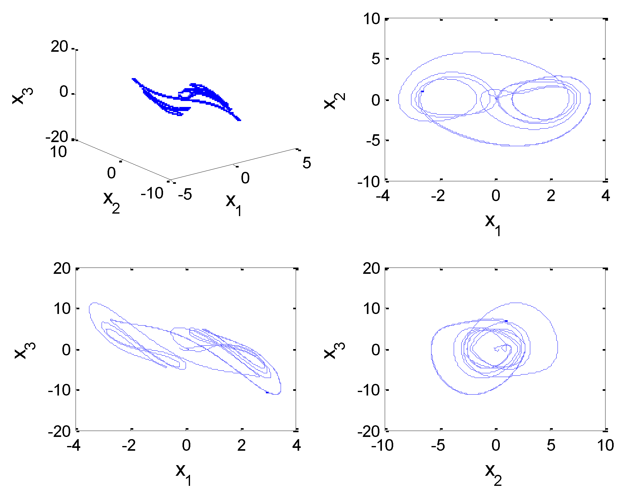
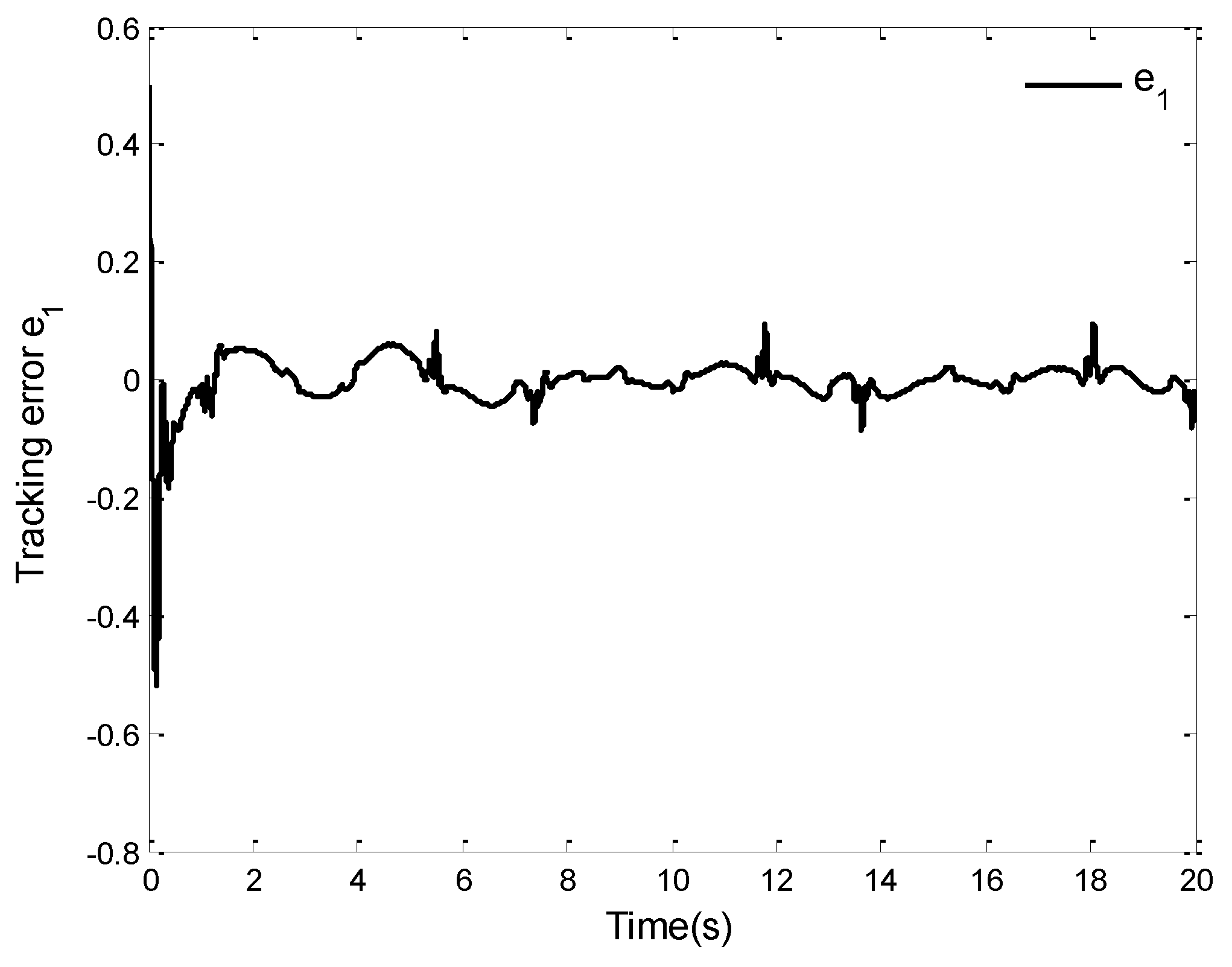
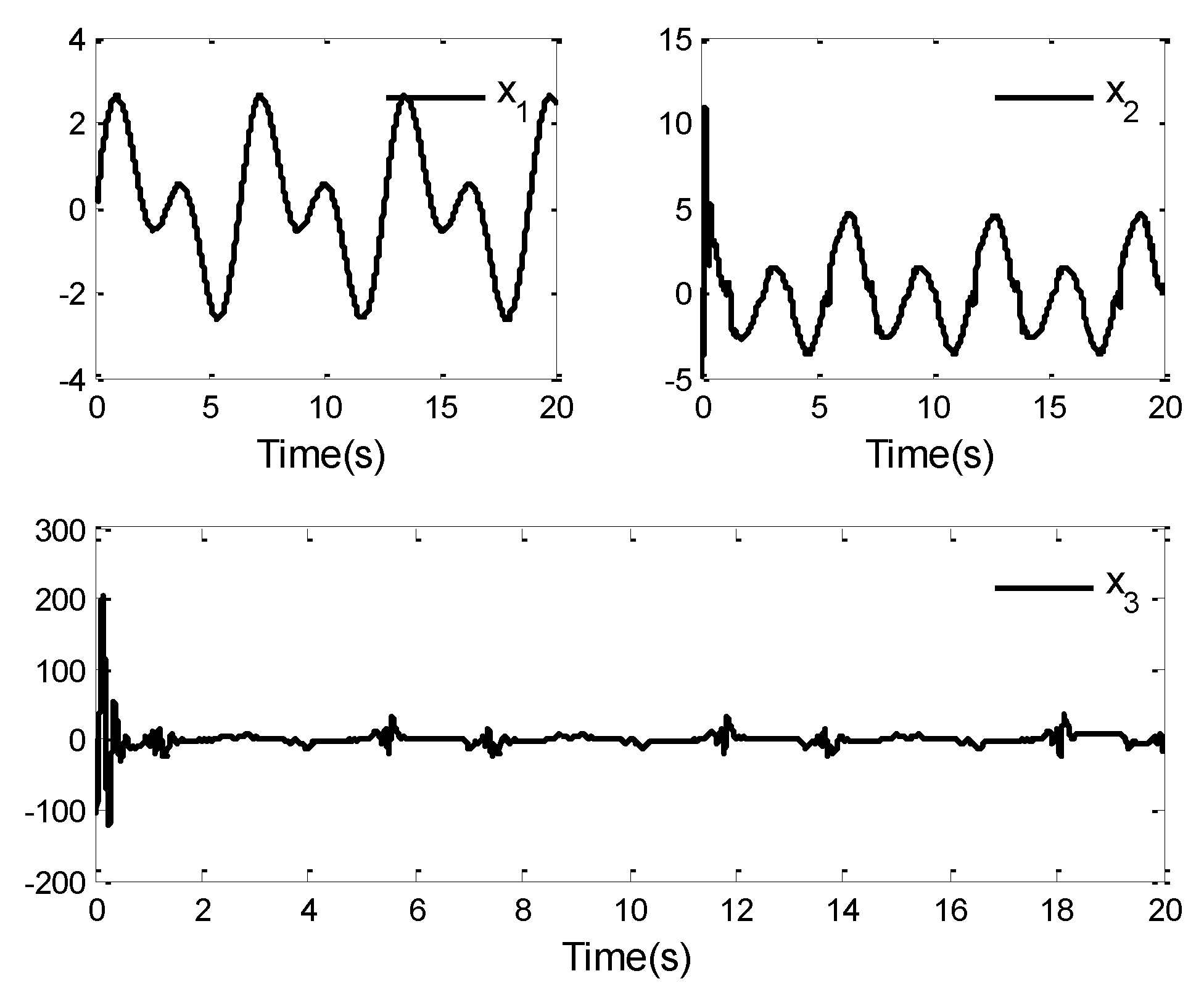
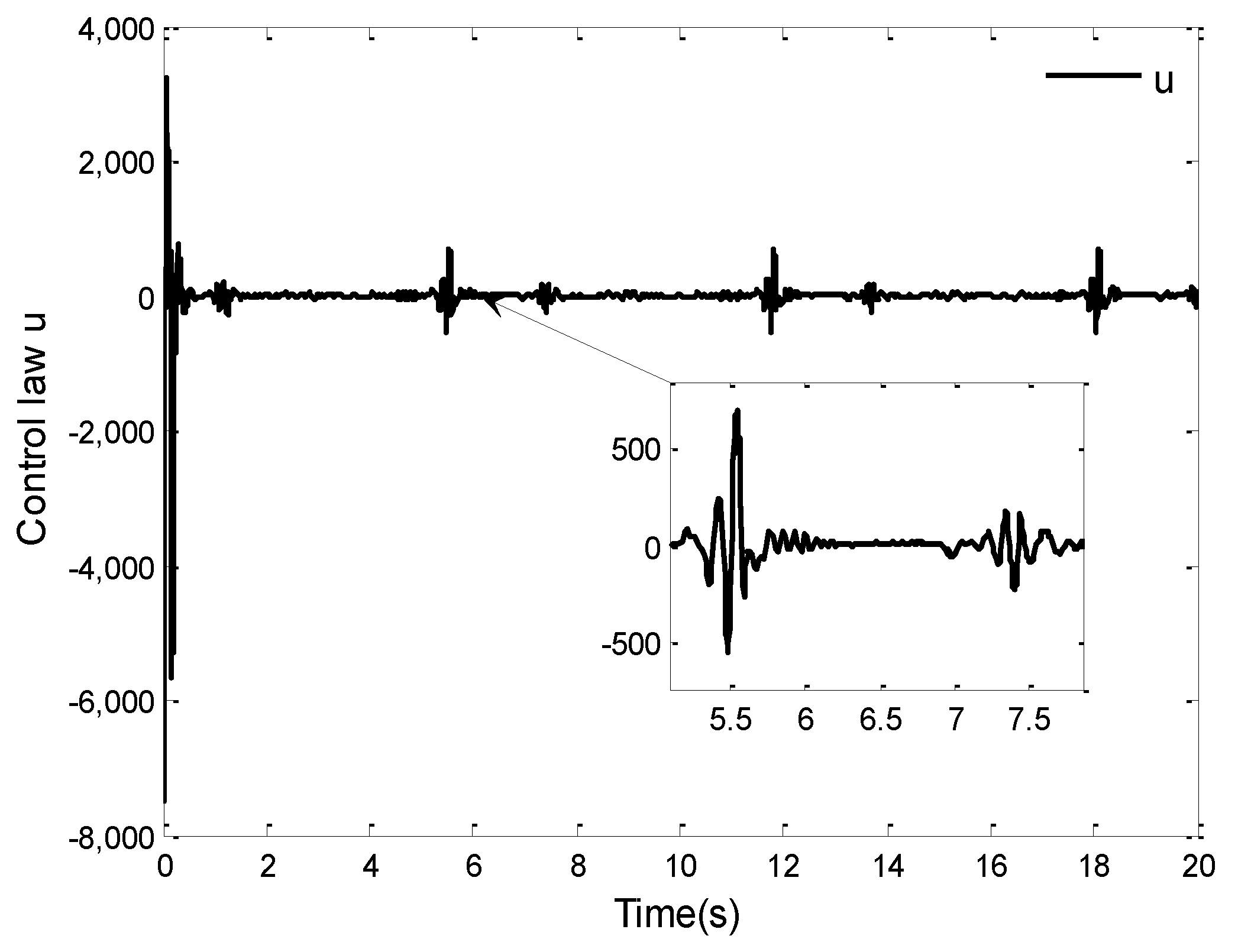
4. Simulation Analysis

In this section, the simulation cases are given to verify the validity of the control law designed in this paper.

Case 1: Consider a class of uncertain fractional-order systems as follows:

$$\begin{array}{l}{\mathcal{D}}_t^{\alpha }{x}_1=g_1{x}_2+f_1+{\mathit{\gamma }}_1^T{\mathit{\phi }}_1\\ {\mathcal{D}}_t^{\alpha }{x}_2=g_2{x}_3+f_2+{\mathit{\gamma }}_2^T{\mathit{\phi }}_2\\ {\mathcal{D}}_t^{\alpha }{x}_3=g_3{u}^F(t)+f_3+{\mathit{\gamma }}_3^T{\mathit{\phi }}_3\\ y=x_1\end{array}$$

(86)

where $g_1=0.9$, $g_2=0.5$, $g_3=1+0.7\sin t$, $f_1=-x_2\sin (x_1)$, $f_2=e^{-x_2^2/15}$, $f_3=2x_2-2x_3-\sin (x_1{x}_3)$, ${\mathit{\gamma }}_1={\mathit{\gamma }}_2={\mathit{\gamma }}_3={\left[0.5,1\right]}^T$, ${\mathit{\phi }}_1={\left[\cos (x_1),x_2\right]}^T$, ${\mathit{\phi }}_2={\left[-\sin (x_1{x}_2),-x_2\cos (x_3)\right]}^T$, and ${\mathit{\phi }}_3={\left[x_2,x_1^2\right]}^T$. The dead-zone fault model is shown in (2), and $k_d=1.5$, $b_l=0.15$ and $b_r=0.3$. The reference signal is $y_d=1.5\left(\sin t+\sin 2t\right)$; the initial states are $x_1(0)=1.2$, $x_2(0)=0.5$ and $x_3(0)=0.25$; and the simulation time is $t=20 \mathrm{s}$.

The RBFNN is used to approximate the unknown nonlinear functions $f_1$, $f_2$ and $f_3$. The node number for each RBF neural network is considered to be $9$ with the width of basis function being $\hslash =4$. The centers of the basis function ${\mathit{\iota }}_i$ ($i=1,\cdots ,9$) for the function $f_1$ are evenly spaced in $[-8,8]\times [-8,8]$; for the function $f_2$, they are evenly spaced in $[-8,8]$; and for the function $f_3$, they are evenly spaced in $[-8,8]\times [-8,8]\times [-8,8]$.

The other design parameters are $\vartheta =0.01$, $\beta =0.95$, ${\lambda }_1=1.5$, ${\lambda }_2=3.0$, ${\lambda }_3=4.5$, ${\ell }_1=1.5$, ${\ell }_2=2.0$, ${\ell }_3=0.5$, $c_1=20$, $c_2=12$, $c_3=2.0$, ${\mathrm{A}}_1=1.5$, ${\mathrm{A}}_2=2.5$, ${\mathrm{A}}_3=0.5$, ${\eta }_1=0.4$, ${\eta }_2=1.5$, ${\eta }_3=1.6$, ${\mathrm{B}}_1=4.5$, ${\mathrm{B}}_2=2.9$, ${\mathrm{B}}_3=1.5$, ${\delta }_1=0.5$, ${\delta }_2=3.0$, ${\delta }_3=5.5$, ${\epsilon }_1^{*}={\epsilon }_2^{*}=0.5$, ${\overline{\epsilon }}_3^{*}=1.0$. The parameters for the second-order command filter are set as $\omega =3.0$ and $\tau =0.7$. The initial conditions for adaptive laws are set as $s_1(0)=s_2(0)=s_3(0)=0.01$, ${\widehat{\mathit{\gamma }}}_1(0)={\widehat{\mathit{\gamma }}}_2(0)={\widehat{\mathit{\gamma }}}_3(0)={\left[0.01\right]}_{2\times 1}$, ${\widehat{\mathit{W}}}_1(0)={\widehat{\mathit{W}}}_2(0)={\widehat{\mathit{W}}}_3(0)={\left[0.01\right]}_{9\times 1}$ and $\kappa (0)=0$.

The simulation results for this case are shown in Figure 1, Figure 2, Figure 3, Figure 4, Figure 5 and Figure 6. Figure 1 and Figure 2 give the curves of the tracking performance and the tracking error $e_1$. It can be seen from Figure 1 that the system (86) can obtain a good tracking performance in finite time, although the system suffers from the unknown dead-zone fault. From Figure 2, we can see that the tracking error can converge to a small neighborhood of zero in finite time under the proposed control law. The results of these two figures also further verify the validity of the designed control law. Furthermore, the trajectories of the state variables $x_1$, $x_2$ and $x_3$ are displayed in Figure 3, the curves of the control law $u(t)$ and adaptive laws $‖{\widehat{\mathit{W}}}_i‖$ and $‖{\widehat{\mathit{\gamma }}}_i‖$ ($i=1,2,3$) are shown in Figure 4, Figure 5 and Figure 6. Noting Figure 2, Figure 3, Figure 4, Figure 5 and Figure 6, the signals of the closed-loop system are bounded in finite time, which shows the validity of the theoretical analysis.

Case 2: Consider the uncertain fractional-order Arneodo system as [49]

$$\begin{array}{l}{\mathcal{D}}_t^{\alpha }{x}_1=g_1{x}_2+f_1++{\mathit{\gamma }}_1^T{\mathit{\phi }}_1\\ {\mathcal{D}}_t^{\alpha }{x}_2=g_2{x}_3+f_2+{\mathit{\gamma }}_2^T{\mathit{\phi }}_2\\ {\mathcal{D}}_t^{\alpha }{x}_3=-q_1{x}_1-q_2{x}_2-q_3{x}_3-q_4{x}_1^3+g_3{u}^F(t)+f_3+{\mathit{\gamma }}_3^T{\mathit{\phi }}_3\\ y=x_1\end{array}$$

(87)

If $f_1=f_2=f_3=0$, ${\mathit{\gamma }}_1^T{\mathit{\phi }}_1={\mathit{\gamma }}_2^T{\mathit{\phi }}_2={\mathit{\gamma }}_3^T{\mathit{\phi }}_3=0$, $u^F(t)=0$ and $\alpha =0.98$, $g_1=g_2=1$, $q_1=-5.5$, $q_2=3.5$, $q_3=0.8$, $q_4=-1.0$, the initial conditions are considered to be $x_1(0)=-0.2$, $x_2(0)=0.5$, and $x_3(0)=0.2$. The system (87) will appear to have a chaotic phenomenon, as shown in Figure 7.

In system (87), let $g_3=1.2\sin x_1+2$, $f_1=-x_1{e}^{-10x_2}$, $f_2=-2.5x_2\cos x_3$, $f_3=-x_1\sin (x_3)$, ${\mathit{\gamma }}_1={\mathit{\gamma }}_2={\mathit{\gamma }}_3={\left[0.5,1\right]}^T$, ${\mathit{\phi }}_1={\left[-\sin x_1,0\right]}^T$, ${\mathit{\phi }}_2={\left[0,-\sin (x_1{x}_2)\right]}^T$, and ${\mathit{\phi }}_3={\left[3x_2,-2x_3\right]}^T$; the initial states are $x_1(0)=0.5$, $x_2(0)=0.25$ and $x_3(0)=0.1$. The parameters of the dead-zone fault model, the reference signal, and the simulation time are consistent with Case 1.

The RBF neural network is applied to approximate the unknown nonlinear functions $f_1$, $f_2$ and $f_3$. Since there are only two variables in functions $f_1$, $f_2$, and $f_3$, the node number for each RBF neural network is chosen to be $9$ with the centers of the basis function ${\mathit{\iota }}_i$ ($i=1,\cdots ,9$) evenly spaced in $[-8,8]\times [-8,8]$ and the width being $\hslash =4$.

The other design parameters are $\vartheta =0.01$, $\beta =0.95$, ${\lambda }_1=10$, ${\lambda }_2=5.5$, ${\lambda }_3=7.5$, ${\ell }_1=2.5$, ${\ell }_2=1.5$, ${\ell }_3=2.0$, $c_1=25$, $c_2=18$, $c_3=1.5$, ${\mathrm{A}}_1=0.9$, ${\mathrm{A}}_2=1.2$, ${\mathrm{A}}_3=0.2$, ${\eta }_1=0.5$, ${\eta }_2=2.5$, ${\eta }_3=3.0$, ${\mathrm{B}}_1=2.2$, ${\mathrm{B}}_2=1.6$, ${\mathrm{B}}_3=0.5$, ${\delta }_1=0.7$, ${\delta }_2=1.5$, ${\delta }_3=2.1$, ${\epsilon }_1^{*}=0.5$, ${\epsilon }_2^{*}=0.7$, and ${\overline{\epsilon }}_3^{*}=1.0$. The parameters selection of the second-order command filter and the initial conditions of the adaptive laws are the same as those described for Case 1.

The simulation results of this case are displayed in Figure 8, Figure 9, Figure 10, Figure 11, Figure 12 and Figure 13. Figure 8 shows the curves of the system output $x_1$ and the reference signal $y_d$. It is not difficult to see from Figure 8 that the system (87) can obtain a good tracking performance by applying the proposed control law. The tracking error curve is given in Figure 9. One observes that the tracking error $e_1$ can converge to a small neighborhood of zero in finite time. From Figure 8 and Figure 9, although the system (87) is affected by unknown dead zone fault, the tracking performance of the system can be guaranteed under the designed control law. This also proves the effectiveness of the proposed control law from another perspective. Furthermore, the curves of state variables $x_1$, $x_2$ and $x_3$ are given in Figure 10, and the curves of the control law $u(t)$ and adaptive laws $‖{\widehat{\mathit{W}}}_i‖$ and $‖{\widehat{\mathit{\gamma }}}_i‖$ ($i=1,2,3$) are depicted in Figure 11, Figure 12 and Figure 13. It can be found that the signals of the closed-loop system shown in these figures are bounded, which verifies the validity of the theoretical analysis. However, it is not difficult to observe in Figure 9, Figure 10 and Figure 11 that there are oscillations in these simulation results. In fact, considering the existence of unknown dead-zone faults and uncertain dynamics in the system, this makes it necessary to make a reasonable trade-off between system tracking performance and control output.

5. Conclusions

The adaptive finite-time tracking control for uncertain fractional-order systems with unknown dead-zone fault was considered in this paper. The fractional-order command filter was applied to avoid the computational complexity problem existing in conventional recursive procedures, and the neural network approximator was used to approximate the unknown uncertain nonlinear functions. Through the application of the Nussbaum gain function technique, the adaptive neural network finite-time control law was developed to solve the finite-time control problem of the given fractional-order systems. It has been proven that the desinged control law can not only ensure that all signals of the closed-loop system are bounded in finite time but can also ensure that the tracking error converges to a small neighborhood of the origin in finite time. However, it should be pointed out that the control law presented in this paper is only suitable for the systems with known state gains and measurable states. When the nonlinear system under consideration has unknown state gains and unmeasurable states, the proposed control law will not work effectively. Therefore, one of our future research directions is to design feasible control laws to realize the adaptive finite-time control of uncertain fractional-order systems with unknown control gain and partially unmeasurable states.

References

1. Li, Y.-X.; Yang, G.-H. Observer-based adaptive fuzzy quantized control of uncertain nonlinear systems with unknown control directions. Fuzzy Sets Syst. 2019, 371, 61–77. [Google Scholar] [CrossRef]
2. Zhao, X.; Wang, X.; Zhang, S.; Zong, G. Adaptive neural backstepping control design for a class of nonsmooth nonlinear systems. IEEE Trans. Syst. Man Cybern. Syst. 2019, 49, 1820–1831. [Google Scholar] [CrossRef]
3. Deng, X.; Zhang, C.; Ge, Y. Adaptive neural network dynamic surface control of uncertain strict-feedback nonlinear systems with unknown control direction and unknown actuator fault. J. Frankl. Inst. 2022, 359, 4054–4073. [Google Scholar] [CrossRef]
4. Kamalamiri, A.; Shahrokhi, M.; Mohit, M. Adaptive finite-time neural control of non-strict feedback systems subject to output constraint, unknown control direction, and input nonlinearities. Inf. Sci. 2020, 520, 271–291. [Google Scholar] [CrossRef]
5. Lai, G.; Liu, Z.; Zhang, Y.; Philip Chen, C.L.; Xie, S. Adaptive inversion-based fuzzy compensation control of uncertain pure-feedback systems with asymmetric actuator backlash. IEEE Trans. Fuzzy Syst. 2017, 25, 141–155. [Google Scholar] [CrossRef]
6. Yousefpour, A.; Jahanshahi, H.; Munoz-Pacheco, J.M.; Bekiros, S.; Wei, Z. A fractional-order hyper-chaotic economic system with transient chaos. Chaos Solitons Fractals 2022, 130, 109400. [Google Scholar] [CrossRef]
7. Monje, C.A.; Chen, Y.; Vinagre, B.M.; Xue, D.; Vicente, F. Fractional-Order Systems and Controls: Fundamentals and Applications; Springer: Berlin, Germany, 2010. [Google Scholar]
8. Demirci, E.; Ozalp, N. A method for solving differential equations of fractional-order. J. Comput. Appl. Math. 2012, 236, 2754–2762. [Google Scholar] [CrossRef]
9. Li, Y.; Chen, Y.; Podlubny, I. Mittag-leffler stability of fractional-order nonlinear dynamic systems. Automatica 2009, 45, 1965–1969. [Google Scholar] [CrossRef]
10. Li, C.; Deng, W. Remarks on fractional derivates. Appl. Math. Comput. 2007, 187, 777–784. [Google Scholar] [CrossRef]
11. Khamsuwan, P.; Kuntanapreeda, S. A linear matrix inequality approach to output feedback control of fractional-order unified chaotic systems with one control input. J. Comput. Nonlinear Dyn. 2016, 11, 051021. [Google Scholar] [CrossRef]
12. Zhao, Y.; Wang, Y.; Zhang, X.; Li, H. Feedback stabilisation control esign for fractional order non-linear systems in the lower triangular form. IET Control. Theory Appl. 2014, 8, 1238–1246. [Google Scholar]
13. Zhan, Y.; Sui, S.; Tong, S. Adaptive Fuzzy decentralized dynamic surface control for fractional-order nonlinear large-scale systems. IEEE Trans. Fuzzy Syst. 2022, 30, 3373–3383. [Google Scholar] [CrossRef]
14. Liang, B.; Zheng, S.; Ahn, C.K.; Liu, F. Adaptive fuzzy control for fractional-order interconnected systems with unknown control directions. IEEE Trans. Fuzzy Syst. 2022, 30, 75–87. [Google Scholar] [CrossRef]
15. Sui, S.; Chen, C.L.P.; Tong, S. Neural-network-based adaptive DSC design for switched fractional-order nonlinear systems. IEEE Trans. Neural Netw. Learn. Syst. 2021, 32, 4703–4712. [Google Scholar] [CrossRef] [PubMed]
16. Boulham, I.A.; Boubakir, A.; Labiod, S. Neural network L1 adaptive control for a class of uncertain fractional order nonlinear systems. Integration 2022, 83, 1–11. [Google Scholar] [CrossRef]
17. Li, R.; Zhang, X. Adaptive sliding mode observer design for a class of t–s fuzzy descriptor fractional order systems. IEEE Trans. Fuzzy Syst. 2020, 28, 1951–1960. [Google Scholar] [CrossRef]
18. Li, X.; Wen, C.; Zou, Y. Adaptive backstepping control for fractional-order nonlinear systems with external disturbance and uncertain parameters using smooth control. IEEE Trans. Syst. Man Cybern. Syst. 2021, 51, 7860–7869. [Google Scholar] [CrossRef]
19. Zirkohi, M.M. Robust adaptive backstepping control of uncertain fractional-order nonlinear systems with input time delay. Math. Comput. Simul. 2022, 196, 251–272. [Google Scholar] [CrossRef]
20. You, X.; Shi, M.; Guo, B.; Zhu, Y.; Lai, W.; Dian, S.; Liu, K. Event-triggered adaptive fuzzy tracking control for a class of fractional-order uncertain nonlinear systems with external disturbance. Chaos Solitons Fractals 2022, 161, 112393. [Google Scholar] [CrossRef]
21. Song, S.; Park, J.H.; Zhang, B.; Song, X. Observer-based adaptive hybrid fuzzy resilient control for fractional-order nonlinear systems with time-varying delays and actuator failures. IEEE Trans. Fuzzy Syst. 2021, 29, 471–485. [Google Scholar] [CrossRef]
22. Doostdar, F.; Mojallali, H. An ADRC-based backstepping control design for a class of fractional-order systems. ISA Trans. 2022, 121, 140–146. [Google Scholar] [CrossRef] [PubMed]
23. Yang, Z.; Zhang, H. A fuzzy adaptive tracking control for a class of uncertain strick-feedback nonlinear systems with dead-zone input. Neurocomputing 2018, 272, 130–135. [Google Scholar] [CrossRef]
24. Wu, L.-B.; Wang, H.; He, X.-Q.; Zhang, D.-Q. Decentralized adaptive fuzzy tracking control for a class of uncertain large-scale systems with actuator nonlinearities. Appl. Math. Comput. 2018, 332, 390–405. [Google Scholar] [CrossRef]
25. Zhang, C.-H.; Yang, G.-H. Event-triggered adaptive output feedback control for a class of uncertain nonlinear systems with actuator failures. IEEE Trans. Cybern. 2020, 50, 201–210. [Google Scholar] [CrossRef]
26. Yang, W.; Yu, W.; Zheng, W.X. Fault-tolerant adaptive fuzzy tracking control for nonaffine fractional-order full-state-constrained MISO systems with actuator failures. IEEE Trans. Cybern. 2022, 52, 8439–8452. [Google Scholar] [CrossRef]
27. Li, Y.-X.; Wang, Q.-Y.; Tong, S. Fuzzy adaptive fault-tolerant control of fractional-order nonlinear systems. IEEE Trans. Syst. Man Cybern. Syst. 2021, 51, 1372–1379. [Google Scholar] [CrossRef]
28. Wang, C.; Cui, L.; Liang, M.; Li, J.; Wang, Y. Adaptive neural network control for a class of fractional-order nonstrict-feedback nonlinear systems with full-state constraints and input saturation. IEEE Trans. Neural Netw. Learn. Syst. 2021. [Google Scholar] [CrossRef] [PubMed]
29. Liu, R.; Wang, Z.; Zhang, X.; Ren, J.; Gui, Q. Robust Control for Variable-Order Fractional Interval Systems Subject to Actuator Saturation. Fractal Fract. 2022, 6, 159. [Google Scholar] [CrossRef]
30. Zhan, Y.; Li, X.; Tong, S. Observer-Based Decentralized Control for Non-Strict-Feedback Fractional-Order Nonlinear Large-Scale Systems With Unknown Dead Zones. IEEE Trans. Neural Networks Learn. Syst. 2022. [Google Scholar] [CrossRef]
31. Nussbaum, R.D. Some remarks on a conjecture in parameter adaptive control. Syst. Control Lett. 1983, 3, 243–246. [Google Scholar] [CrossRef]
32. Oliveira, T.R.; Hsu, L.; Peixoto, A.J. Output-feedback global tracking for unknown control direction plants with application to extremum-seeking control. Automatica 2011, 47, 2029–2038. [Google Scholar] [CrossRef]
33. Lv, M.; Yu, W.; Cao, J.; Baldi, S. Consensus in High-Power Multiagent Systems With Mixed Unknown Control Directions via Hybrid Nussbaum-Based Control. IEEE Trans. Cybern. 2022, 52, 5184–5196. [Google Scholar] [CrossRef] [PubMed]
34. Lv, M.; De Schutter, B.; Shi, C.; Baldi, S. Logic-based distributed switching control for agents in power-chained form with multiple unknown control directions. Automatica 2022, 137, 110143. [Google Scholar] [CrossRef]
35. Cui, Q.; Huang, J.; Gao, T. Adaptive leaderless consensus control of uncertain multi-agent systems with unknown control directions. Int. J. Robust Nonlinear Control. 2020, 30, 6229–6240. [Google Scholar] [CrossRef]
36. Wang, K.; Liu, X.; Jing, Y. Adaptive finite-time command filtered controller design for nonlinear systems with output constraints and input nonlinearities. IEEE Trans. Neural Netw. Learn. Syst. 2021. [Google Scholar] [CrossRef]
37. Choi, Y.H.; Yoo, S.J. Quantized feedback adaptive command filtered backstepping control for a class of uncertain nonlinear strict-feedback systems. Nonlinear Dyn. 2020, 99, 2907–2918. [Google Scholar] [CrossRef]
38. Yu, J.; Shi, P.; Liu, J.; Lin, C. Neuroadaptive Finite-Time Control for Nonlinear MIMO Systems With Input Constraint. IEEE Trans. Cybern. 2022, 52, 6676–6683. [Google Scholar] [CrossRef]
39. Song, S.; Zhang, B.; Xia, J.; Zhang, Z. Adaptive Backstepping Hybrid Fuzzy Sliding Mode Control for Uncertain Fractional-Order Nonlinear Systems Based on Finite-Time Scheme. IEEE Trans. Syst. Man, Cybern. Syst. 2020, 50, 1559–1569. [Google Scholar] [CrossRef]
40. You, X.; Dian, S.; Liu, K.; Guo, B.; Xiang, G.; Zhu, Y. Command Filter-Based Adaptive Fuzzy Finite-Time Tracking Control for Uncertain Fractional-Order Nonlinear Systems. IEEE Trans. Fuzzy Syst. 2022. [Google Scholar] [CrossRef]
41. Li, Y.-X.; Wei, M.; Tong, S. Event-Triggered Adaptive Neural Control for Fractional-Order Nonlinear Systems Based on Finite-Time Scheme. IEEE Trans. Cybern. 2022, 52, 9481–9489. [Google Scholar] [CrossRef]
42. Wang, F.; Liu, Z.; Zhang, Y.; Chen, B. Distributed adaptive coordination control for uncertain nonlinear multi-agent systems with dead-zone input. J. Frankl. Inst. 2016, 353, 2270–2289. [Google Scholar] [CrossRef]
43. Podlubny, I. Fractional Differential Equations; Academic Press: New York, NY, USA, 1999. [Google Scholar]
44. Liu, H.; Pan, Y.; Li, S.; Chen, Y. Adaptive fuzzy backstepping control of fractional-order nonlinear systems. IEEE Trans. Syst. Man Cybern. Syst. 2017, 47, 2209–2217. [Google Scholar] [CrossRef]
45. Gong, P.; Lan, W. Adaptive Robust Tracking Control for Multiple Unknown Fractional-Order Nonlinear Systems. IEEE Trans. Cybern. 2019, 49, 1365–1376. [Google Scholar] [CrossRef] [PubMed]
46. Liu, Y.; Zhang, H.; Shi, Z.; Gao, Z. Neural-Network-Based Finite-Time Bipartite Containment Control for Fractional-Order Multi-Agent Systems. IEEE Trans. Neural Netw. Learn. Syst. 2022. [Google Scholar] [CrossRef] [PubMed]
47. Zhao, N.-N.; Ouyang, X.-Y.; Wu, L.-B.; Shi, F.-R. Event-triggered adaptive prescribed performance control of uncertain nonlinear systems with unknown control directions. ISA Trans. 2021, 108, 121–130. [Google Scholar] [CrossRef] [PubMed]
48. Alassafi, M.O.; Ha, S.; Alsaadi, F.E.; Ahmad, A.M.; Cao, J. Fuzzy synchronization of fractional-order chaotic systems using finite-time command filter. Inf. Sci. 2021, 579, 325–346. [Google Scholar] [CrossRef]
49. Ha, S.; Chen, L.; Liu, H.; Zhang, S. Command filtered adaptive fuzzy control of fractional-order nonlinear systems. Eur. J. Control 2022, 63, 48–60. [Google Scholar] [CrossRef]
Figure 1. Curves of tracking performance.
Fractalfract 06 00494 g001
Figure 2. Tracking error e 1 .
Fractalfract 06 00494 g002
Figure 3. System states x 1 , x 2 and x 3 .
Fractalfract 06 00494 g003
Figure 4. Control law u ( t ) .
Fractalfract 06 00494 g004
Figure 5. Norms of adaptive laws W ^ i .
Fractalfract 06 00494 g005
Figure 6. Norms of adaptive laws γ ^ i .
Fractalfract 06 00494 g006
Figure 7. Phrase plots of x 1 , x 2 , and x 3 .
Fractalfract 06 00494 g007
Figure 8. Curves of the tracking performance.
Fractalfract 06 00494 g008
Figure 9. Tracking error e 1 .
Fractalfract 06 00494 g009
Figure 10. System states x 1 , x 2 , and x 3 .
Fractalfract 06 00494 g010
Figure 11. Control law u ( t ) .
Fractalfract 06 00494 g011
Figure 12. Norms of adaptive laws W ^ i .
Fractalfract 06 00494 g012
Figure 13. Norms of adaptive laws γ ^ i .
Fractalfract 06 00494 g013
Publisher’s Note: MDPI stays neutral with regard to jurisdictional claims in published maps and institutional affiliations.