The Multicomponent Higher-Order Chen–Lee–Liu System: The Riemann–Hilbert Problem and Its N-Soliton Solution

Abstract

It is well known that multicomponent integrable systems provide a method for analyzing phenomena with numerous interactions, due to the interactions between their different components. In this paper, we derive the multicomponent higher-order Chen–Lee–Liu (mHOCLL) system through the zero-curvature equation and recursive operators. Then, we apply the trace identity to obtain the bi-Hamiltonian structure of mHOCLL system, which certifies that the constructed system is integrable. Considering the spectral problem of the Lax pair, a related Riemann–Hilbert (RH) problem of this integrable system is naturally constructed with zero background, and the symmetry of this spectral problem is given. On the one hand, the explicit expression for the mHOCLL solution is not available when the RH problem is regular. However, according to the formal solution obtained using the Plemelj formula, the long-time asymptotic state of the mHOCLL solution can be obtained. On the other hand, the N-soliton solutions can be explicitly gained when the scattering problem is reflectionless, and its long-time behavior can still be discussed. Finally, the determinant form of the N-soliton solution is given, and one-, two-, and three-soliton solutions as specific examples are shown via the figures.

1. Introduction

Many phenomena in natural science and engineering technology are nonlinear. These phenomena are complex and changeable, and cannot be described only with simple linear models. Therefore, nonlinear models can describe complex phenomena in daily life and scientific research more accurately than linear models, so as to reflect the nature of the relevant phenomena more accurately. As one type of nonlinear partial differential equations (nPDEs), the integrable equations have attracted more attention for their good properties [1,2,3]. In general, the integrable equations have their own Lax pair, Hamiltonian structure, and infinity symmetries. However, at the same time, it is very difficult to solve the exact solution of nPDEs due to the nonlinear term of the equation. In 1967, Gardner et al. proposed a new method for solving integrable equations—the inverse scattering method, which not only provided new concepts and methods for applied technology, but also had a profound impact on the development of mathematics [1]. The inverse scattering method uses the Lax pair of integrable systems and the spectral theory of ordinary differential equations to transform the Cauchy problem into a linear integral equation which can provide an explicit solution in the case of a degenerate kernel. However, when the kernel of the integral equation is non-degenerate, an explicit expression for the solution is hard to come by. In 1975, Shabat first used the RH method to study the spectral problem of integrable systems [4]. Compared with the classical inverse scattering method, the RH method has a wider application range, such as: for the second-order spectral problem, the generalized linear model (GLM) theory is equivalent to the RH method, but for the higher-order spectral problem, there is no GLM theory. Therefore, some parts of the inverse scattering problem need to be transformed into the RH problem. Most importantly, the long-time asymptotic properties of the non-soliton solution can be obtained by analyzing the RH problem [5]. Recently, scholars have studied the RH problem of many integrable equations, such as the Kundu–Eckhaus equation [6], the Wadati–Konno–Ichikawa equation [7], the derivative nonlinear Schrödinger equation [8], the quartic nonlinear Schrödinger equation [9], the vector modified Korteweg–de Vries equation [10], the focusing Hirota equation [11], and so on.

In particular, the nonlinear Schrödinger(NLS) equation and the derivative NLS equation are the most popular, and they are reduced from two different hierarchies, Ablowitz–Kaup–Newell–Sugar (AKNS) and Kaup–Newell (KN), respectively. The general formula of the derivative NLS equation can be written as [12]

$$\mathrm{i}{u}_t+u_{xx}+{\rho |u|}^{2}u+{\mathrm{i}a|u|}^2{u}_x+\mathrm{i}b{u}^2{u}_x^{*}+\frac{1}{4}b\left(2b-a\right){|u|}^{4}u=0,$$

(1)

which can be used to describe the propagation of short light pulses [13]. Equation (1) is reduced to the KN equation when $\rho =0,a=2b$ [14], Equation (1) changes into the CLL equation when $\rho =b=0$ [15,16], and Equation (1) changes into the Gerdjikov–Ivanov (GI) equation when $\rho =a=0$ [17,18]. As three types of derivative NLS, they can be changed with a gauge transformation, CLL → KN → GI. From a physical point of view, the GI equation has a high-order nonlinear term, while the KN equation has a self-dispersion term. From a mathematical point of view, these are three types of equations which have their unique Lax pairs. Up to now, there have some studies of these three equations, which mainly focus on the construction of the solution and the long-time asymptotic analysis.

In this paper, a mHOCLL equation is derived with a third-order dispersion and quintic nonlinear term:

$$\begin{array}{cc}\hfill u_{j,t_3}=& -u_{j,xxx}-{\displaystyle \frac{3\mathrm{i}}{2}}{|\mathit{u}|}^2{u}_{j,xx}-{\displaystyle \frac{3\mathrm{i}}{2}}{\mathit{u}}_x{\mathit{u}}^{*}{u}_{j,x}+{\displaystyle \frac{3}{4}}{|\mathit{u}|}^4{u}_{j,x},\hfill \end{array}$$

(2)

from a high-order hierarchy, where $1\le j\le n,\mathit{u}=\left(u_1,u_2,\cdots ,u_n\right),{\mathit{u}}^{*}={\left(u_1^{*},u_2^{*},\cdots ,u_n^{*}\right)}^{\mathrm{T}}$, and $*$ denotes the complex conjugate. When $n=1$, it is a scalar equation, whose Liouville integrability and multi-Hamiltonian structure have been given in [19]. Afterwards, its corresponding N-soliton was also obtained via the RH problem. Furthermore, the rogue wave and the N-soliton are constructed under the non-zero condition [15,16]. Compared to the general CLL, the high-order system behaves differently due to the effect of the high-order dispersion. More importantly, the multicomponent system produces richer characteristics between the different components. In recent years, multicomponent systems have received more and more attention [20,21,22,23]. Feng et al. studied the integrable semi-discretization of a multicomponent short pulse equation [20]. Gerdjikov et al. constructed the Jost solutions and the minimal set of scattering data for the case of local and non-local reductions [21]. Marvan et al. constructed a point transformation between two integrable systems, the multicomponent Harry Dym equation and the multicomponent extended Harry Dym equation, that does not preserve the class of multi-phase solutions [22]. Therefore, we intend to study the multicomponent equations as well as their Hamiltonian structure. Given this, the RH problem is constructed to obtain the N-order soliton.

In this paper, we mainly study the construction of the mHOCLL equation and obtain its soliton solution through a special correlated RH problem. According to the RH method, there are generally two standard steps required to solve nPDEs [24,25,26,27]. One is that nPDEs be transformed into the RH problem on the complex plane; that is, nPDEs must be raised to the complex plane for consideration. The other one is that the unsolvable RH problem be transformed into a solvable RH problem by decomposing the jump matrix, the deformation integral path, etc.

This paper is structured as follows. Section 2 constructs the mHOCLL integrable system and its bi-Hamiltonian structure. Section 3 studies the analytical properties of the Jost solution and builds the RH problem associated with the mHOCLL system. Section 4 gives the formal solution when the RH problem is regular and the N-soliton solution when there is no reflection coefficient, and discusses its long-time asymptotic state. Then, the determinant form of the N-soliton solution is given and one-, two-, and three-soliton solutions as specific examples are shown via the figures. Section 5 is the conclusion.

2. Multicomponent Higher-Order Chen–Lee–Liu Integrable Hierarchies

The Lax pair of the scalar CLL system is well known and has been well studied, but the mHOCLL system is rarely studied. Therefore, in this section, we build a mHOCLL system and its bi-Hamiltonian structure which certifies that the constructed system is integrable.

Firstly, we extend the scalar potential to the vector potential and introduce a spectral problem as follows:

$${\psi }_x=\mathcal{M}\psi =\mathcal{M}(\mathit{u},{\mathit{u}}^{*},\lambda )\psi ,$$

(3)

where $\mathcal{M}=\left[\begin{array}{cc}-\mathrm{i}{\lambda }^2& \lambda \mathit{u}\\ -\lambda {\mathit{u}}^{*}& \mathrm{i}{\lambda }^2{I}_n-{\displaystyle \frac{1}{2}}\mathrm{i}{\mathit{u}}^{*}\mathit{u}\end{array}\right],$$\lambda$ denotes the spectral parameter, and $\mathit{u}$ is defined in Equation (2).

Then, a solution $\mathcal{N}$ is considered as

$$\mathcal{N}=\left[\begin{array}{cc}A& \mathit{B}\\ \mathit{C}& \mathit{D}\end{array}\right],$$

(4)

where A is a scalar, ${\mathit{B}}^{\mathrm{T}}$, $\mathit{C}$ are two n-dimensional columns, $\mathit{D}$ is an $n\times n$ matrix, and ${}^{\mathrm{T}}$ denotes matrix the transpose. Based on Equation (A2), we can obtain

$$\left\{\begin{array}{cc}\hfill & A_x=\lambda \mathit{u}\mathit{C}+\lambda \mathit{B}{\mathit{u}}^{*},\hfill \\ \hfill & {\mathit{B}}_x=\lambda \mathit{u}\mathit{D}-\lambda A\mathit{u}-2\mathrm{i}{\lambda }^2\mathit{B}+{\displaystyle \frac{\mathrm{i}}{2}}\mathit{B}{\mathit{u}}^{*}\mathit{u},\hfill \\ \hfill & {\mathit{C}}_x=\lambda \mathit{D}{\mathit{u}}^{*}-\lambda {\mathit{u}}^{*}A+2\mathrm{i}{\lambda }^2\mathit{C}-{\displaystyle \frac{\mathrm{i}}{2}}{\mathit{u}}^{*}\mathit{u}\mathit{C},\hfill \\ \hfill & {\mathit{D}}_x=-\lambda {\mathit{u}}^{*}\mathit{B}-\lambda \mathit{C}\mathit{u}+{\displaystyle \frac{\mathrm{i}}{2}}(\mathit{D}{\mathit{u}}^{*}\mathit{u}-{\mathit{u}}^{*}\mathit{u}\mathit{D}).\hfill \end{array}\right.$$

(5)

Then, $\mathcal{N}$ is written in the following form:

$$\mathcal{N}={\displaystyle \sum _{m=0}^{\infty }}{\mathcal{N}}_m{\lambda }^{-m}, m\ge 0,$$

(6)

where

$${\mathcal{N}}_m=\left[\begin{array}{cc}{A}^{[m]}& {\mathit{B}}^{[m]}\\ {\mathit{C}}^{[m]}& {\mathit{D}}^{[m]}\end{array}\right],{\mathit{B}}^{[m]}=(B_1^{[m]},\dots ,B_n^{[m]}),{\mathit{C}}^{[m]}={(C_1^{[m]},\dots ,C_n^{[m]})}^{\mathrm{T}},{\mathit{D}}^{[m]}={(D_{ij}^{[m]})}_{n\times n},$$

(7)

Then, we can obtain four recursion relations:

$$A^{[2m+1]}=0, {\mathit{B}}^{[2m]}=\mathbf{0}, {\mathit{C}}^{[2m]}=\mathbf{0}, {\mathit{D}}^{[2m+1]}=\mathbf{0}, A_x^{[0]}=0, {\mathit{D}}_x^{[0]}=\mathbf{0},$$

(8a)

$$A_x^{[2m]}=\mathit{u}{\mathit{C}}^{[2m+1]}+{\mathit{B}}^{[2m+1]}{\mathit{u}}^{*},$$

(8b)

$${\mathit{B}}^{[2m+1]}=\frac{\mathrm{i}}{2}(A^{[2m]}\mathit{u}-\mathit{u}{\mathit{D}}^{[2m]}+{\mathit{B}}_x^{[2m-1]}-\frac{\mathrm{i}}{2}{\mathit{B}}^{[2m-1]}{\mathit{u}}^{*}\mathit{u}),$$

(8c)

$${\mathit{C}}^{[2m+1]}=\frac{\mathrm{i}}{2}({\mathit{D}}^{[2m]}{\mathit{u}}^{*}-{\mathit{u}}^{*}{A}^{[2m]}-{\mathit{C}}_x^{[2m-1]}-\frac{\mathrm{i}}{2}{\mathit{u}}^{*}\mathit{u}{\mathit{C}}^{[2m-1]}),$$

(8d)

$$D_x^{[2m]}=-{\mathit{C}}^{[2m+1]}\mathit{u}-{\mathit{u}}^{*}{\mathit{B}}^{[2m+1]}+\frac{\mathrm{i}}{2}({\mathit{D}}^{[2m]}{\mathit{u}}^{*}\mathit{u}-{\mathit{u}}^{*}\mathit{u}{\mathit{D}}^{[2m]}), m\ge 1.$$

(8e)

To obtain the mHOCLL system, we take a specific set of initial values

$$A^{[0]}=-4\mathrm{i}, {\mathit{D}}^{[0]}=4\mathrm{i}{I}_n, {\mathit{B}}^{[1]}=4\mathit{u}, {\mathit{C}}^{[1]}=-4{\mathit{u}}^{*}.$$

(9)

Then, we can obtain

$$A^{[2]}=2\mathrm{i}\mathit{u}{\mathit{u}}^{*}, {\mathit{D}}^{[2]}=-2\mathrm{i}{\mathit{u}}^{*}\mathit{u}, {\mathit{B}}^{[3]}=2\mathrm{i}{\mathit{u}}_x-\mathit{u}{\mathit{u}}^{*}\mathit{u}, {\mathit{C}}^{[3]}=2\mathrm{i}{\mathit{u}}_x^{*}+{\mathit{u}}^{*}\mathit{u}{\mathit{u}}^{*},$$

(10a)

$$A^{[4]}=\mathit{u}{\mathit{u}}_x^{*}-{\mathit{u}}_x{\mathit{u}}^{*}-\frac{\mathrm{i}}{2}\mathit{u}{\mathit{u}}^{*}\mathit{u}{\mathit{u}}^{*},{\mathit{D}}^{[4]}-{\mathit{u}}_x^{*}\mathit{u}+{\mathit{u}}^{*}{\mathit{u}}_x+\frac{\mathrm{i}}{2}{\mathit{u}}^{*}\mathit{u}{\mathit{u}}^{*}\mathit{u},$$

(10b)

$${\mathit{B}}^{[5]}=-{\mathit{u}}_{xx}+\frac{\mathrm{i}}{2}\mathit{u}{\mathit{u}}_x^{*}\mathit{u}-\frac{\mathrm{i}}{2}{\mathit{u}}_x{\mathit{u}}^{*}\mathit{u}-\mathrm{i}{\mathit{u}\mathit{u}}^{*}{\mathit{u}}_x+\frac{1}{4}\mathit{u}{\mathit{u}}^{*}\mathit{u}{\mathit{u}}^{*}\mathit{u},$$

(10c)

$${\mathit{C}}^{[5]}={\mathit{u}}_{xx}^{*}+\frac{\mathrm{i}}{2}{\mathit{u}}^{*}{\mathit{u}}_x{\mathit{u}}^{*}-\mathrm{i}{\mathit{u}}_x^{*}\mathit{u}{\mathit{u}}^{*}-\frac{\mathrm{i}}{2}{\mathit{u}}^{*}\mathit{u}{\mathit{u}}_x^{*}-\frac{1}{4}{\mathit{u}}^{*}\mathit{u}{\mathit{u}}^{*}\mathit{u}{\mathit{u}}^{*},$$

(10d)

$$\begin{array}{cc}\hfill A^{[6]}& =-\frac{\mathrm{i}}{2}\mathit{u}{\mathit{u}}_{xx}^{*}-\frac{\mathrm{i}}{2}{\mathit{u}}_{xx}{\mathit{u}}^{*}+\frac{\mathrm{i}}{2}{\mathit{u}}_x{\mathit{u}}_x^{*}-\frac{1}{4}\mathit{u}{\mathit{u}}_x^{*}\mathit{u}{\mathit{u}}^{*}-\frac{1}{2}\mathit{u}{\mathit{u}}^{*}\mathit{u}{\mathit{u}}_x^{*}+\frac{1}{2}{\mathit{u}}_x{\mathit{u}}^{*}\mathit{u}{\mathit{u}}^{*}\hfill \\ & +\frac{1}{4}\mathit{u}{\mathit{u}}^{*}{\mathit{u}}_x{\mathit{u}}^{*},\hfill \end{array}$$

(10e)

$$\begin{array}{cc}\hfill {\mathit{D}}^{[6]}& =\frac{\mathrm{i}}{2}{\mathit{u}}_{xx}^{*}\mathit{u}+\frac{\mathrm{i}}{2}{\mathit{u}}^{*}{\mathit{u}}_{xx}-\frac{\mathrm{i}}{2}{\mathit{u}}_x^{*}{\mathit{u}}_x-\frac{1}{4}{\mathit{u}}^{*}{\mathit{u}}_x{\mathit{u}}^{*}\mathit{u}-\frac{1}{2}{\mathit{u}}^{*}\mathit{u}{\mathit{u}}^{*}{\mathit{u}}_x+\frac{1}{2}{\mathit{u}}_x^{*}\mathit{u}{\mathit{u}}^{*}\mathit{u}\hfill \\ & +\frac{1}{4}{\mathit{u}}^{*}\mathit{u}{\mathit{u}}_x^{*}\mathit{u}-\frac{\mathrm{i}}{8}{\mathit{u}}^{*}\mathit{u}{\mathit{u}}^{*}\mathit{u}{\mathit{u}}^{*}\mathit{u},\hfill \\ & ⋮\end{array}$$

(10f)

Meanwhile, according to the recursion relations (8), we can know

$$\left[\begin{array}{c}{\mathit{B}}^{[2m+1]\top }\\ {\mathit{C}}^{[2m+1]}\end{array}\right]=R_2{R}_1\left[\begin{array}{c}{\mathit{B}}^{[2m-1]\top }\\ {\mathit{C}}^{[2m-1]}\end{array}\right], m\ge 1,$$

(11)

where

$$\begin{array}{cc}\hfill R_1& ={\displaystyle \frac{1}{4}}\left[\begin{array}{cc}-\partial I_n+{\displaystyle \frac{\mathrm{i}}{2}}{\mathit{u}}^{\mathrm{T}}{\mathit{u}}^{*\mathrm{T}}& 0\\ 0& \partial I_n+{\displaystyle \frac{\mathrm{i}}{2}}{\mathit{u}}^{*}\mathit{u}\end{array}\right],\hfill \\ \hfill R_2& =\left[\begin{array}{cc}{\mathit{u}}^{*}{\partial }^{-1}\mathit{u}+{\displaystyle \sum _{j=1}^n}{u}_j^{*}{\partial }^{-1}{u}_j-2\mathrm{i}{I}_n& {\mathit{u}}^{\mathrm{T}}{\partial }^{-1}\mathit{u}+{({\mathit{u}}^{\mathrm{T}}{\partial }^{-1}\mathit{u})}^{\mathrm{T}}\\ -{\mathit{u}}^{*}{\partial }^{-1}{\mathit{u}}^{*\mathrm{T}}-{({\mathit{u}}^{*}{\partial }^{-1}{\mathit{u}}^{*\mathrm{T}})}^{\mathrm{T}}& -{\mathit{u}}^{\mathrm{T}}{\partial }^{-1}{\mathit{u}}^{*\mathrm{T}}-{\displaystyle \sum _{j=1}^n}{u}_j{\partial }^{-1}{u}_j^{*}-2\mathrm{i}{I}_n\end{array}\right].\hfill \end{array}$$

(12)

Secondly, the Lax matrix is rewritten as

$$\begin{array}{cc}\hfill {\mathcal{N}}^{[\tilde{n}]}& ={({\lambda }^{\tilde{n}}\mathcal{N})}_{+}+{▵}_{\tilde{n}}\hfill \\ & =\sum _{m=0}^{\tilde{n}-1}\left[\begin{array}{cc}{A}^{[2m+2]}{\lambda }^{2(\tilde{n}-m)}+A^{[0]}{\lambda }^{2\tilde{n}}& {\mathit{B}}^{[2m+1]}{\lambda }^{2(\tilde{n}-m)-1}\\ {\mathit{C}}^{[2m+1]}{\lambda }^{2(\tilde{n}-m)-1}& {\mathit{D}}^{[2m+2]}{\lambda }^{2(\tilde{n}-m)}+{\mathit{D}}^{[0]}{\lambda }^{2\tilde{n}}\end{array}\right]+\left[\begin{array}{cc}{\Delta }_{\tilde{n}}& 0\\ 0& {\nabla }_{\tilde{n}}\end{array}\right],\tilde{n}\ge 1,\hfill \end{array}$$

(13)

where the subscript ${}_{+}$ represents the positive part of the polynomial with respect to $\lambda$, and ${▵}_{\tilde{n}}$ is the modification term. Then, according to the compatibility condition, we gain ${\Delta }_{\tilde{n}}=-\frac{1}{2}{\partial }^{-1}({\mathit{B}}^{[2\tilde{n}+1]}{\mathit{u}}^{*}+\mathit{u}{\mathit{C}}^{[2\tilde{n}+1]})$ and ${\nabla }_{\tilde{n}}=\frac{1}{2}{\partial }^{-1}({\mathit{u}}^{*}{\mathit{B}}^{[2\tilde{n}+1]}+{\mathit{C}}^{[2\tilde{n}+1]}\mathit{u})$. Then, the mHOCLL hierarchies are gained using the zero-curvature equation, Equation (A4) in Appendix A:

$${\mathbf{F}}_{t_{\tilde{n}}}:={\left[\begin{array}{c}{\mathit{u}}^{\mathrm{T}}\\ {\mathit{u}}^{*}\end{array}\right]}_{t_{\tilde{n}}}=K_{\tilde{n}}=\left[\begin{array}{c}-2\mathrm{i}{\mathit{B}}^{[2\tilde{n}+1]\mathrm{T}}+{\mathit{u}}^{\mathrm{T}}{\Delta }_{\tilde{n}}^{\mathrm{T}}-{\nabla }_{\tilde{n}}^{\mathrm{T}}{\mathit{u}}^{\mathrm{T}}\\ -2\mathrm{i}{\mathit{C}}^{[2\tilde{n}+1]}+{\nabla }_{\tilde{n}}{\mathit{u}}^{*}-{\mathit{u}}^{*}{\Delta }_{\tilde{n}}\end{array}\right]=R_3{R}_1\left[\begin{array}{c}{\mathit{B}}^{[2\tilde{n}+1]\mathrm{T}}\\ {\mathit{C}}^{[2\tilde{n}+1]}\end{array}\right], \tilde{n}\ge 1,$$

(14)

where $R_3=\left[\begin{array}{cc}1& R_{31}\\ R_{32}& I_n\end{array}\right]$ with

$$\begin{array}{cc}\hfill R_{31}& ={\displaystyle \frac{3}{2}}({\mathit{u}}^{*}{\partial }^{-1}\mathit{u}+\sum _{j=1}^n{u}_j^{*}{\partial }^{-1}{u}_j){(-{\mathit{u}}^{*}{\partial }^{-1}{\mathit{u}}^{*\mathrm{T}}-{({\mathit{u}}^{*}{\partial }^{-1}{\mathit{u}}^{*\mathrm{T}})}^{\mathrm{T}})}^{-1},\hfill \\ \hfill R_{32}& ={\displaystyle \frac{3}{2}}(-{\mathit{u}}^{\mathrm{T}}{\partial }^{-1}{\mathit{u}}^{*\mathrm{T}}-\sum _{j=1}^n{u}_j{\partial }^{-1}{u}_j^{*}){({\mathit{u}}^{\mathrm{T}}{\partial }^{-1}\mathit{u}+{({\mathit{u}}^{\mathrm{T}}{\partial }^{-1}\mathit{u})}^{\mathrm{T}})}^{-1}.\hfill \end{array}$$

When $\tilde{n}=3$, the mHOCLL hierarchy is transformed into the mHOCLL equation:

$$\begin{array}{cc}\hfill u_{j,t_3}=& -u_{j,xxx}-{\displaystyle \frac{3\mathrm{i}}{2}}{|\mathit{u}|}^2{u}_{j,xx}-{\displaystyle \frac{3\mathrm{i}}{2}}{\mathit{u}}_x{\mathit{u}}^{*}{u}_{j,x}+{\displaystyle \frac{3}{4}}{|\mathit{u}|}^4{u}_{j,x}, 1\le j\le n,\hfill \end{array}$$

(15)

which can be reduced to the higher-order CLL equation as $n=1$.

Then, we determine the Liouville integrability of the mHOCLL hierarchies (14) using bi-Hamiltonian structures which are presented by the trace identity or the variational identity [28,29,30]. It is easy to gain from the matrix $\mathcal{M}$ and $\mathcal{N}$

$$\mathrm{tr}(\mathcal{N}\frac{\partial \mathcal{M}}{\partial \lambda })=-2\mathrm{i}\lambda A-\mathit{B}\mathit{u}*+\mathrm{tr}(\mathit{C}\mathit{u}+2\mathrm{i}\lambda D),$$

(16a)

$$\mathrm{tr}(\mathcal{N}\frac{\partial \mathcal{M}}{\partial \mathit{u}})=\lambda \mathit{C}-\frac{1}{2}\mathrm{i}\mathit{D}\mathit{u}*,$$

(16b)

$$\mathrm{tr}(\mathcal{N}\frac{\partial \mathcal{M}}{\partial {\mathit{u}}^{*}})=-\lambda \mathit{B}-\mathrm{i}\mathit{u}\mathit{D}.$$

(16c)

According to the trace identity (A8), we have

$${\displaystyle \frac{\delta }{\delta \mathit{F}}}(-2\mathrm{i}\lambda A-\mathit{B}{\mathit{u}}^{*}+\mathrm{tr}(\mathit{C}\mathit{u}+2\mathrm{i}\lambda \mathit{D}))={\lambda }^{-\gamma }{\displaystyle \frac{\partial }{\partial \lambda }}[{\lambda }^{\gamma }(\lambda \mathit{C}-{\displaystyle \frac{1}{2}}\mathrm{i}\mathit{D}{\mathit{u}}^{*},-\lambda \mathit{B}-{\displaystyle \frac{1}{2}}\mathrm{i}\mathit{u}\mathit{D})].$$

(17)

Substituting

$$A=\sum _{\tilde{n}\ge 0}{A}^{[2\tilde{n}]}{\lambda }^{-2\tilde{n}},\mathit{B}=\sum _{\tilde{n}\ge 0}{\mathit{B}}^{[2\tilde{n}+1]}{\lambda }^{-2\tilde{n}-1},\mathit{C}=\sum _{\tilde{n}\ge 0}{\mathit{C}}^{[2\tilde{n}+1]}{\lambda }^{-2\tilde{n}-1},\mathit{D}=\sum _{\tilde{n}\ge 0}{\mathit{D}}^{[2\tilde{n}]}{\lambda }^{-2\tilde{n}}$$

into Equation (17) yields

$${\displaystyle \frac{\delta }{\delta \mathit{F}}}(-2\mathrm{i}{A}^{[2\tilde{n}+2]}-{\mathit{B}}^{[2\tilde{n}+1]}{\mathit{u}}^{*}+\sum _{i=1}^n{({\mathit{C}}^{[2\tilde{n}+1]}\mathit{u}+2\mathrm{i}{\mathit{D}}^{[2\tilde{n}+2]})}_{ii})=(-2\tilde{n}-\gamma )G_{2\tilde{n}+1}.$$

(18)

Plugging these into the trace identity, we find that $\gamma =0$, and thereby it is easy to have

$${\displaystyle \frac{\delta {\tilde{H}}_{\tilde{n}}}{\delta \mathit{F}}}=G_{2\tilde{n}+1},$$

(19)

where

$$\begin{array}{cc}\hfill & {\tilde{H}}_{\tilde{n}}={\displaystyle \frac{1}{2\tilde{n}}}(2\mathrm{i}{A}^{[2\tilde{n}+2]}+{\mathit{B}}^{[2\tilde{n}+1]}{\mathit{u}}^{*}-\sum _{i=1}^n{({\mathit{C}}^{[2\tilde{n}+1]}\mathit{u}+2\mathrm{i}{\mathit{D}}^{[2\tilde{n}+2]})}_{ii}),\hfill \\ \hfill & G_{2\tilde{n}+1}=\left[\begin{array}{c}{\mathit{B}}^{[2\tilde{n}+1]\mathrm{T}}\\ {\mathit{C}}^{[2\tilde{n}+1]}\end{array}\right], \tilde{n}\ge 1.\hfill \end{array}$$

(20)

Then, we obtain the bi-Hamiltonian structure of the mHOCLL system:

$${\mathit{F}}_{t_{\tilde{n}}}=L_1{\displaystyle \frac{\delta {\tilde{H}}_{\tilde{n}}}{\delta \mathit{F}}}=L_2{\displaystyle \frac{\delta {\tilde{H}}_{\tilde{n}-1}}{\delta \mathit{F}}}, \tilde{n}\ge 1,$$

(21)

where the Hamiltonian pairs $L_1=R_3{R}_1,L_2=R_3{R}_1{R}_2{R}_1$.

Thus, each of the operators $L_1^{-1}{L}_2$ with a fixed $\tilde{n}$ is a recursion operator of per integrable hierarchy. Adjoint symmetry constraints decompose each mHOCLL system into two commuting finite-dimensional Liouville integrable Hamiltonian systems [29,31].

3. Riemann–Hilbert Problem

In this section, we construct the RH problem of the mHOCLL system, acquire the symmetries of some matrices, and discuss the time evolution of the time-dependent scattering coefficients.

Firstly, the Lax pairs of the mHOCLL system need to be rewritten as

$${\psi }_x=\mathcal{M}(\mathit{F},\lambda )\psi ,$$

(22)

$${\psi }_{t_{\tilde{n}}}={\mathcal{N}}^{[\tilde{n}]}(\mathit{F},\lambda )\psi ,$$

(23)

with

$$\mathcal{M}=\mathrm{i}{\lambda }^2\Lambda +\widehat{Q}(\mathit{F},\lambda ),{\mathcal{N}}^{[\tilde{n}]}=4\mathrm{i}{\lambda }^{2\tilde{n}}\Lambda +{\widehat{Y}}^{[\tilde{n}]}(\mathit{F},\lambda ), \tilde{n}\ge 1,$$

where

$$\widehat{Q}=\left[\begin{array}{cc}0& 0\\ 0& {\displaystyle \frac{\mathrm{i}}{2}}{\mathit{u}}^{*}\mathit{u}\end{array}\right]+\lambda Q_1,{\mathcal{N}}^{[\tilde{n}]}=\sum _{m=1}^{\tilde{n}}\left[\begin{array}{cc}{A}^{[2m]}{\lambda }^{2(\tilde{n}-m)}+{\Delta }_{\tilde{n}}& {\mathit{B}}^{[2m-1]}{\lambda }^{2(\tilde{n}-m)+1}\\ {\mathit{C}}^{[2m-1]}{\lambda }^{2(\tilde{n}-m)+1}& {\mathit{D}}^{[2m]}{\lambda }^{2(\tilde{n}-m)}+{\nabla }_{\tilde{n}}\end{array}\right].$$

(24)

Here, $Q_1=\left[\begin{array}{cc}0& \mathit{u}\\ -{\mathit{u}}^{*}& 0\end{array}\right],\Lambda =\mathrm{diag}(-1,I_n)$, $A^{[m]},{\mathit{B}}^{[m]},{\mathit{C}}^{[m]},{\mathit{D}}^{[m]}$ are defined in Equation (7) and $\mathit{F}$ is defined in Equation (14). We can easily find that the tr$(\widehat{Q})\ne 0$, and thus we need an appropriate transformation to make tr$(\widehat{Q})=0$. Let us take a kind of gauge transformation

$$\tilde{\psi }=(exp(-\mathrm{i}{\int }_{-\infty }^x{|\mathit{u}|}^2(y,t){\tilde{\Lambda }}_1\mathrm{d}y)+{\tilde{\Lambda }}_2)\psi , \tilde{\mathit{u}}=\mathit{u}exp({\displaystyle \frac{\mathrm{i}}{2}}{\int }_{-\infty }^x{|\mathit{u}|}^2(y,t)\mathrm{d}y),$$

(25)

where ${\tilde{\Lambda }}_1=\mathrm{diag}(-{\displaystyle \frac{1}{2}},0\ast I_n),{\tilde{\Lambda }}_2=\mathrm{diag}(0,I_n)$ and $|\tilde{\mathit{u}}|=|\mathit{u}|$. Then, Equations (22) and (23) are transformed into

$${\tilde{\psi }}_x=\tilde{\mathcal{M}}(\tilde{\mathit{F}},\lambda )\psi ,$$

(26)

$${\tilde{\psi }}_{t_{\tilde{n}}}={\tilde{\mathcal{N}}}^{[\tilde{n}]}(\tilde{\mathit{F}},\lambda )\psi ,$$

(27)

with

$$\tilde{\mathcal{M}}=\mathrm{i}{\lambda }^2\Lambda +\tilde{Q}(\tilde{\mathit{F}},\lambda ),{\tilde{\mathcal{N}}}^{[\tilde{n}]}=4\mathrm{i}{\lambda }^{2\tilde{n}}\Lambda +{\tilde{Y}}^{[\tilde{n}]}(\tilde{\mathit{F}},\lambda ),\tilde{n}\ge 1,$$

where

$$\tilde{Q}=\left[\begin{array}{cc}{\displaystyle \frac{\mathrm{i}}{2}}\tilde{\mathit{u}}{\tilde{\mathit{u}}}^{*}& 0\\ 0& -{\displaystyle \frac{\mathrm{i}}{2}}{\tilde{\mathit{u}}}^{*}\tilde{\mathit{u}}\end{array}\right]+\lambda {\tilde{Q}}_1,{\tilde{\mathcal{N}}}^{[\tilde{n}]}=\sum _{m=1}^{\tilde{n}}\left[\begin{array}{cc}{A}^{[2m]}{\lambda }^{2(\tilde{n}-m)}+{\Delta }_{\tilde{n}}& {\tilde{\mathit{B}}}^{[2m-1]}{\lambda }^{2(\tilde{n}-m)+1}\\ {\tilde{\mathit{C}}}^{[2m-1]}{\lambda }^{2(\tilde{n}-m)+1}& {\mathit{D}}^{[2m]}{\lambda }^{2(\tilde{n}-m)}+{\nabla }_{\tilde{n}}\end{array}\right].$$

(28)

Here,

$${\tilde{Q}}_1=\left[\begin{array}{cc}0& \tilde{\mathit{u}}\\ -{\tilde{\mathit{u}}}^{*}& 0\end{array}\right],{\tilde{\mathit{B}}}^{[m]}={\mathit{B}}^{[m]}exp({\displaystyle \frac{\mathrm{i}}{2}}{\int }_{-\infty }^x{|\mathit{u}|}^2(y,t)\mathrm{d}y),{\tilde{\mathit{C}}}^{[m]}={\mathit{C}}^{[m]}exp({\displaystyle \frac{\mathrm{i}}{2}}{\int }_{-\infty }^x{|\mathit{u}|}^2(y,t)\mathrm{d}y).$$

When all the potentials rapidly vanish as $x,t\to \pm \infty$, the asymptotic behavior is easy to obtain from Equations (26) and (27): $\tilde{\psi }\sim {\mathrm{e}}^{\mathrm{i}{\lambda }^2\Lambda x+4\mathrm{i}{\lambda }^{2\tilde{n}}\Lambda t_{\tilde{n}}}$. Then, we introduce a new function

$$\widehat{\varphi }=\tilde{\psi }{\mathrm{e}}^{-\mathrm{i}{\lambda }^2\Lambda x-4\mathrm{i}{\lambda }^{2\tilde{n}}\Lambda t_{\tilde{n}}},$$

(29)

which satisfies the canonical normalization $\widehat{\varphi }\to I_{n+1}$, when $x,t\to \pm \infty$. Substituting Equation (29) into Equations (22) and (23), it is easy to obtain

$${\widehat{\varphi }}_x=\mathrm{i}{\lambda }^2[\Lambda ,\widehat{\varphi }]+\tilde{Q}\widehat{\varphi },$$

(30)

$${\widehat{\varphi }}_{t_{\tilde{n}}}=4\mathrm{i}{\lambda }^{2\tilde{n}}[\Lambda ,\widehat{\varphi }]+{\tilde{Y}}^{[\tilde{n}]}\widehat{\varphi }.$$

(31)

Consider a solution to Equations (36) and (37) of the form

$$\widehat{\varphi }=D+{\displaystyle \frac{{\widehat{\varphi }}_1}{\lambda }}+{\displaystyle \frac{{\widehat{\varphi }}_2}{{\lambda }^2}}+{\displaystyle \frac{{\widehat{\varphi }}_3}{{\lambda }^3}}+\mathrm{O}({\displaystyle \frac{1}{{\lambda }^4}})$$

(32)

where D and $\widehat{\varphi }(k=1,2,3)$ are independent of the spectral parameter $\lambda$. Substituting Equation (32) into Equations (36) and (37) and comparing the same order of $\lambda$, it is easy to know that D is diagonal and satisfies

$$D_x={\displaystyle \frac{\mathrm{i}}{2}}{\tilde{Q}}_1^2\Lambda D,$$

(33)

$$D_t=\left[\begin{array}{cc}{A}^{[2\tilde{n}]}+{\Delta }_{\tilde{n}}& 0\\ 0& {\mathit{D}}^{[2\tilde{n}]}+{\nabla }_{\tilde{n}}\end{array}\right]D,$$

(34)

According to the $\tilde{\mathcal{M}}$, ${\tilde{\mathcal{N}}}^{[\tilde{n}]}$ and Equation (A4), we can know

$${({\displaystyle \frac{\mathrm{i}}{2}}{\tilde{Q}}_1^2\Lambda )}_t={\left[\begin{array}{cc}{A}^{[2\tilde{n}]}+{\Delta }_{\tilde{n}}& 0\\ 0& {\mathit{D}}^{[2\tilde{n}]}+{\nabla }_{\tilde{n}}\end{array}\right]}_x.$$

Therefore, we can define D as

$$D=exp({\int }_{-\infty }^x{\displaystyle \frac{\mathrm{i}}{2}}{\tilde{Q}}_1^2(y,t)\Lambda \mathrm{d}y),$$

(35)

and then we introduce a new function $\varphi$ which satisfies $D\varphi =\widehat{\varphi }$. Based on the asymptotic behavior of $\widehat{\varphi }$, it is evident that

$$\varphi =I_{n+1}+\mathrm{O}({\displaystyle \frac{1}{\lambda }}).$$

Then, we can obtain from Equations (30) and (31)

$${\varphi }_x=\mathrm{i}{\lambda }^2[\Lambda ,\widehat{\varphi }]+Q\widehat{\varphi },$$

(36)

$${\varphi }_{t_{\tilde{n}}}=4\mathrm{i}{\lambda }^{2\tilde{n}}[\Lambda ,\widehat{\varphi }]+Y^{[\tilde{n}]}\widehat{\varphi },$$

(37)

where

$$\begin{array}{cc}\hfill & Q=exp(-{\int }_{-\infty }^x{\displaystyle \frac{\mathrm{i}}{2}}{\tilde{Q}}_1^2(y,t)\Lambda \mathrm{d}y)\tilde{Q}exp({\int }_{-\infty }^x{\displaystyle \frac{\mathrm{i}}{2}}{\tilde{Q}}_1^2(y,t)\Lambda \mathrm{d}y),\hfill \\ \hfill & Y^{[\tilde{n}]}=exp(-{\int }_{-\infty }^x{\displaystyle \frac{\mathrm{i}}{2}}{\tilde{Q}}_1^2(y,t)\Lambda \mathrm{d}y){\tilde{Y}}^{[\tilde{n}]}exp({\int }_{-\infty }^x{\displaystyle \frac{\mathrm{i}}{2}}{\tilde{Q}}_1^2(y,t)\Lambda \mathrm{d}y).\hfill \end{array}$$

The Jost solutions ${\varphi }^{\pm }$ obey the constant asymptotic condition

$${\varphi }^{\pm }\to {\varphi }_0^{\pm },$$

(38)

when $x\to \pm \infty$, respectively.

Based on the boundary conditions (38) and the method of variation of the parameters, Equation (36) can be transformed into the Volterra integral equations [5] as follows:

$${\varphi }^{\pm }(\lambda ,x)={\varphi }_0^{\pm }+{\int }_{\pm \infty }^x{\mathrm{e}}^{\mathrm{i}{\lambda }^2\Lambda (x-y)}Q(y){\varphi }^{\pm }(\lambda ,y){\mathrm{e}}^{\mathrm{i}{\lambda }^2\Lambda (y-x)}\mathrm{d}y,$$

(39)

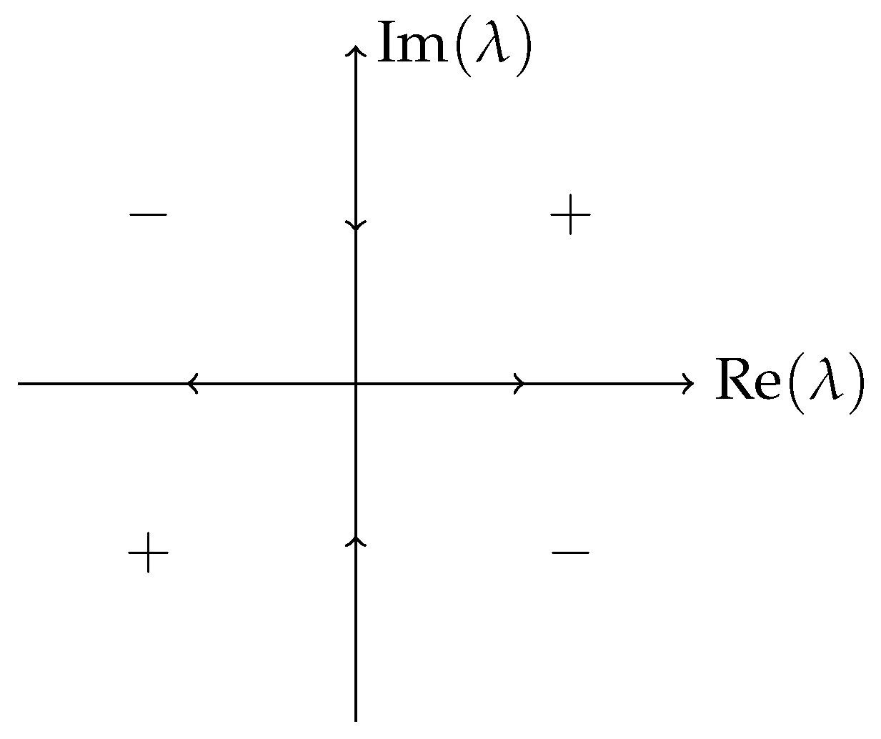
where ${\varphi }_0^{-}=I_{n+1}$ and ${\varphi }_0^{+}=exp(-{\int }_{-\infty }^{\infty }{\displaystyle \frac{\mathrm{i}}{2}}\tilde{Q}{(y,t)}_1^2\Lambda \mathrm{d}y).$ From Equation (39), it is evident that the first column of ${\varphi }^{-}$ involves only the exponential factor ${\mathrm{e}}^{2\mathrm{i}{\lambda }^2(x-y)}$. When $\lambda$ is in ${\Gamma }_{+}=\{\lambda \in \mathbb{C}|arg\lambda \in (0,\frac{\pi }{2})\bigcup (\pi ,\frac{3\pi }{2})\}$, the first column of ${\varphi }^{-}$ decays because of $y<x$, and allows for analytical continuations to ${\Gamma }_0=\{\mathbb{R}\bigcup \mathrm{i}\mathbb{R}\}$. Meanwhile, the last n columns of ${\varphi }^{+}$ involve only the exponential factor ${\mathrm{e}}^{-2\mathrm{i}{\lambda }^2(x-y)}$. Therefore, when $\lambda$ is in ${\Gamma }_{+}=\{\lambda \in \mathbb{C}|arg\lambda \in (0,\frac{\pi }{2})\bigcup (\pi ,\frac{3\pi }{2})\}$, they decay because of $y>x$, and this allows for analytical continuations to the real and imaginary axis. Similarly, it is obvious that the last n columns of ${\varphi }^{-}$ and the first column of ${\varphi }^{+}$ are analytical in ${\Gamma }_{-}=\{\lambda \in \mathbb{C}|arg\lambda \in (\frac{\pi }{2},\pi )\bigcup (\frac{3\pi }{2},2\pi )\}$ and analytically continued to ${\Gamma }_0$ (see Figure 1).

There is a linear relationship with matrix $S(\lambda )$

$${\varphi }^{-}E={\varphi }^{+}ES(\lambda ), \lambda \in {\Gamma }_0,$$

(40)

because

$${\psi }^{\pm }={\varphi }^{\pm }E,$$

(41)

are they are both solutions of Equation (22). Here, $E={\mathrm{e}}^{\mathrm{i}{\lambda }^2\Lambda x},$$S(\lambda )={(s_{ij})}_{(n+1)\times (n+1)}$ is the scattering matrix and satisfies det $S(\lambda )=1$, and

$$S(\lambda )=\underset{x\to +\infty }{lim}{E}^{-1}{\varphi }^{-}E=I+{\int }_{-\infty }^{+\infty }{\mathrm{e}}^{-\mathrm{i}{\lambda }^2\Lambda y}Q(y){\varphi }^{-}(\lambda ,y){\mathrm{e}}^{\mathrm{i}{\lambda }^2\Lambda y}\mathrm{d}y,\lambda \in {\Gamma }_0.$$

It is easy to know that $s_{11}$ allows for analytic extension to ${\Gamma }_{+}$, and $s_{ij}(i,j=2,\cdots ,n+1)$ are analytically extended to ${\Gamma }_{-}$.

Then, we build two matrix eigenfunctions ${\mathcal{K}}^{\pm }(x,\lambda )$ and make them continue analytically to ${\Gamma }_{+}$ and ${\Gamma }_{-}$, respectively. We define ${\varphi }^{\pm }$ as

$${\varphi }^{\pm }=({\varphi }_1^{\pm },{\varphi }_2^{\pm },\cdots ,{\varphi }_{n+1}^{\pm }).$$

(42)

Then, according to the analyticity of ${\varphi }^{\pm }$, we obtain

$${\mathcal{K}}^{+}={\mathcal{K}}^{+}(x,\lambda )=({\varphi }_1^{-},{\varphi }_2^{+},\cdots ,{\varphi }_{n+1}^{+})={\varphi }^{-}{T}_1+{\varphi }^{+}{T}_2$$

(43)

where $T_1$ and $T_2$ are defined by

$$T_1=\mathrm{diag}(1,\underset{n}{\underbrace{0,\cdots ,0}}),T_2=\mathrm{diag}(0,\underset{n}{\underbrace{1,\cdots ,1}}).$$

(44)

${\mathcal{K}}^{+}$ is analytic in ${\Gamma }_{+}$ and continuous to ${\Gamma }_0$. Substituting ${\mathcal{K}}^{+}$ into Equation (40), it is evident that

$${\mathcal{K}}^{+}={\varphi }^{+}E{S}^{+}{E}^{-1}={\varphi }^{+}E\left[\begin{array}{cccc}{s}_{11}& 0& \cdots & 0\\ s_{21}& 1& \cdots & 0\\ ⋮& ⋮& \ddots & ⋮\\ s_{n+1,1}& 0& \cdots & 1\end{array}\right]E^{-1}$$

Then, $det({\mathcal{K}}^{+})=s_{11}.$

The matrix eigenfunction which is analytic in ${\Gamma }_{+}$ has been constructed above. Now, we build the matrix eigenfunction which is analytic in ${\Gamma }_{-}$, which need the adjoint matrix spectral problems

$${\tilde{\varphi }}_x=-\mathrm{i}{\lambda }^2[\tilde{\varphi },\Lambda ]-\tilde{\varphi }Q.$$

(45)

Due to det ${\varphi }^{\pm }=1$, the adjoint matrix ${\tilde{\varphi }}^{\pm }={({\varphi }^{\pm })}^{-1}$. Similarly, we define ${\tilde{\varphi }}^{\pm }$ as

$${\tilde{\varphi }}^{\pm }={({\tilde{\varphi }}_1^{\pm },{\tilde{\varphi }}_2^{\pm },\cdots ,{\tilde{\varphi }}_{n+1}^{\pm })}^{\mathrm{T}}.$$

(46)

Then, the corresponding matrix eigenfunction ${\mathcal{K}}^{-}$ is written as

$${\mathcal{K}}^{-}={({\tilde{\varphi }}_1^{-},{\tilde{\varphi }}_2^{+},\cdots ,{\tilde{\varphi }}_{n+1}^{+})}^{\mathrm{T}}=T_1{\tilde{\varphi }}^{-}+T_2{\tilde{\varphi }}^{+},$$

(47)

and

$${\mathcal{K}}^{-}=E{S}^{-1}{E}^{-1}{({\varphi }^{+})}^{-1}=E\left[\begin{array}{cccc}{\widehat{s}}_{11}& {\widehat{s}}_{12}& \cdots & {\widehat{s}}_{1,n+1}\\ 0& 1& \cdots & 0\\ ⋮& ⋮& \ddots & ⋮\\ 0& 0& \cdots & 1\end{array}\right]E^{-1}{({\varphi }^{+})}^{-1}.$$

Here, $S^{-1}(\lambda ):={({\widehat{s}}_{ij})}_{(n+1)\times (n+1)}$, det$({\mathcal{K}}^{-})={\widehat{s}}_{11}$, and ${\mathcal{K}}^{-}$ is analytic in ${\Gamma }_{-}$ and continuous to ${\Gamma }_0$.

According to the matrix functions ${\mathcal{K}}^{\pm }$, it is easy to obtain from Equations (40), (43), and (47)

$${\mathcal{K}}^{+}(x,\lambda )={\mathcal{K}}^{-}(x,\lambda )J(x,\lambda ), \lambda \in {\Gamma }_0,$$

(48)

where

$$\begin{array}{cc}\hfill J(x,\lambda )& =E(T_1+T_{2}S(\lambda ))(T_1+S^{-1}(\lambda )T_2)E^{-1}\hfill \\ \hfill & =E\left[\begin{array}{ccccc}1& {\widehat{s}}_{12}& {\widehat{s}}_{13}& \cdots & {\widehat{s}}_{1,n+1}\\ s_{21}& 1& 0& \cdots & 0\\ s_{31}& 0& 1& \cdots & 0\\ ⋮& ⋮& ⋮& \ddots & ⋮\\ s_{n+1,1}& 0& 0& \cdots & 1\end{array}\right]E^{-1}.\hfill \end{array}$$

(49)

Then, the generalized RH problem for the mHOCLL systems is expressed as

$$\begin{array}{cc}\hfill & \star \mathcal{K}(x,t,\lambda )\mathrm{is}\mathrm{meromorphic}\mathrm{in}\mathbb{C}\backslash {\Gamma }_0,\hfill \\ \hfill & \star {\mathcal{K}}^{+}(x,\lambda )={\mathcal{K}}^{-}(x,\lambda )J(x,\lambda ), \lambda \in {\Gamma }_0,\hfill \\ \hfill & \star {\mathcal{K}}^{\pm }=I+O({\displaystyle \frac{1}{\lambda }}),\lambda \to \infty ,\hfill \end{array}$$

(50)

where ${\Gamma }_0$ denotes the jump contour.

Secondly, the symmetries of some matrices are considered. Due to $Q^{†}({\lambda }^{*})=-Q(\lambda )$, we can obtain the Hermitian equation of Equation (36):

$${\varphi }_x^{†}({\lambda }^{*})=-\mathrm{i}{\lambda }^2[{\varphi }^{†}({\lambda }^{*}),\Lambda ]-{\varphi }^{†}({\lambda }^{*})Q(\lambda ),$$

(51)

where ${}^{†}$ denotes the conjugate transpose. Combine Equations (45) and (51), and the properties of differential equations, and it is obvious that the involution relation is

$${\varphi }^{†}({\lambda }^{*})={\varphi }^{-1}(\lambda ).$$

Then, we obtain the involution property of $S(\lambda )$ through Equation (40):

$$S^{†}({\lambda }^{*})=S^{-1}(\lambda ).$$

(52)

The similar analysis shows that the Jost solutions the satisfy symmetry relation

$$\varphi (-\lambda )={\sigma }_3\varphi (\lambda ){\sigma }_3,$$

where ${\sigma }_3=\mathrm{diag}(1,\underset{n}{\underbrace{-1,\cdots ,-1}}).$ Then, it is easy to obtain

$$S(-\lambda )={\sigma }_{3}S(\lambda ){\sigma }_3,$$

(53)

Next, we study the properties of $s_{11}$ and ${\widehat{s}}_{11}$, which play an important role in a later analysis. From Equations (52) and (53), we obtain the following relations:

$$s_{11}^{*}({\lambda }^{*})={\widehat{s}}_{11}(\lambda )$$

(54)

and

$$s_{11}(\lambda )=s_{11}(-\lambda ).$$

(55)

Based on the symmetry relation, we can know that if $\lambda \in {\Gamma }_{+}$ is a zero of $s_{11}$, $-\lambda$ is another zero of $s_{11}$. According to the involution relation, it is visible that ${\widehat{s}}_{11}$ has two zeros, namely, $\pm {\lambda }^{*}$.

Next, substituting Equation (41) into Equation (37), we obtain

$$S_{t_{\tilde{n}}}=4\mathrm{i}{\lambda }^{2\tilde{n}}[\Lambda ,S].$$

(56)

The evolution of the time part of the scattering coefficient is expressed by

$$s_{1,j}=s_{1,j}(\lambda ,0){\mathrm{e}}^{8\mathrm{i}{\lambda }^{2\tilde{n}}{t}_{\tilde{n}}}, s_{i,1}=s_{i,1}(\lambda ,0){\mathrm{e}}^{-8\mathrm{i}{\lambda }^{2\tilde{n}}{t}_{\tilde{n}}}, 2\le i,j\le n+1,$$

(57)

and all other scattering coefficients are independent of the time variable $t_{\tilde{n}}$.

4. Solutions with the Riemann–Hilbert Method

In this section, we use the RH method to obtain the solutions to the mHOCLL system. There are two cases of the RH problem. One is the regular RH problem; the other is the non-regular RH problem.

Firstly, when the RH problem is regular, i.e., $det{\mathcal{K}}^{+}=s_{11}\ne 0$ and $det{\mathcal{K}}^{-}={\widehat{s}}_{11}\ne 0$, the explicit expression for the mHOCLL solution is not available, but we can obtain the formal solution obtained with the Plemelj formula. ${\Phi }^{\pm }={\mathcal{K}}_0^{-1}{\mathcal{K}}^{\pm }$ are introduced and used to rewrite the RH problem with the boundary condition

$${({\Phi }^{-})}^{-1}{\Phi }^{+}=J, \lambda \in {\Gamma }_0,$$

(58)

and

$${\Phi }^{\pm }\to I_{n+1},$$

(59)

when $\lambda \to \infty$. Then, according to Equation (48) and the Plemelj formula, we obtain

$${({\Phi }^{+})}^{-1}=I_{n+1}+{\displaystyle \frac{1}{2\pi \mathrm{i}}}{\int }_{\widehat{\Gamma }}{\displaystyle \frac{\widehat{J}(\zeta ){({\Phi }^{+})}^{-1}(\zeta )}{\zeta -\lambda }}\mathrm{d}\zeta , \lambda \in {\Gamma }_{+},$$

where $\widehat{J}=J-I_{n+1}$ and $\widehat{\Gamma }=[0,\infty )\cup (\mathrm{i}\infty ,0]\cup [0,-\infty )\cup (-\mathrm{i}\infty ,0]$.

Suppose that ${\widehat{\Phi }}^{\pm }$ and ${\Phi }^{\pm }$ are two sets of solutions to Equation (58); then, ${({\Phi }^{-})}^{-1}{\Phi }^{+}={({\widehat{\Phi }}^{-})}^{-1}{\widehat{\Phi }}^{+}$, namely,

$${\Phi }^{+}{({\widehat{\Phi }}^{+})}^{-1}={\Phi }^{-}{({\widehat{\Phi }}^{-})}^{-1},\lambda \in {\Gamma }_0.$$

(60)

If ${\Phi }^{+}{({\widehat{\Phi }}^{+})}^{-1}$ and ${\Phi }^{-}{({\widehat{\Phi }}^{-})}^{-1}$ are analytic in ${\Gamma }_{+}$ and ${\Gamma }_{-}$, respectively, a matrix function in the whole plane is defined by virtue of analytic continuation. According to Equation (59), this analytic function approaches the unit matrix $I_{n+1}$ when $\lambda \to \infty$. In complex analysis, Liouville’s theorem tells that if a function is analytic and bounded in the entire complex plane, then this function must be a constant. Then, based on this theorem, it is easy to know that

$${\Phi }^{+}{({\widehat{\Phi }}^{+})}^{-1}={\Phi }^{-}{({\widehat{\Phi }}^{-})}^{-1}=I_{n+1}$$

in the whole plane. Thus, ${\widehat{\Phi }}^{\pm }={\Phi }^{\pm }$, which indicates that the solution is unique.

Secondly, we discuss the soliton solution for the RH problem with $det{\mathcal{K}}^{+}=0$ and $det{\mathcal{K}}^{-}=0$. The uniqueness of the solutions to each associated RH problem (48) does not hold unless the zeros of det ${\mathcal{K}}^{\pm }$ in ${\Gamma }_{\pm }$ are specified, and the structures of ker ${\mathcal{K}}^{\pm }$ at those zeros are determined in [32,33,34].

From Equations (40), (43) and (47) it is visible that

$$\det {\mathcal{K}}^{+}(x,\lambda )=s_{11}(\lambda ),\det {\mathcal{K}}^{-}(x,\lambda )={\widehat{s}}_{11}(\lambda ).$$

(61)

According to the symmetry and involution relations of $s_{11}$ and ${\widehat{s}}_{11}$, we suppose that $s_{11}$ has $2N$ zeros $\{\pm {\lambda }_k\in {\Gamma }_{+},1\le k\le N\}$, and ${\widehat{s}}_{11}$ has $2N$ zeros $\{\pm {\widehat{\lambda }}_k\in {\Gamma }_{-},1\le k\le N\}$. Here, we only discuss the case of a single zero; that is, all zeros $\pm {\lambda }_k$ and $\pm {\widehat{\lambda }}_k$ are simple. In this case, each of ker ${\mathcal{K}}^{+}(x,{\lambda }_k)$ and ker ${\mathcal{K}}^{-}(x,{\widehat{\lambda }}_k)$ only contain a single basis column vector and row vector, respectively. Then, it is easy to know that

$${\mathcal{K}}^{+}(x,{\lambda }_k){\mathit{g}}_k=0, {\widehat{\mathit{g}}}_k{\mathcal{K}}^{-}(x,{\widehat{\lambda }}_k)=0, 1\le k\le N.$$

(62)

According to [35,36,37], we know that the RH problem, which has the canonical normalization condition and zero structures in Equation (62), can be solved. When $J=I_{n+1}$, we obtain $s_{i,1}={\widehat{s}}_{1,j}=0(2\le i,j\le n+1)$; that is, no reflection exists in the scattering problem. The solutions to this RH problem can be expressed as

$$\begin{array}{cc}\hfill & {\mathcal{K}}^{+}(x,\lambda )=I_{n+1}-\sum _{k,l=1}^N({\displaystyle \frac{{\mathit{g}}_k{({{\rm Y}}^{-1})}_{kl}{\widehat{\mathit{g}}}_l}{\lambda -{\widehat{\lambda }}_l}}-{\displaystyle \frac{{\sigma }_3{\mathit{g}}_k{({{\rm Y}}^{-1})}_{kl}{\widehat{\mathit{g}}}_l{\sigma }_3}{\lambda +{\widehat{\lambda }}_l}}),\hfill \\ \hfill & {\mathcal{K}}^{-}(x,\lambda )=I_{n+1}-\sum _{k,l=1}^N({\displaystyle \frac{{\widehat{\mathit{g}}}_l^{†}{({{\rm Y}}^{-1})}_{kl}^{†}{\mathit{g}}_k^{†}}{\lambda -{\lambda }_l}}-{\displaystyle \frac{{\sigma }_3{\widehat{\mathit{g}}}_l^{†}{({{\rm Y}}^{-1})}_{kl}^{†}{\mathit{g}}_k^{†}{\sigma }_3}{\lambda +{\lambda }_l}}),\hfill \end{array}$$

(63)

where

$${\rm Y}:={({\upsilon }_{kl})}_{N\times N},1\le k,l\le N,$$

(64)

with ${\upsilon }_{kl}={\displaystyle \frac{{\widehat{\mathit{g}}}_k{\mathit{g}}_l}{{\lambda }_l-{\widehat{\lambda }}_k}}-{\displaystyle \frac{{\widehat{\mathit{g}}}_k{\sigma }_3{\mathit{g}}_l}{{\lambda }_l+{\widehat{\lambda }}_k}}$. Because the space part and time part are independent, we can easily obtain from Equation (36) and Equation (62)

$${\mathcal{K}}^{+}(x,{\lambda }_k)({\displaystyle \frac{\mathrm{d}{\mathit{g}}_k}{\mathrm{d}x}}-\mathrm{i}{\lambda }_k^2\Lambda {\mathit{g}}_k)=0,1\le k\le N.$$

(65)

If we combine this with Equation (62), we know that the vectors ${\displaystyle \frac{\mathrm{d}{\mathit{g}}_k}{\mathrm{d}x}}-\mathrm{i}{\lambda }_k^2\Lambda {\mathit{g}}_k$ and ${\mathit{g}}_k$ have a linear relationship. Without loss of generality, we take the simplest case

$${\displaystyle \frac{\mathrm{d}{\mathit{g}}_k}{\mathrm{d}x}}=\mathrm{i}{\lambda }_k^2\Lambda {\mathit{g}}_k, 1\le k\le N.$$

(66)

Similarly, the time part of ${\mathit{g}}_k$ is taken as

$${\displaystyle \frac{\mathrm{d}{\mathit{g}}_k}{\mathrm{d}{t}_{\tilde{n}}}}=4\mathrm{i}{\lambda }_k^{2\tilde{n}}\Lambda {\mathit{g}}_k, 1\le k\le N.$$

(67)

In summary,

$$\begin{array}{c}\hfill {\mathit{g}}_k(x,t_{\tilde{n}})={\mathrm{e}}^{\mathrm{i}{\lambda }_k^2\Lambda x+4\mathrm{i}{\lambda }_k^{2\tilde{n}}\Lambda t_{\tilde{n}}}{\mathit{g}}_0, 1\le k\le N,\end{array}$$

(68)

$$\begin{array}{c}\hfill {\widehat{\mathit{g}}}_k(x,t_{\tilde{n}})={\mathit{g}}_0^{†}{\mathrm{e}}^{-\mathrm{i}{\widehat{\lambda }}_k^2\Lambda x-4\mathrm{i}{\widehat{\lambda }}_k^{2\tilde{n}}\Lambda t_{\tilde{n}}}, 1\le k\le N,\end{array}$$

(69)

where ${\mathit{g}}_0$ is an arbitrary constant column.

Finally, ${\mathcal{K}}^{+}$ is expanded at $\lambda$ as

$${\mathcal{K}}^{+}(x,\lambda )=I_{n+1}+{\displaystyle \frac{1}{\lambda }}{\mathcal{K}}_1^{+}(x)+{\displaystyle \frac{1}{{\lambda }^2}}{\mathcal{K}}_2^{+}(x)+\mathrm{O}({\displaystyle \frac{1}{{\lambda }^3}}), \lambda \to \infty .$$

(70)

Substituting the above formula into Equation (36), it is easy to obtain

$$exp(-{\int }_{-\infty }^x{\displaystyle \frac{\mathrm{i}}{2}}{\tilde{Q}}_1^2(y,t)\Lambda \mathrm{d}y)\lambda {\tilde{Q}}_{1}exp({\int }_{-\infty }^x{\displaystyle \frac{\mathrm{i}}{2}}{\tilde{Q}}_1^2(y,t)\Lambda \mathrm{d}y)=-\mathrm{i}\lambda [\Lambda ,{\mathcal{K}}_1^{+}],$$

(71)

where $Q_1=\left[\begin{array}{cc}0& \tilde{\mathit{u}}\\ -{\tilde{\mathit{u}}}^{*}& 0\end{array}\right],{\mathcal{K}}_1^{+}={({({\mathcal{K}}_1^{+})}_{ij})}_{(n+1)\times (n+1)}$. Equivalently,

$${\tilde{u}}_j=2\mathrm{i}{({\mathcal{K}}_1^{+})}_{1,j+1}exp({\int }_{-\infty }^x\mathrm{i}|\tilde{\mathit{u}}{|}^2(y,t)\mathrm{d}y), 1\le j\le n.$$

(72)

From Equation (63), we obtain

$${\mathcal{K}}_1^{+}=-\sum _{k,l=1}^N({\mathit{g}}_k{({{\rm Y}}^{-1})}_{kl}{\widehat{\mathit{g}}}_l-{\sigma }_3{\mathit{g}}_k{({{\rm Y}}^{-1})}_{kl}{\widehat{\mathit{g}}}_l{\sigma }_3).$$

(73)

If we combine Equations (72) and (73), the N-soliton solution of the mHOCLL system is obtained:

$${\tilde{u}}_j=-2\mathrm{i}\sum _{k,l=1}^N{({\mathit{g}}_k{({{\rm Y}}^{-1})}_{kl}{\widehat{\mathit{g}}}_l-{\sigma }_3{\mathit{g}}_k{({{\rm Y}}^{-1})}_{kl}{\widehat{\mathit{g}}}_l{\sigma }_3)}_{1,j+1}exp({\int }_{-\infty }^x\mathrm{i}|\tilde{\mathit{u}}{|}^2(y,t)\mathrm{d}y), 1\le j\le n,$$

(74)

where the matrix ${\rm Y}$ is defined by Equation (64), and ${\mathit{g}}_k={(g_{k,1},g_{k,2},\cdots ,g_{k,n+1})}^{\mathrm{T}}$ and ${\widehat{\mathit{g}}}_k=({\widehat{g}}_{k,1},{\widehat{g}}_{k,2},\cdots ,{\widehat{g}}_{k,n+1}),1\le k\le N$, respectively.

4.1. N-Soliton Solution

In this subsection, we provide the specific expression and long-time asymptotic behavior of the N-soliton solution.

Firstly, according to ${\widehat{\mathit{g}}}_j={\mathit{g}}_j^{†}$, and Equations (64) and (68), if we take ${\mathit{g}}_{k_0}=(c_{k,1},c_{k,2},\cdots ,$$c_{k,n+1}{)}^{\mathrm{T}}$ and

$${\zeta }_k=\mathrm{i}{\lambda }_k^{2}x+4\mathrm{i}{\lambda }_k^{2\tilde{n}}{t}_{\tilde{n}},$$

(75)

where

$${\lambda }_k={\xi }_k+\mathrm{i}{\eta }_k,$$

(76)

the solution $\mathit{u}$ in Equation (74) can be written as

$$\begin{array}{cc}{\tilde{u}}_j& =-4\mathrm{i}{\displaystyle \sum _{k,l=1}^N}{c}_{k,1}{c}_{l,j+1}^{*}{e}^{{\zeta }_l^{*}-{\zeta }_k}{({{\rm Y}}^{-1})}_{kl}exp({\int }_{-\infty }^x\mathrm{i}|\tilde{\mathit{u}}{|}^2(y,t)\mathrm{d}y)\hfill \\ & =4\mathrm{i}\frac{\det \widehat{{\rm Y}}}{\det {\rm Y}}\exp ({\int }_{-\infty }^x\mathrm{i}|\tilde{\mathit{u}}{|}^2(y,t)\mathrm{d}y), 1\le j\le n\hfill \end{array}$$

(77)

where $\widehat{{\rm Y}}$ is the following matrix:

$$\widehat{{\rm Y}}=\left(\begin{array}{ccccc}0& c_{11}{\mathrm{e}}^{-{\zeta }_1}& c_{21}{\mathrm{e}}^{-{\zeta }_2}& \cdots & c_{N1}{\mathrm{e}}^{-{\zeta }_N}\\ c_{1,j+1}^{*}{\mathrm{e}}^{{\zeta }_1^{*}}& {\upsilon }_{11}& {\upsilon }_{12}& \cdots & {\upsilon }_{1N}\\ c_{2,j+1}^{*}{\mathrm{e}}^{{\zeta }_2^{*}}& {\upsilon }_{21}& {\upsilon }_{22}& \cdots & {\upsilon }_{2N}\\ ⋮& ⋮& ⋮& ⋮\\ c_{N,j+1}^{*}{\mathrm{e}}^{{\zeta }_N^{*}}& {\upsilon }_{N1}& {\upsilon }_{N2}& \cdots & {\upsilon }_{NN}\end{array}\right),$$

(78)

where the matrix ${\rm Y}$ is defined in Equation (64) with

$${\upsilon }_{kl}={\displaystyle \frac{2}{{\lambda }_l^2-{\widehat{\lambda }}_k^2}}({\lambda }_l\sum _{m=1}^n(c_{k,m+1}^{*}{c}_{l,m+1}){\mathrm{e}}^{{\zeta }_k^{*}+{\zeta }_l}+{\widehat{\lambda }}_k{c}_{k,1}^{*}{c}_{l,1}{\mathrm{e}}^{-({\zeta }_k^{*}+{\zeta }_l)}).$$

(79)

Next, we provide the long-time asymptotic behavior of the N-soliton solution as $t_{\tilde{n}}\to \mp \infty$. Since ${{\rm Y}}^{-1}$ can be expressed as the adjoint matrix of ${\rm Y}$ divided by det ${\rm Y}$, the N-soliton solution (77) is rewritten as

$$\begin{array}{cc}\hfill {\tilde{u}}_j& =-4\mathrm{i}\frac{1}{det{\rm Y}}\sum _{k,l=1}^N{\widetilde{{\rm Y}}}_{kl}{c}_{k,1}{c}_{l,j+1}^{*}{\mathrm{e}}^{{\zeta }_l^{*}-{\zeta }_k}exp({\int }_{-\infty }^x\mathrm{i}|\tilde{\mathit{u}}{|}^2(y,t)\mathrm{d}y)\hfill \\ \hfill & =-4\mathrm{i}\frac{1}{det{\rm Y}}{c}_{1,j+1}^{*}{\mathrm{e}}^{{\zeta }_1^{*}}\left|\begin{array}{cccc}{c}_{11}{\mathrm{e}}^{-{\zeta }_1}& c_{21}{\mathrm{e}}^{-{\zeta }_2}& \cdots & c_{N1}{\mathrm{e}}^{-{\zeta }_N}\\ {\upsilon }_{21}& {\upsilon }_{22}& \cdots & {\upsilon }_{2N}\\ ⋮& ⋮& ⋮& ⋮\\ {\upsilon }_{N1}& {\upsilon }_{N2}& \cdots & {\upsilon }_{NN}\end{array}\right|exp({\int }_{-\infty }^x\mathrm{i}|\tilde{\mathit{u}}{|}^2(y,t)\mathrm{d}y)\hfill \\ & -4\mathrm{i}\frac{1}{det{\rm Y}}{c}_{2,j+1}^{*}{\mathrm{e}}^{{\zeta }_2^{*}}\left|\begin{array}{cccc}{\upsilon }_{11}& {\upsilon }_{12}& \cdots & {\upsilon }_{1N}\\ c_{11}{\mathrm{e}}^{-{\zeta }_1}& c_{21}{\mathrm{e}}^{-{\zeta }_2}& \cdots & c_{N1}{\mathrm{e}}^{-{\zeta }_N}\\ ⋮& ⋮& ⋮& ⋮\\ {\upsilon }_{N1}& {\upsilon }_{N2}& \cdots & {\upsilon }_{NN}\end{array}\right|exp({\int }_{-\infty }^x\mathrm{i}|\tilde{\mathit{u}}{|}^2(y,t)\mathrm{d}y)\hfill \\ & -\cdots -4\mathrm{i}\frac{1}{det{\rm Y}}{c}_{N,j+1}^{*}{\mathrm{e}}^{{\zeta }_N^{*}}\left|\begin{array}{cccc}{\upsilon }_{11}& {\upsilon }_{12}& \cdots & {\upsilon }_{1N}\\ {\upsilon }_{21}& {\upsilon }_{22}& \cdots & {\upsilon }_{2N}\\ ⋮& ⋮& ⋮& ⋮\\ {\upsilon }_{N-1,1}& {\upsilon }_{N-1,2}& \cdots & {\upsilon }_{N-1,N}\\ c_{11}{\mathrm{e}}^{-{\zeta }_1}& c_{21}{\mathrm{e}}^{-{\zeta }_2}& \cdots & c_{N1}{\mathrm{e}}^{-{\zeta }_N}\end{array}\right|exp({\int }_{-\infty }^x\mathrm{i}|\tilde{\mathit{u}}{|}^2(y,t)\mathrm{d}y).\hfill \end{array}$$

(80)

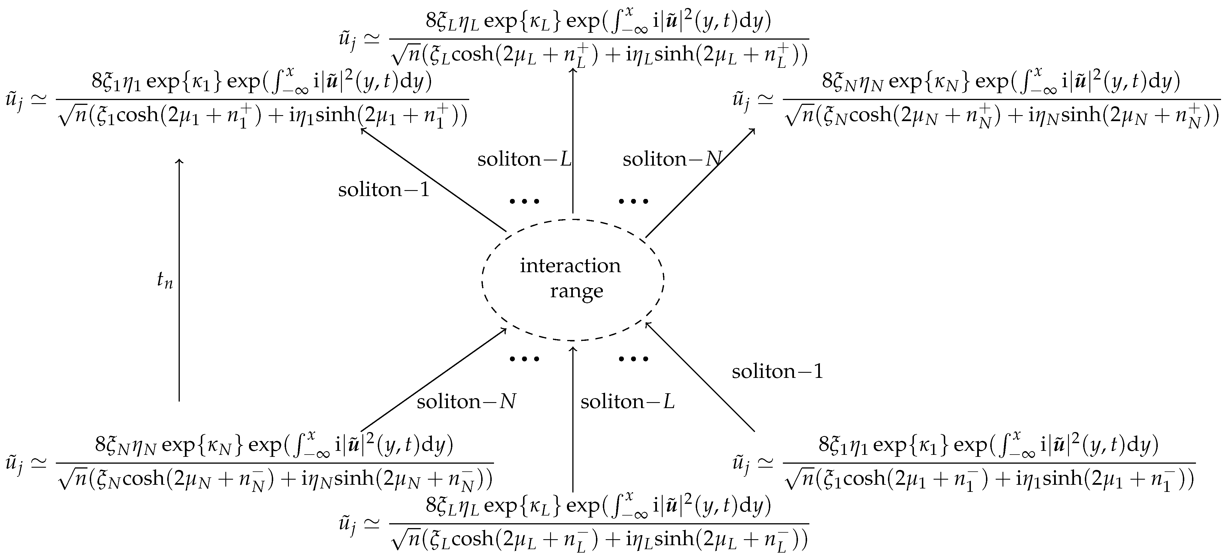
When $3{({\xi }_1^2-{\eta }_1^2)}^2-4{\xi }_1^2{\eta }_1^2\ne 3{({\xi }_2^2-{\eta }_2^2)}^2-4{\xi }_2^2{\eta }_2^2\ne \cdots \ne 3{({\xi }_N^2-{\eta }_N^2)}^2-4{\xi }_N^2{\eta }_N^2$, the asymptotic behavior of $q_j(x,t)$ is given on the limit $t_{\tilde{n}}\to \mp \infty$. Without loss of generality, assume $3{({\xi }_1^2-{\eta }_1^2)}^2-4{\xi }_1^2{\eta }_1^2>3{({\xi }_2^2-{\eta }_2^2)}^2-4{\xi }_2^2{\eta }_2^2>\cdots >3{({\xi }_N^2-{\eta }_N^2)}^2-4{\xi }_N^2{\eta }_N^2$.

In one case, according to the above assumption, it can be known that

$$\mathrm{Re}({\zeta }_1)\gg \mathrm{Re}({\zeta }_2)\gg \cdots \gg \mathrm{Re}({\zeta }_N),$$

(81)

when $t_{\tilde{n}}\to -\infty$. Then, we consider the N region $(1^{-})$–$(N^{-})$ with the following definitions, respectively:

$$(1^{-})\mathrm{Finite}\mathrm{Re}({\zeta }_1), (\mathrm{Re}({\zeta }_2),\mathrm{Re}({\zeta }_3),\cdots ,\mathrm{Re}({\zeta }_N))\to -\infty .$$

The dominant terms contain the factor ${\mathrm{e}}^{-({\zeta }_2+{\zeta }_2^{*}+\cdots +{\zeta }_N+{\zeta }_N^{*})}$. Then, the numerator of $u_j(x,t)$ with the factor ${\mathrm{e}}^{-({\zeta }_2+{\zeta }_2^{*}+\cdots +{\zeta }_N+{\zeta }_N^{*})}$ is

$$-4\mathrm{i}{c}_{1,j+1}^{*}{c}_{11}{\displaystyle \prod _{k=2}^N}|c_{k,1}{|}^2{\mathrm{e}}^{{\zeta }_1^{*}-{\zeta }_1}\left|\begin{array}{cccc}1& 1& \cdots & 1\\ \frac{1}{{\lambda }_2^2-{\lambda }_1^{*2}}& \frac{1}{{\lambda }_2^2-{\lambda }_2^{*2}}& \cdots & \frac{1}{{\lambda }_2^2-{\lambda }_N^{*2}}\\ ⋮& ⋮& ⋮& ⋮\\ \frac{1}{{\lambda }_N^2-{\lambda }_1^{*2}}& \frac{1}{{\lambda }_N^2-{\lambda }_2^{*2}}& \cdots & \frac{1}{{\lambda }_N^2-{\lambda }_N^{*2}}\end{array}\right|exp({\int }_{-\infty }^x\mathrm{i}|\tilde{\mathit{u}}{|}^2(y,t)\mathrm{d}y),$$

(82)

and the denominator of $u_j(x,t)$ is

$$\begin{array}{cc}& \frac{2}{{\lambda }_1^2-{\lambda }_1^{*2}}\left(\sum _{m=1}^n{|c_{1,m+1}|}^2{\mathrm{e}}^{{\zeta }_1+{\zeta }_1^{*}}\right){\displaystyle \prod _{k=2}^N}|c_{k,1}{|}^2\left|\begin{array}{cccc}\frac{1}{{\lambda }_2^2-{\lambda }_2^{*2}}& \frac{1}{{\lambda }_3^2-{\lambda }_2^{*2}}& \cdots & \frac{1}{{\lambda }_N^2-{\lambda }_2^{*2}}\\ ⋮& ⋮& ⋮& ⋮\\ \frac{1}{{\lambda }_2^2-{\lambda }_N^{*2}}& \frac{1}{{\lambda }_3^2-{\lambda }_N^{*2}}& \cdots & \frac{1}{{\lambda }_N^2-{\lambda }_N^{*2}}\end{array}\right|exp({\int }_{-\infty }^x\mathrm{i}|\tilde{\mathit{u}}{|}^2(y,t)\mathrm{d}y)\hfill \\ & +{\displaystyle \prod _{k=1}^N}|c_{k,1}{|}^2{\mathrm{e}}^{-{\zeta }_1-{\zeta }_1^{*}}\left|\begin{array}{cccc}\frac{1}{{\lambda }_1^2-{\lambda }_1^{*2}}& \frac{1}{{\lambda }_2^2-{\lambda }_1^{*2}}& \cdots & \frac{1}{{\lambda }_N^2-{\lambda }_1^{*2}}\\ \frac{1}{{\lambda }_1^2-{\lambda }_2^{*2}}& \frac{1}{{\lambda }_2^2-{\lambda }_2^{*2}}& \cdots & \frac{1}{{\lambda }_N^2-{\lambda }_2^{*2}}\\ ⋮& ⋮& ⋮& ⋮\\ \frac{1}{{\lambda }_1^2-{\lambda }_N^{*2}}& \frac{1}{{\lambda }_1^2-{\lambda }_N^{*2}}& \cdots & \frac{1}{{\lambda }_N^2-{\lambda }_N^{*2}}\end{array}\right|exp({\int }_{-\infty }^x\mathrm{i}|\tilde{\mathit{u}}{|}^2(y,t)\mathrm{d}y).\hfill \end{array}$$

(83)

Then, the asymptotic state of the solution (77) is

$$\begin{array}{cc}\hfill {\tilde{u}}_j(x,t_{\tilde{n}})\simeq & -2\mathrm{i}({\lambda }_1^2-{\lambda }_1^{*2})\frac{c_{1,1}{c}_{1,j+1}^{*}{c}_1^{-}{\mathrm{e}}^{{\zeta }_1^{*}-{\zeta }_1}exp({\int }_{-\infty }^x\mathrm{i}|\tilde{\mathit{u}}{|}^2(y,t)\mathrm{d}y)}{{\lambda }_1^{*}|c_{1,1}{|}^2{\mathrm{e}}^{-{\zeta }_1-{\zeta }_1^{*}}+{\lambda }_1{|c_1^{-}|}^2\left({\displaystyle \sum _{m=1}^n}{|c_{1,m+1}|}^2\right){\mathrm{e}}^{{\zeta }_1^{*}+{\zeta }_1}}\hfill \\ \hfill =& {\displaystyle \frac{8{\xi }_1{\eta }_{1}exp\{{\kappa }_1\}exp({\int }_{-\infty }^x\mathrm{i}|\tilde{\mathit{u}}{|}^2(y,t)\mathrm{d}y)}{\sqrt{n}({\xi }_1\cosh (2{\mu }_1+n_1^{-})+\mathrm{i}{\eta }_1\sinh (2{\mu }_1+n_1^{-}))}},\hfill \end{array}$$

(84)

where ${\kappa }_1=-2\mathrm{i}({\xi }_1^2-{\eta }_1^2)x+8\mathrm{i}{\displaystyle \sum _{0\le m_2\le \tilde{n}}}{(-1)}^{\frac{m_2+2}{2}}{C}_{\tilde{n}}^{m_2}{(2{\xi }_1{\eta }_1)}^{m_2}{({\xi }_1^2-{\eta }_1^2)}^{\tilde{n}-m_2}{t}_{\tilde{n}},c_{1,1}=c_{1,m+1}=1,{\mu }_1=-2{\xi }_1{\eta }_{1}x+8{\displaystyle \sum _{0\le m_1\le \tilde{n}}}{(-1)}^{\frac{m_1+1}{2}}{C}_{\tilde{n}}^{m_1}{(2{\xi }_1{\eta }_1)}^{m_1}{({\xi }_1^2-{\eta }_1^2)}^{\tilde{n}-m_1}{t}_{\tilde{n}},1\le m\le n,\sqrt{n}{c}_1^{-}={\mathrm{e}}^{n_1^{-}},c_1^{-}={\displaystyle \prod _{k\ne 1}^N}\frac{{\lambda }_1-{\lambda }_k^{*}}{{\lambda }_1-{\lambda }_k}$; $m_1$ is an odd number and $m_2$ is an even number.

$$(L^{-})(\mathrm{Re}({\zeta }_1),\cdots ,\mathrm{Re}({\zeta }_{L-1}))\to +\infty ,\mathrm{finite}\mathrm{Re}({\zeta }_L),(\mathrm{Re}({\zeta }_{L+1}),\cdots ,\mathrm{Re}({\zeta }_N))\to -\infty .$$

The dominant terms contain the factor ${\mathrm{e}}^{{\zeta }_1+{\zeta }_1^{*}+\cdots +{\zeta }_{L-1}+{\zeta }_{L-1}^{*}-({\zeta }_{L+1}+{\zeta }_{L+1}^{*}+\cdots +{\zeta }_N+{\zeta }_N^{*})}$. Then, the asymptotic state of the solution (77) is

$$\begin{array}{cc}\hfill {\tilde{u}}_j(x,t)\simeq & -2\mathrm{i}({\lambda }_L^2-{\lambda }_L^{*2}){\displaystyle \frac{{\displaystyle \prod _{k_1\ne L}^N}(c_{L,2}{c}_{L,j+1}^{*}{\displaystyle \prod _{k_1\ne L}^N}{\displaystyle \sum _{m=1}^n}|c_{k_1,m+1}{|}^2-c_{L,1}{\displaystyle \frac{{\lambda }_k^2-{\lambda }_k^{*2}}{{\lambda }_k^2-{\lambda }_L^{*2}}}{\displaystyle \prod _{k_1\ne L}^N}{c}_{k_1,j+1}^{*}{\displaystyle \sum _{m=1}^n}{c}_{L,m+1}^{*}{c}_{k_1,m+1}){\mathrm{e}}^{{\zeta }_L^{*}-{\zeta }_L}exp({\int }_{-\infty }^x\mathrm{i}|\tilde{\mathit{u}}{|}^2(y,t)\mathrm{d}y)}{{\lambda }_L^{*}|c_L^{-}{|}^2{\displaystyle \prod _{k_1\ne L}^N}{\displaystyle \sum _{m=1}^n}|c_{k_1,m+1}{|}^2|c_{L,1}{|}^2{\mathrm{e}}^{-({\zeta }_L^{*}+{\zeta }_L)}+{\lambda }_L{\displaystyle \prod _{k_1\ne L}^N}({\displaystyle \sum _{m_1=1}^n}{\displaystyle \sum _{m_2=1}^n}|c_{k_1,m_1+1}{|}^2|c_{L,m_2+1}{|}^2){\mathrm{e}}^{{\zeta }_L^{*}+{\zeta }_L}}}\hfill \\ \hfill =& {\displaystyle \frac{8{\xi }_L{\eta }_{L}exp\{{\kappa }_L\}exp({\int }_{-\infty }^x\mathrm{i}|\tilde{\mathit{u}}{|}^2(y,t)\mathrm{d}y)}{\sqrt{n}({\xi }_L\cosh (2{\mu }_L+n_L^{-})+\mathrm{i}{\eta }_L\sinh (2{\mu }_L+n_L^{-}))}},\hfill \end{array}$$

(85)

where ${\kappa }_L=-2\mathrm{i}({\xi }_L^2-{\eta }_L^2)x+8\mathrm{i}{\displaystyle \sum _{0\le m_2\le \tilde{n}}}{(-1)}^{\frac{m_2+2}{2}}{C}_{\tilde{n}}^{m_2}{(2{\xi }_L{\eta }_L)}^{m_2}{({\xi }_L^2-{\eta }_L^2)}^{\tilde{n}-m_2}{t}_{\tilde{n}},c_{k_1,m+1}=c_{L,m+1}=c_{L,1}=1,{\mu }_L=-2{\xi }_L{\eta }_{L}x+8{\displaystyle \sum _{0\le m_1\le \tilde{n}}}{(-1)}^{\frac{m_1+1}{2}}{C}_{\tilde{n}}^{m_1}{(2{\xi }_L{\eta }_L)}^{m_1}{({\xi }_L^2-{\eta }_L^2)}^{\tilde{n}-m_1}{t}_{\tilde{n}},$$1\le m\le n,{\displaystyle \frac{\sqrt{n}}{c_L^{-}}}=e^{n_L^{-}},c_L^{-}={\displaystyle \prod _{k\ne L}^N}{\displaystyle \frac{{\lambda }_k^2-{\lambda }_L^{*2}}{{\lambda }_k^{*2}-{\lambda }_L^{*2}}}$.

$$(N^{-})(\mathrm{Re}({\zeta }_1),\cdots ,\mathrm{Re}({\zeta }_{N-1}))\to +\infty ,\mathrm{finite}\mathrm{Re}({\zeta }_N).$$

The dominant terms contain the factor ${\mathrm{e}}^{{\zeta }_1+{\zeta }_1^{*}+\cdots +{\zeta }_{N-1}+{\zeta }_{N-1}^{*}}$. With calculations similar to those in the case of $(L^{-})$, we obtain the asymptotic state of ${\tilde{u}}_j(x,t)$ given by Equation (85) with $L=N$.

In another case, it is easy to know that

$$\mathrm{Re}({\zeta }_1)\ll \mathrm{Re}({\zeta }_2)\ll \cdots \ll \mathrm{Re}({\zeta }_{\mathrm{N}}),$$

(86)

when $t_{\tilde{n}}\to +\infty$. Similarly, we consider the N region $(1^{+})$–$(N^{+})$, respectively.

$$(1^{+})\mathrm{Finite}\mathrm{Re}({\zeta }_1),(\mathrm{Re}({\zeta }_2),\cdots ,\mathrm{Re}({\zeta }_N))\to +\infty .$$

The dominant terms contain the factor ${\mathrm{e}}^{{\zeta }_2+{\zeta }_2^{*}+\cdots +{\zeta }_N+{\zeta }_N^{*}}$, and the asymptotic state is

$$\begin{array}{cc}\hfill {\tilde{u}}_j(x,t)\simeq & -2\mathrm{i}({\lambda }_1^2-{\lambda }_1^{*2}){\displaystyle \frac{{\displaystyle \prod _{k_1\ne 1}^N}{c}_{1,1}(c_{1,j+1}^{*}{\displaystyle \prod _{k_1\ne 1}^N}{\displaystyle \sum _{m=1}^n}|c_{k_1,m+1}{|}^2-{\displaystyle \frac{{\lambda }_k^2-{\lambda }_k^{*2}}{{\lambda }_k^2-{\lambda }_1^{*2}}}{\displaystyle \prod _{k_1\ne 1}^N}{c}_{k_1,j+1}^{*}{\displaystyle \sum _{m=1}^n}{c}_{1,m+1}^{*}{c}_{k_1,m+1}){\mathrm{e}}^{{\zeta }_1^{*}-{\zeta }_1}exp({\int }_{-\infty }^x\mathrm{i}|\tilde{\mathit{u}}{|}^2(y,t)\mathrm{d}y)}{{\lambda }_1^{*}{\displaystyle \prod _{k_1\ne 1}^N}{\displaystyle \sum _{m=1}^n}|c_{k_1,m+1}{|}^2|c_{1,1}{|}^2{\mathrm{e}}^{-({\zeta }_1^{*}+{\zeta }_1)}+{\lambda }_1|c_1^{+}{|}^2{\displaystyle \prod _{k_1\ne 1}^N}({\displaystyle \sum _{m_1=1}^n}{\displaystyle \sum _{m_2=1}^n}|c_{1,m_1+1}{|}^2|c_{k_1,m_2+1}{|}^2)e^{{\zeta }_1^{*}+{\zeta }_1}}}\hfill \\ \hfill =& {\displaystyle \frac{8{\xi }_1{\eta }_{1}exp\{{\kappa }_1\}exp({\int }_{-\infty }^x\mathrm{i}|\tilde{\mathit{u}}{|}^2(y,t)\mathrm{d}y)}{\sqrt{n}({\xi }_1\cosh (2{\mu }_1+n_1^{+})+\mathrm{i}{\eta }_1\sinh (2{\mu }_1+n_1^{+}))}},\hfill \end{array}$$

(87)

where $c_{1,1}=c_{1,m+1}=c_{k_1,m+1}=1,1\le m\le n,\sqrt{n}{c}_1^{+}={\mathrm{e}}^{n_1^{+}},c_1^{+}={\displaystyle \prod _{k\ne 1}^N}{\displaystyle \frac{{\lambda }_k^{*2}-{\lambda }_1^{*2}}{{\lambda }_k^2-{\lambda }_1^{*2}}}$.

$$(L^{+})(\mathrm{Re}({\zeta }_1),\cdots ,\mathrm{Re}({\zeta }_{L-1}))\to -\infty ,\mathrm{finite}\mathrm{Re}({\zeta }_L),(\mathrm{Re}({\zeta }_{L+1}),\cdots ,\mathrm{Re}({\zeta }_N))\to +\infty .$$

The dominant terms contain the factor ${\mathrm{e}}^{-({\zeta }_1+{\zeta }_1^{*}+\cdots +{\zeta }_{L-1}+{\zeta }_{L-1}^{*})+{\zeta }_{L+1}+{\zeta }_{L+1}^{*}+\cdots +{\zeta }_N+{\zeta }_N^{*}}$, and the asymptotic state is

$$\begin{array}{cc}\hfill {\tilde{u}}_j(x,t)\simeq & -2\mathrm{i}({\lambda }_L^2-{\lambda }_L^{*2}){\displaystyle \frac{c_L^{+}{c}_{L,1}{c}_{L,j+1}^{*}{\mathrm{e}}^{{\zeta }_L^{*}-{\zeta }_L}exp({\int }_{-\infty }^x\mathrm{i}|\tilde{\mathit{u}}{|}^2(y,t)\mathrm{d}y)}{{\displaystyle \sum _{m=1}^n}|c_{L,m+1}{|}^2{\mathrm{e}}^{{\zeta }_L^{*}+{\zeta }_L}+|c_L^{+}{|}^2{|c_{L,1}|}^2{\mathrm{e}}^{-({\zeta }_L^{*}+{\zeta }_L)}}}\hfill \\ \hfill =& {\displaystyle \frac{8{\xi }_L{\eta }_{L}exp\{{\kappa }_L\}exp({\int }_{-\infty }^x\mathrm{i}|\tilde{\mathit{u}}{|}^2(y,t)\mathrm{d}y)}{\sqrt{n}({\xi }_L\cosh (2{\mu }_L+n_L^{+})+\mathrm{i}{\eta }_L\sinh (2{\mu }_L+n_L^{+}))}},\hfill \end{array}$$

(88)

where $c_{L,1}=c_{L,m+1}=1,1\le m\le n,{\displaystyle \frac{\sqrt{n}}{c_L^{+}}}=e^{n_L^{+}},c_L^{+}={\displaystyle \prod _{k\ne L}^N}{\displaystyle \frac{{\lambda }_L^2-{\lambda }_k^2}{{\lambda }_L^2-{\lambda }_k^{*2}}}$.

$$(N^{+})(\mathrm{Re}({\zeta }_1),\cdots ,\mathrm{Re}({\zeta }_{N-1}))\to -\infty ,\mathrm{finite}\mathrm{Re}({\zeta }_N).$$

The dominant terms contain the factor ${\mathrm{e}}^{-({\zeta }_1+{\zeta }_1^{*}+\cdots +{\zeta }_{N-1}+{\zeta }_{N-1}^{*})}$. With calculations similar to those in the case $(L^{+})$, we obtain the asymptotic form of ${\tilde{u}}_j(x,t)$ given by Equation (88) with $L=N$.

If we combine Equations (84) and (85), or Equations (87) and (88), it is easy to obtain the following theorem.

Theorem 1.

The long-time asymptotic states of the N-soliton solution of the n-th mHOCLL system are as follows (see Figure 2):

when $t_{\tilde{n}}\to -\infty ,$

$$\begin{array}{cc}\hfill {\tilde{u}}_j(x,t_{\tilde{n}})& \simeq {\displaystyle \frac{8{\xi }_l{\eta }_{l}exp\{{\kappa }_l\}exp({\int }_{-\infty }^x\mathrm{i}|\tilde{\mathbf{u}}{|}^2(y,t)\mathrm{d}y)}{\sqrt{n}({\xi }_l\cosh (2{\mu }_l+n_l^{-})+\mathrm{i}{\eta }_l\sinh (2{\mu }_l+n_l^{-}))}},\hfill \end{array}$$

(89)

when $t_{\tilde{n}}\to +\infty ,$

$$\begin{array}{cc}\hfill {\tilde{u}}_j(x,t_{\tilde{n}})& \simeq {\displaystyle \frac{8{\xi }_l{\eta }_{l}exp\{{\kappa }_l\}exp({\int }_{-\infty }^x\mathrm{i}|\tilde{\mathbf{u}}{|}^2(y,t)\mathrm{d}y)}{\sqrt{n}({\xi }_l\cosh (2{\mu }_l+n_l^{+})+\mathrm{i}{\eta }_l\sinh (2{\mu }_l+n_l^{+}))}},\hfill \end{array}$$

(90)

where

$$\begin{array}{cc}\hfill & {\mu }_l=-2{\xi }_l{\eta }_{l}x+8{\displaystyle \sum _{0\le m_1\le \tilde{n}}}{C}_n^{m_1}{(-1)}^{\frac{m_1+1}{2}}{(2{\xi }_l{\eta }_l)}^{m_1}{({\xi }_l^2-{\eta }_l^2)}^{\tilde{n}-m_1}{t}_{\tilde{n}},\hfill \\ \hfill & {\kappa }_l=-2\mathrm{i}({\xi }_l^2-{\eta }_l^2)x+8\mathrm{i}{\displaystyle \sum _{0\le m_2\le \tilde{n}}}{C}_n^{m_2}{(-1)}^{\frac{m_2+2}{2}}{(2{\xi }_l{\eta }_l)}^{m_2}{({\xi }_l^2-{\eta }_l^2)}^{\tilde{n}-m_2}{t}_{\tilde{n}},\hfill \end{array}$$

with $c_{k,m+1}=1,0\le m\le n,1\le k\le N,\sqrt{n}{c}_1^{-}={\mathrm{e}}^{n_1^{-}},c_1^{-}={\displaystyle \prod _{k\ne 1}^N}\frac{{\lambda }_1^2-{\lambda }_k^{*2}}{{\lambda }_1^2-{\lambda }_k^2},{\displaystyle \frac{\sqrt{n}}{c_L^{-}}}={\mathrm{e}}^{n_L^{-}},c_L^{-}={\displaystyle \prod _{k\ne L}^N}\frac{{\lambda }_k^2-{\lambda }_L^{*2}}{{\lambda }_k^{*2}-{\lambda }_L^{*2}},\sqrt{n}{c}_1^{+}={\mathrm{e}}^{n_1^{+}},c_1^{+}={\displaystyle \prod _{k\ne 1}^N}\frac{{\lambda }_k^{*2}-{\lambda }_1^{*2}}{{\lambda }_k^2-{\lambda }_1^{*2}},{\displaystyle \frac{\sqrt{n}}{c_L^{+}}}={\mathrm{e}}^{n_L^{+}},c_L^{+}={\displaystyle \prod _{k\ne L}^N}\frac{{\lambda }_L^2-{\lambda }_k^2}{{\lambda }_L^2-{\lambda }_k^{*2}}$; $m_1$ is an odd number and $m_2$ is an even number.

Theorem 1 defines the collision laws of N-solitons in the n-th mHOCLL system.

4.2. One-Soliton Solutions

When $N=1$, the solution (77) is

$${\tilde{u}}_j=-2\mathrm{i}({\lambda }_1^2-{\lambda }_1^{*2}){\displaystyle \frac{c_{11}{c}_{1,j+1}^{*}{\mathrm{e}}^{{\zeta }_1^{*}-{\zeta }_1}exp({\int }_{-\infty }^x\mathrm{i}|\tilde{\mathit{u}}{|}^2(y,t)\mathrm{d}y)}{{\lambda }_1^{*}|c_{11}{|}^2{\mathrm{e}}^{-({\zeta }_1^{*}+{\zeta }_1)}+{\lambda }_1{\displaystyle \sum _{m=1}^n}{|c_{1,m+1}|}^2{\mathrm{e}}^{{\zeta }_1^{*}+{\zeta }_1}}},1\le j\le n.$$

(91)

Letting

$${\lambda }_1=\xi +\mathrm{i}\eta ,c_{1,1}=\sqrt{n}{\mathrm{e}}^{-2\eta x_0+\mathrm{i}{\sigma }_0},c_{1,m+1}=1,1\le m\le n,$$

(92)

we can rewrite Equation (91) as

$$\begin{array}{c}\hfill {\tilde{u}}_j={\displaystyle \frac{8\xi \eta exp\{-2\mathrm{i}({\xi }^2-{\eta }^2)x+8\mathrm{i}{\displaystyle \sum _{0\le m_2\le \tilde{n}}}{(-1)}^{\frac{m_2+2}{2}}{C}_{\tilde{n}}^{m_2}{(2\xi \eta )}^{m_2}{({\xi }^2-{\eta }^2)}^{\tilde{n}-m_2}{t}_{\tilde{n}}+\mathrm{i}{\sigma }_0\}exp({\int }_{-\infty }^x\mathrm{i}|\tilde{\mathit{u}}{|}^2(y,t)\mathrm{d}y)}{\sqrt{n}(\xi \cosh \tau +\mathrm{i}\eta \sinh \tau )}},\end{array}$$

(93)

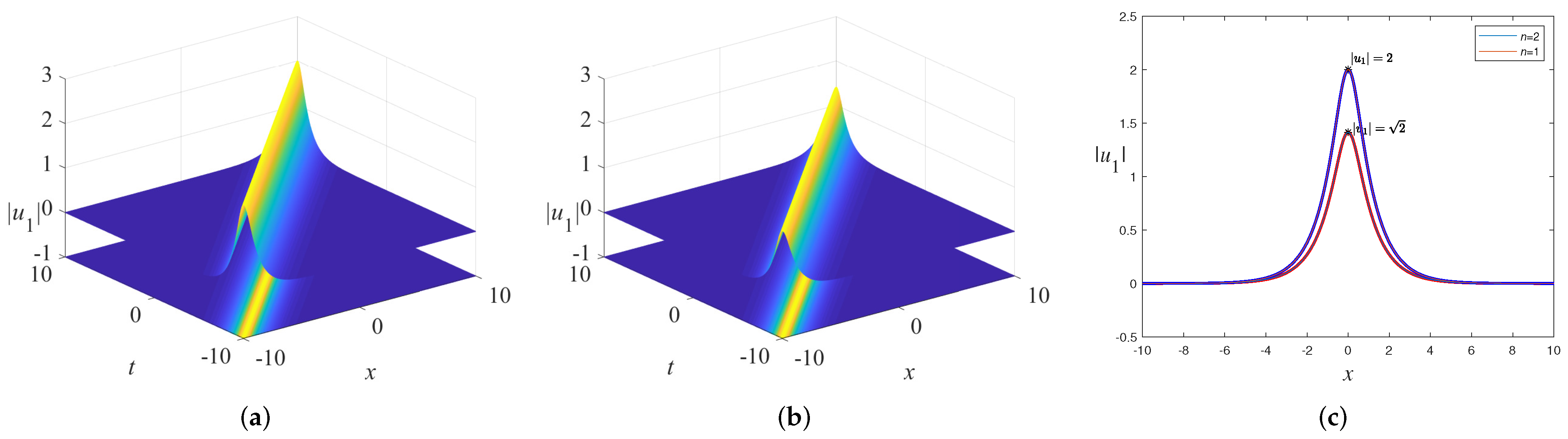
where ${\xi }_0,x_0$ and ${\sigma }_0$ are real parameters, $\tau =-4\xi \eta x+8{\displaystyle \sum _{0\le m_1\le \tilde{n}}}{(-1)}^{\frac{m_1+1}{2}}{C}_{\tilde{n}}^{m_1}{(2\xi \eta )}^{m_1}{({\xi }^2-{\eta }^2)}^{\tilde{n}-m_1}{t}_{\tilde{n}}+\eta x_0$, $m_1$ is odd number, and $m_2$ is even number. Without loss of generality, we give two cases of a one-soliton solution in Figure 3.

From Figure 3, we can see that the amplitude of the solitary wave decreases as n increases. Its peak amplitude and velocity are ${\displaystyle \frac{8}{\sqrt{n}}}\xi \eta$, and $-8{\displaystyle \sum _{0\le m_1\le \tilde{n}}}{(-1)}^{\frac{m_1+1}{2}}{C}_{\tilde{n}}^{m_1}{(2\xi \eta )}^{m_1-1}$${({\xi }^2-{\eta }^2)}^{\tilde{n}-m_1}$, respectively. The phase of the solution is linearly related to space x and time $t_{\tilde{n}}$. The spatial gradient of the phase is proportional to the wave velocity.

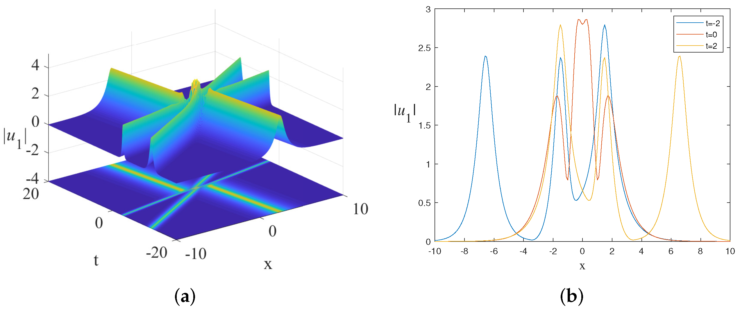
4.3. Two-Soliton Solution

When $N=2$, the solution (77) is

$${\tilde{u}}_j=4\mathrm{i}{\displaystyle \frac{det\widehat{{\rm Y}}}{det{\rm Y}}}exp({\int }_{-\infty }^x\mathrm{i}|\tilde{\mathit{u}}{|}^2(y,t)\mathrm{d}y),1\le j\le n,$$

(94)

where

$$\widehat{{\rm Y}}=\left(\begin{array}{ccc}0& c_{11}{\mathrm{e}}^{-{\zeta }_1}& c_{21}{\mathrm{e}}^{-{\zeta }_2}\\ c_{1,j+1}^{*}{\mathrm{e}}^{{\zeta }_1^{*}}& {\upsilon }_{11}& {\upsilon }_{12}\\ c_{2,j+1}^{*}{\mathrm{e}}^{{\zeta }_2^{*}}& {\upsilon }_{21}& {\upsilon }_{22}\end{array}\right),$$

(95)

and

$${\rm Y}=\left(\begin{array}{cc}{\upsilon }_{11}& {\upsilon }_{12}\\ {\upsilon }_{21}& {\upsilon }_{22}\end{array}\right),$$

(96)

with

$${\upsilon }_{kl}={\displaystyle \frac{2}{{\lambda }_l^2-{\widehat{\lambda }}_k^2}}({\lambda }_l{\displaystyle \sum _{m=1}^n}(c_{k,m+1}^{*}{c}_{l,m+1}){\mathrm{e}}^{{\zeta }_k^{*}+{\zeta }_l}+{\widehat{\lambda }}_k{c}_{k,1}^{*}{c}_{l,1}{\mathrm{e}}^{-({\zeta }_k^{*}+{\zeta }_l)}),k,l=1,2.$$

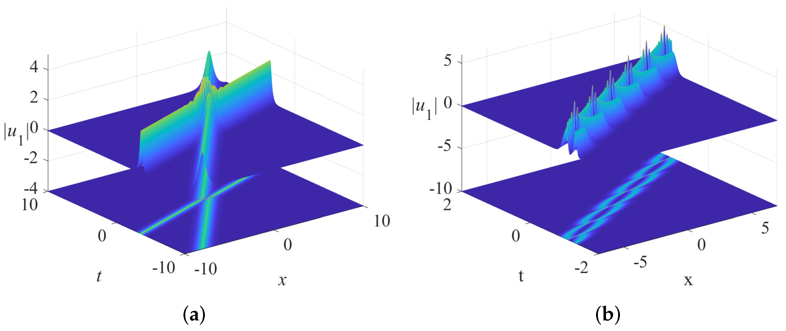
According to the factor of the exponential function in Equations (77)–(79), we can know that there are two different states of the two-soliton solution. One is $3{({\xi }_1^2-{\eta }_1^2)}^2-4{\xi }_1^2{\eta }_1^2\ne 3{({\xi }_2^2-{\eta }_2^2)}^2-4{\xi }_2^2{\eta }_2^2$, the other one is $3{({\xi }_1^2-{\eta }_1^2)}^2-4{\xi }_1^2{\eta }_1^2=3{({\xi }_2^2-{\eta }_2^2)}^2-4{\xi }_2^2{\eta }_2^2$. Without loss of generality, we take

$${\lambda }_1=1-0.6\mathrm{i},{\lambda }_2=-0.6+0.7\mathrm{i},c_{1,1}=c_{2,1}=c_{1,2}=c_{2,2}=1,$$

(97)

which makes the two-soliton solution elastically collide as shown in Figure 4a. Similarly, when we take

$${\lambda }_1=1+\sqrt{\frac{5}{3}-\frac{\sqrt{46}}{6}}\mathrm{i},{\lambda }_2=1.1+\sqrt{\frac{121}{60}-\frac{\sqrt{47314}}{150}}\mathrm{i},c_{1,1}=c_{2,1}=c_{1,2}=c_{2,2}=1,$$

(98)

the two-soliton solution appears in the bound state shown in Figure 4b. Note that we only provide the figures for $|u_1|$ with $n=1$.

From Figure 4a, it can be seen that when $\mathrm{Re}({\lambda }_1^4)+2{\mathrm{Re}}^2({\lambda }_1^2)\ne \mathrm{Re}({\lambda }_2^4)+2{\mathrm{Re}}^2({\lambda }_2^2)$, the solution contains two single-solitons which are far apart and moving toward each other as $t_{\tilde{n}}\to \infty$. When they collide, they interact strongly. However, when $t_{\tilde{n}}\to \infty$, they reappear from the interaction without changing shape or velocity; that is, no energy radiation is emitted into the far field. Hence, the interactions of the solitons are elastic. The elastic collision is one of the most important characteristics of solitary waves, which can indicate that the mHOCLL system (22) is integrable. However, although the elastic collision occurs, it will inevitably leave some collision marks. From Figure 4, we can see that after the collision, each soliton is position-shifted and phase-shifted.

4.4. Three-Soliton Solution

When $N=3$, the solution (77) is

$${\tilde{u}}_j=4\mathrm{i}{\displaystyle \frac{det\widehat{{\rm Y}}}{det{\rm Y}}}exp({\int }_{-\infty }^x\mathrm{i}|\tilde{\mathit{u}}{|}^2(y,t)\mathrm{d}y),1\le j\le n,$$

(99)

where

$$\widehat{{\rm Y}}=\left(\begin{array}{cccc}0& c_{11}{\mathrm{e}}^{-{\zeta }_1}& c_{21}{\mathrm{e}}^{-{\zeta }_2}& c_{31}{\mathrm{e}}^{-{\zeta }_3}\\ c_{1,j+1}^{*}{\mathrm{e}}^{{\zeta }_1^{*}}& {\upsilon }_{11}& {\upsilon }_{12}& {\upsilon }_{13}\\ c_{2,j+1}^{*}{\mathrm{e}}^{{\zeta }_2^{*}}& {\upsilon }_{21}& {\upsilon }_{22}& {\upsilon }_{23}\\ c_{3,j+1}^{*}{\mathrm{e}}^{{\zeta }_3^{*}}& {\upsilon }_{31}& {\upsilon }_{32}& {\upsilon }_{33}\end{array}\right),$$

(100)

and

$${\rm Y}=\left(\begin{array}{ccc}{\upsilon }_{11}& {\upsilon }_{12}& {\upsilon }_{13}\\ {\upsilon }_{21}& {\upsilon }_{22}& {\upsilon }_{23}\\ {\upsilon }_{31}& {\upsilon }_{32}& {\upsilon }_{33}\end{array}\right),$$

(101)

with

$${\upsilon }_{kl}={\displaystyle \frac{2}{{\lambda }_l^2-{\widehat{\lambda }}_k^2}}({\lambda }_l{\displaystyle \sum _{m=1}^n}(c_{k,m+1}^{*}{c}_{l,m+1}){\mathrm{e}}^{{\zeta }_k^{*}+{\zeta }_l}+{\widehat{\lambda }}_k{c}_{k,1}^{*}{c}_{l,1}{\mathrm{e}}^{-({\zeta }_k^{*}+{\zeta }_l)}),k,l=1,2,3.$$

Take

$${\lambda }_1=1-0.6\mathrm{i}, {\lambda }_2=-0.7+0.6\mathrm{i}, {\lambda }_3=0.4+0.7\mathrm{i}, c_{k,l}=1,( k,l=1,2,3);$$

(102)

we give the figures of three-soliton solution in Figure 5.

5. Conclusions

In this paper, an arbitrary order matrix spectral problem was used to generate the mHOCLL system. Meanwhile, the bi-Hamiltonian structure of this system was given by the trace identity. Then, the corresponding RH problem was constructed with zero background. To obtain the exact solution of the system, we discussed two cases of the RH problem. One was that the RH problem is regular. The other one was that the RH problem is non-regular and the scattering problem is reflectionless. When the jump matrix J was an identity matrix, the N-soliton solution of the mHOCLL system presented the explicit formulas, and its long-time asymptotic behavior was analyzed. Finally, we provided the determinant form of the N-soliton solution and the figures of one-, two-, three-soliton solutions as specific examples.

The RH method is a very efficient method for obtaining soliton solutions. We obtained some results in this paper and we look forward to studying multicomponent systems, which include different Lie algebras [38], quadratic spectral parameters [21,39,40], and polynomial spectral parameters [41]. In addition, we will investigate where the jump matrix can be obtained at non-zero boundary branch cuts and use the RH method to obtain rogue waves. Our results from the perspective of the RH method will hopefully be of great help in studying the exact solutions of integrable equations.