

An Extension on the Local Convergence for the Multi-Step Seventh Order Method with ψ-Continuity Condition in the Banach Spaces

 ,
,
Abstract
:1. Introduction
2. Local Convergence Analysis
3. Numerical Example
4. Conclusions
Author Contributions
Funding
Institutional Review Board Statement
Informed Consent Statement
Data Availability Statement
Conflicts of Interest
References
- Behl, R.; Motsa, S.S. Geometric construction of eighth-order optimal families of Ostrowski’s method. Sci. World J. 2015, 2015, 614612. [Google Scholar] [CrossRef] [PubMed]
- Sharma, J.R.; Arora, H. A new family of optimal eighth order methods with dynamics for nonlinear equations. Appl. Math. Comput. 2016, 273, 924–933. [Google Scholar] [CrossRef]
- Rall, L.B. Computational Solution of Nonlinear Operator Equations; Robert, E., Ed.; Krieger Publishing Company: New York, NY, USA, 1979. [Google Scholar]
- Regmi, S.; Argyros, C.I.; Argyros, I.K.; George, S. Extended convergence of a sixth order scheme for solving equations under–continuity conditions. Moroc. J. Pure Appl. Anal. 2022, 8, 92–101. [Google Scholar] [CrossRef]
- Sharma, J.R.; Argyros, I.K. Local convergence of a Newton-Traub composition in Banach spaces. SeMA 2018, 75, 57–68. [Google Scholar] [CrossRef]
- Traub, J.F. Iterative Methods for the Solution of Equations; Chelsea Publishing Company: New York, NY, USA, 1977. [Google Scholar]
- Kantorovich, L.V.; Akilov, G.P. Functional Analysis; Pergamon Press: Oxford, UK, 1982. [Google Scholar]
- Argyros, I.K.; George, S. Local convergence of two competing third order methods in Banach spaces. Appl. Math. 2016, 41, 341–350. [Google Scholar] [CrossRef]
- Argyros, I.K.; Khattri, S.K. Local convergence for a family of third order methods in Banach spaces, Punjab Univ. J. Math. 2016, 46, 52–63. [Google Scholar]
- Argyros, I.K.; Gonzalez, D.; Khattri, S.K. Local convergence of a one parameter fourth-order Jarratt-type method in Banach spaces. Comment. Math. Univ. Carol. 2016, 57, 289–300. [Google Scholar]
- Cordero, A.; Ezquerro, J.A.; Hernéz, M.A.; Torregrosa, J. On the local convergence of a fifth-order iterative method in Banach spaces. Appl. Math. Comput 2015, 251, 396–403. [Google Scholar] [CrossRef] [Green Version]
- Martínez, E.; Singh, S.; Hueso, J.L.; Gupta, D.K. Enlarging the convergence domain in local convergence studies for iterative methods in Banach spaces. Appl. Math. Comput. 2016, 281, 252–265. [Google Scholar] [CrossRef] [Green Version]
- Sharma, J.R.; Gupta, P. An efficient fifth order method for solving systems of nonlinear equations. Comput. Math. Appl. 2014, 67, 591–601. [Google Scholar] [CrossRef]
- Panday, B.; Jaiswal, J.P. On the local convergence of modified Homeier-like method in Banach spaces. Numer. Anal. Appl. 2018, 11, 332–345. [Google Scholar] [CrossRef]
- Xiao, X.; Yin, H. A new class of methods with higher order of convergence for solving systems of nonlinear equations. Appl. Math. Comput. 2015, 264, 300–309. [Google Scholar] [CrossRef]
- Saxena, A.; Jaiswal, J.P.; Pardasani, K.R. Broadening the convergence domain of Seventh-order method satisfying Lipschitz and Holder conditions. Results Nonlinear Anal. 2022, 5, 473–486. [Google Scholar] [CrossRef]
- Argyros, I.K.; Hilout, S. Computational Methods in Nonlinear Analysis; World Scientific Publishing Company: Singapore, 2013. [Google Scholar]
- Behl, R.; Argyros, I.K.; Mallawi, F.O. Some High-Order Convergent Iterative Procedures for Nonlinear Systems with Local Convergence. Mathematics 2021, 9, 1375. [Google Scholar] [CrossRef]
- Polyanin, A.D.; Manzhirov, A.V. Handbook of Integral Equations; Chapman and Hall/CRC: Florida, NY, USA, 1998. [Google Scholar]
- Argyros, I.K.; George, S. Increasing the order of convergence for iterative methods in Banach space under weak conditions. Malaya J. Mat. 2018, 6, 396–401. [Google Scholar] [CrossRef] [PubMed]


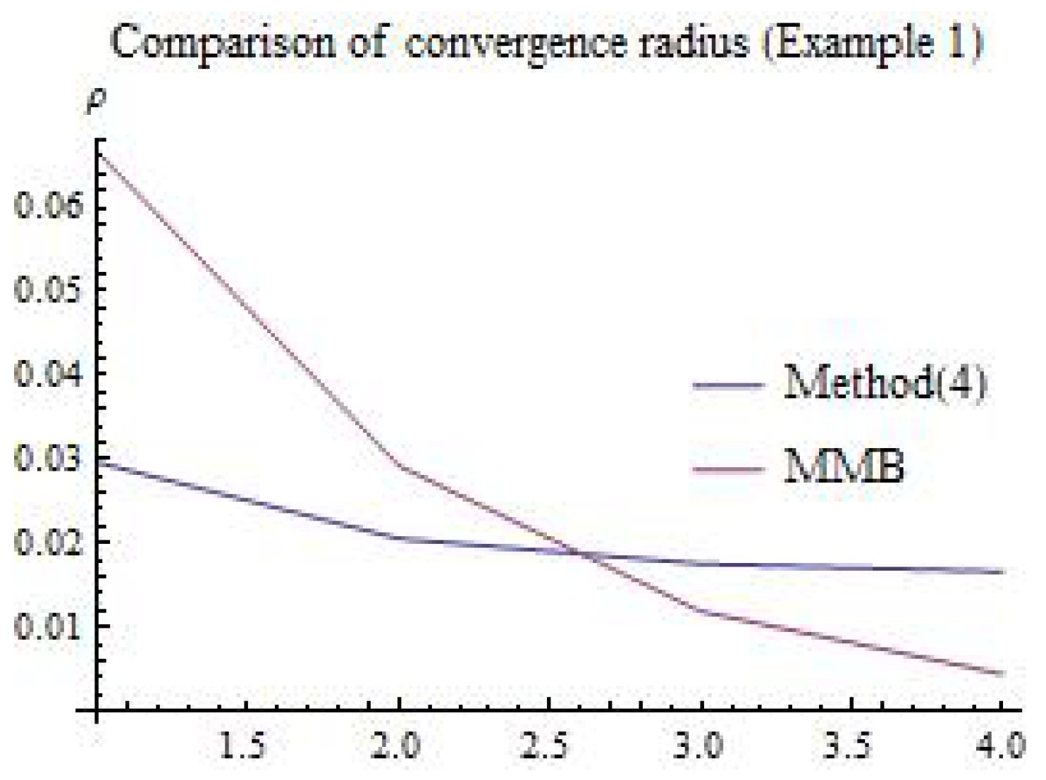
| Radius | |||||
|---|---|---|---|---|---|
| Method (4) | 0.0296296 | 0.0205601 | 0.0175449 | 0.0166341 | 0.0166341 |
| MMB | 0.0666667 | 0.0292298 | 0.0118907 | 0.00440901 | 0.00440901 |
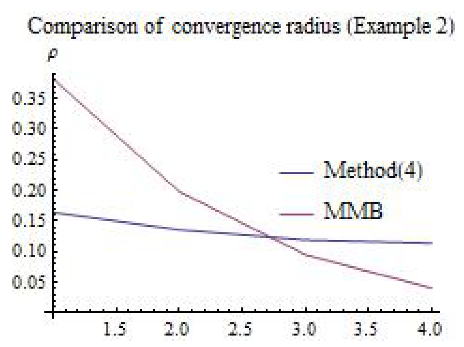
| Radius | |||||
|---|---|---|---|---|---|
| Method (4) | 0.164331 | 0.135757 | 0.119283 | 0.114151 | 0.114151 |
| MMB | 0.382692 | 0.198328 | 0.0949498 | 0.040525 | 0.040525 |
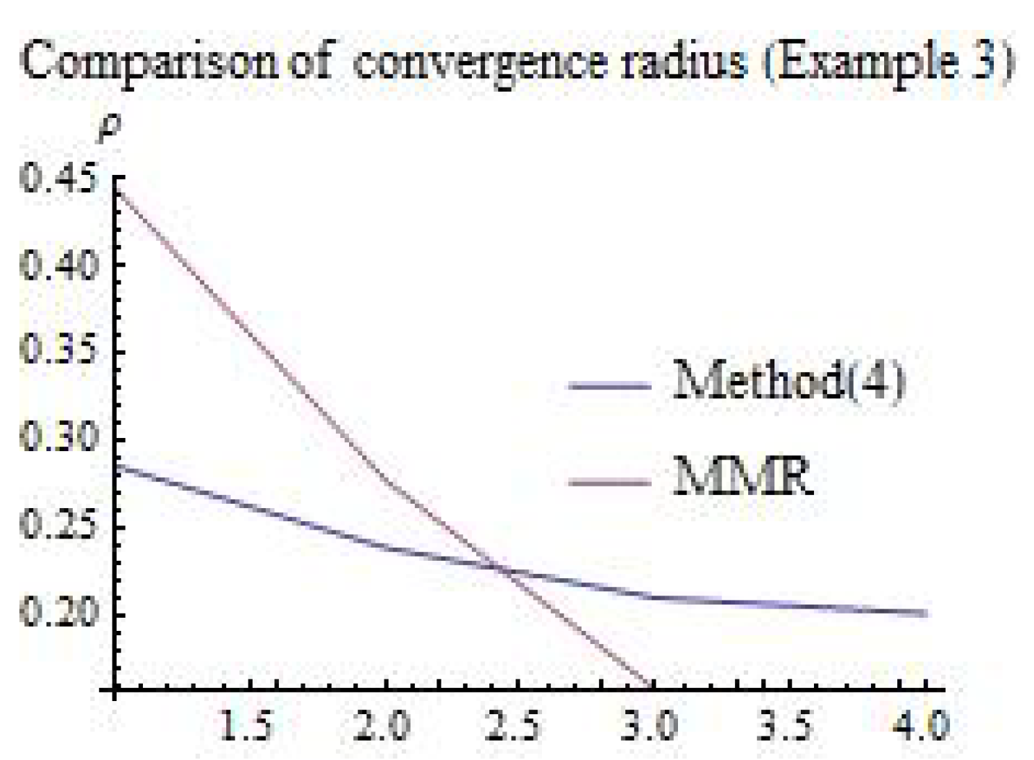
| Radius | |||||
|---|---|---|---|---|---|
| Method (4) | 0.285714 | 0.238655 | 0.210099 | 0.201186 | 0.201186 |
| MMR | 0.44444 | 0.277466 | 0.15771 | - | 0.15771 |
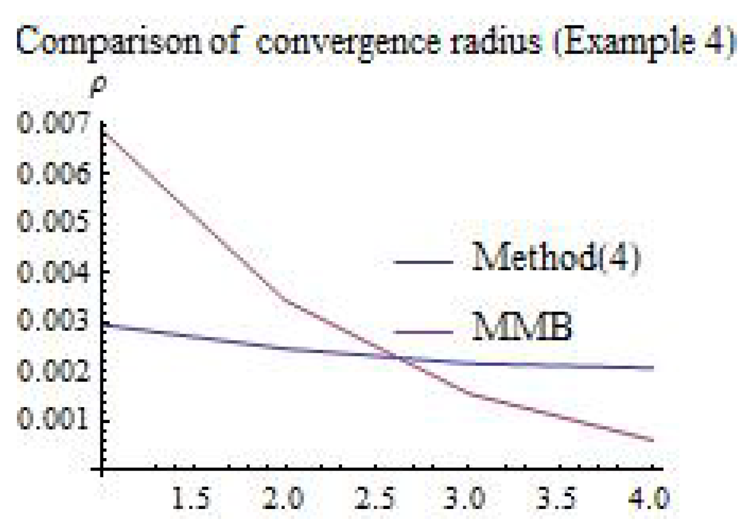
| Radius | |||||
|---|---|---|---|---|---|
| Method (4) | 0.00295578 | 0.00246894 | 0.00217353 | 0.00208131 | 0.00208131 |
| MMB | 0.00689682 | 0.00344841 | 0.0015606 | 0.000621105 | 0.000621105 |
Publisher’s Note: MDPI stays neutral with regard to jurisdictional claims in published maps and institutional affiliations. |
© 2022 by the authors. Licensee MDPI, Basel, Switzerland. This article is an open access article distributed under the terms and conditions of the Creative Commons Attribution (CC BY) license (https://creativecommons.org/licenses/by/4.0/).
Share and Cite
Darvishi, M.T.; Al-Obaidi, R.H.; Saxena, A.; Prakash Jaiswal, J.; Raj Pardasani, K. An Extension on the Local Convergence for the Multi-Step Seventh Order Method with ψ-Continuity Condition in the Banach Spaces. Fractal Fract. 2022, 6, 713. https://doi.org/10.3390/fractalfract6120713
Darvishi MT, Al-Obaidi RH, Saxena A, Prakash Jaiswal J, Raj Pardasani K. An Extension on the Local Convergence for the Multi-Step Seventh Order Method with ψ-Continuity Condition in the Banach Spaces. Fractal and Fractional. 2022; 6(12):713. https://doi.org/10.3390/fractalfract6120713
Chicago/Turabian StyleDarvishi, Mohammad Taghi, R. H. Al-Obaidi, Akanksha Saxena, Jai Prakash Jaiswal, and Kamal Raj Pardasani. 2022. "An Extension on the Local Convergence for the Multi-Step Seventh Order Method with ψ-Continuity Condition in the Banach Spaces" Fractal and Fractional 6, no. 12: 713. https://doi.org/10.3390/fractalfract6120713