Dynamical Behaviors of an SIR Epidemic Model with Discrete Time

Abstract

Analytically and numerically, the study examines the stability and local bifurcations of a discrete-time $SIR$ epidemic model. For this model, a number of bifurcations are studied, including the transcritical, flip bifurcations, Neimark–Sacker bifurcations, and strong resonances. These bifurcations are checked, and their non-degeneracy conditions are determined by using the normal form technique (computing of critical normal form coefficients). We use the MATLAB toolbox MatcontM, which is based on the numerical continuation method, to confirm the obtained analytical results and specify more complex behaviors of the model. Numerical simulation is employed to present a closed invariant curve emerging from a Neimark–Sacker point and its breaking down to several closed invariant curves and eventually giving rise to a chaotic strange attractor by increasing the bifurcation parameter.

1. Introduction

There is a great deal that can be done to minimize the impact of infectious diseases through research. With relevant knowledge about the dynamics of an infection, disease transmission can often be prevented. The transmission and dynamics of most infectious diseases are greatly influenced by seasonal factors, including climatic factors and human phenomena [1]. It appears that intense seasonality causes erratic patterns based on some empirical data. The presence of chaotic oscillations in response to seasonal forces has been demonstrated in many studies focusing on seasonal influenza and measles [2,3]. When vaccination programs are not in place, many recurrent infectious diseases exhibit strong annual, biennial, or irregular oscillations in response to seasonality [4].

A mathematical model called the $SIR$ allows us to estimate the number of people infected with a disease in a closed population over time. Susceptibility, infection, and recovery models are included in the $SIR$ group.

The behavior of epidemic diseases is being studied in an effort to detect and control them. One of them is the dynamical epidemic model, which is used to study epidemics [5,6,7,8,9,10,11,12,13,14]. The dynamical nature of the measles epidemic model is analyzed in [14], and the dynamical nature of the disease is also strongly influenced by migration processes. The study in [15] demonstrated that chickenpox prevalence is inversely related to the size of the population on an annual cycle.

The mathematical modeling of infectious diseases leads to detect the dynamical behavior of epidemics and provide sufficient disease control measures. The treatment of epidemics is studied using a dynamic model [5,6,7,8,9]. An $SIR$ (Sensitive–Infected–Improved) model has been used to study the dynamics of the measles epidemic [14]. According to research, the disease is very sensitive to migration, and its onset was accompanied by an epidemic. Based on [15], chickenpox prevalence is inversely proportional to population size on an annual cycle. In this paper, we aim to analyze model (3) for different types of bifurcations. The novelty of our work is that we studied the bifurcation results of discrete-time $SIR$ epidemic model [1,4,16,17], as none of the studies in the literature has studied the complex dynamic behavior of the model.

According to classical infectious disease transmission models (Kermack and McKendrick [18], Hethcote [19]), the population is divided into three classes derived from $S\left(\iota \right)$, $I\left(\iota \right)$, and $R\left(\iota \right)$ indicating the number of susceptibles, infected individuals, and recovered or removed individuals at time $\iota$, respectively. Here, we develop a model of $SIR$ epidemics based on a modified saturated incidence rate as follows:

$$\left\{\begin{array}{c}\frac{dS}{d\iota }=\Lambda -\frac{\beta S\left(\iota \right)I\left(\iota \right)}{1+\alpha S\left(\iota \right)}-\delta S\left(\iota \right),\hfill \\ \frac{dI}{d\iota }=\frac{\beta S\left(\iota \right)I\left(\iota \right)}{1+\alpha S\left(\iota \right)}-(\delta +\sigma )I\left(\iota \right),\hfill \\ \frac{dR}{d\iota }=\sigma I\left(\iota \right)-\delta R\left(\iota \right),\hfill \end{array}\right.$$

(1)

where the saturated contact rate is indicated by $\frac{\beta S\left(\iota \right)I\left(\iota \right)}{1+\alpha S\left(\iota \right)}$ and more information about parameters can be found in

Table 1. Description of parameters.

Parameter	Description
$\delta$	Incidence of natural death in the population
$\beta$	Rate of incident bilinearity
$\Lambda$	Population recruitment rate
$\sigma$	Infection rate of infected individuals
$\alpha$	Disease-induced death rate

.

Model (1) focuses on the following model because the first two equations are not dependent on R; see [20,21]:

$$\left\{\begin{array}{c}\frac{dS}{d\iota }=\Lambda -\frac{\beta S\left(\iota \right)I\left(\iota \right)}{1+\alpha S\left(\iota \right)}-\delta S\left(\iota \right),\hfill \\ \frac{dI}{d\iota }=\frac{\beta S\left(\iota \right)I\left(\iota \right)}{1+\alpha S\left(\iota \right)}-(\delta +\sigma )I\left(\iota \right).\hfill \end{array}\right.$$

(2)

Euler’s method is applied to (2) to obtain the following discrete time model:

$$\left\{\begin{array}{c}S\mapsto S+h\left(\Lambda -\frac{\beta SI}{1+\alpha S}-\delta S\right),\hfill \\ I\mapsto I+h\left(\frac{\beta SI}{1+\alpha S}-(\delta +\sigma )I\right),\hfill \end{array}\right.$$

(3)

where h is step size.

2. Stability of Fixed Points

First, we present a lemma that describes the dynamics of the model (1).

Lemma 1.

In the first quadrant, the plane $S+I+R=\frac{\Lambda }{\delta }$ is an invariant manifold of the system of the model (1).

Proof. 

When we combine the three equations in (1) and denote $N\left(\tau \right)=S\left(\tau \right)+I\left(\tau \right)+R\left(\tau \right)$, we obtain

$$\begin{array}{c}\hfill \frac{dN}{d\tau }=\Lambda -\delta N.\end{array}$$

For any $N\left({\tau }_0\right)\ge 0$,

$$\begin{array}{c}\hfill N\left(\tau \right)=\frac{1}{\delta }\left[\Lambda -\left(\Lambda -\delta N\left({\tau }_0\right)\right)e^{-\delta (\tau -{\tau }_0)}\right].\end{array}$$

is the general solution. So, we have

$$\begin{array}{c}\hfill \underset{\tau \to +\infty }{lim}N\left(\tau \right)=\frac{\Lambda }{\delta },\end{array}$$

the result can be drawn from this. □

There are two fixed points for model (3) as follows:

$$\begin{array}{c}\hfill {\mathcal{E}}_0=\left(\frac{\Lambda }{\delta },0\right),{\mathcal{E}}_{*}=\left(-\frac{\delta +\sigma }{\alpha \delta +\alpha \sigma -\beta },\frac{\Lambda \alpha \delta +\Lambda \alpha \sigma -\Lambda \beta +{\delta }^2+\delta \sigma }{\alpha {\delta }^2+2\alpha \delta \sigma +\alpha {\sigma }^2-\beta \delta -\beta \sigma }\right).\end{array}$$

The fixed point ${\mathcal{E}}_{*}$ exists when ${\mathcal{R}}_0>1$, where ${\mathcal{R}}_0=\frac{\Lambda \beta }{\left(\sigma +\delta \right)\left(\alpha \Lambda +1\right)}$.

Assign

$$\begin{array}{c}\hfill {\mathcal{A}}_0=\left(\begin{array}{cc}-\delta h+1& -\frac{h\beta \Lambda }{\Lambda \alpha +\delta }\\ 0& \frac{\left(-h\alpha \delta +\left(-\alpha \sigma +\beta \right)h+\alpha \right)\Lambda -{\delta }^{2}h-\delta h\sigma +\delta }{\Lambda \alpha +\delta }\end{array}\right),\end{array}$$

and

$$\begin{array}{c}\hfill {\mathcal{A}}_{*}=\left(\begin{array}{cc}\frac{\left(-\Lambda {\left(\delta +\sigma \right)}^2{\alpha }^2+\left(2\delta +2\sigma \right)\left(\Lambda \beta -1/2{\delta }^2-1/2\delta \sigma \right)\alpha -{\beta }^2\Lambda \right)h+\beta \left(\delta +\sigma \right)}{\beta \left(\delta +\sigma \right)}& -h\left(\delta +\sigma \right)\\ \frac{h\left(\left(-\delta -\sigma \right)\alpha +\beta \right)\left(-\Lambda \alpha \left(\delta +\sigma \right)+\Lambda \beta -{\delta }^2-\delta \sigma \right)}{\beta \left(\delta +\sigma \right)}& 1\end{array}\right),\end{array}$$

can be selected as the Jacobian matrix of (3) at ${\mathcal{E}}_0$ and ${\mathcal{E}}_{*}$

Theorem 1.

If $R_0<1$, the fixed point ${\mathcal{E}}_0$ is asymptotically stable when $-\frac{\delta \left(\delta +\sigma \right)}{\alpha \delta +\alpha \sigma -\beta }<\Lambda <-\frac{\delta \left(\delta h+h\sigma -2\right)}{\alpha \delta h+\alpha h\sigma -\beta h-2\alpha }$, provided that $0<h<\frac{2}{\delta }$.

Proof. 

See [22,23]. □

Theorem 2.

In the following cases, ${\mathcal{E}}_{*}$ is asymptotically stable:

1. 

If ${\Delta }_{*}>0$ and $0<\Lambda <\frac{\left(-h\delta \left(\delta +\sigma \right)\left(\delta h+h\sigma -2\right)\alpha +\beta \left({\delta }^2{h}^2+\delta h^2\sigma -4\right)\right)\left(\delta +\sigma \right)}{\left(\delta h+h\sigma -2\right){\left(\left(-\delta -\sigma \right)\alpha +\beta \right)}^{2}h}$,

2. 

If ${\Delta }_{*}^{SIR}<0$ and $0<\Lambda <\frac{{\left(\delta +\sigma \right)}^2\left(\left(-\delta h-h\sigma +1\right)\alpha +\beta h\right)\delta }{\left(\delta h+h\sigma -1\right){\left(\left(-\delta -\sigma \right)\alpha +\beta \right)}^2}$,

where ${\Delta }_{*}=\frac{{\Delta }_{*}^1}{{\beta }^2{\left(\delta +\sigma \right)}^2},$ and see more information for ${\Delta }_{*}^1$ in Appendix A.

Proof. 

See [22,23]. □

3. Bifurcation Analysis of the Boundary FIXED Point ${\mathcal{E}}_0$

Our goal in this part is to investigate the bifurcations of model (3) at the trivial fixed point ${\mathcal{E}}_0$ by computing corresponding critical normal form coefficients; see [24,25,26].

In this section, the parameter $\Lambda$ is considered as a bifurcation parameter.

Theorem 3.

The critical value ${\Lambda }_{LP,0}=\frac{\delta \left(\delta +\sigma \right)}{\beta -\alpha \left(\delta +\sigma \right)}$ causes a transcritical bifurcation of ${\mathcal{E}}_0$.

Proof. 

For $\Lambda ={\Lambda }_{LP}$, ${\mathcal{A}}_0$ has the following multipliers:

$$\begin{array}{c}\hfill {\lambda }_1^{LP,0}=+1,{\lambda }_2^{LP,0}=-\delta h+1.\end{array}$$

When $h\ne \frac{2}{\delta }$, the Jacobian matrix ${\mathcal{A}}_0$ has a single multiplier $+1$ and no other multiplier with $\left|\lambda \right|=1$. So, the model (3) at $\beta ={\beta }_{LP,0}$ can be reduced to its normal form

$${\omega }_{LP,0}\mapsto {\omega }_{LP,0}+{\phi }_{LP,0}{\omega }_{LP,0}^2+\mathcal{O}\left({\omega }_{LP,0}^3\right),$$

where

$$\begin{array}{c}\hfill {\phi }_{LP,0}=-\frac{h{\left(\left(-\delta -\sigma \right)\alpha +\beta \right)}^2\left(\delta +\sigma \right)}{\beta \delta }.\end{array}$$

${\mathcal{E}}_0$ develops a transcritical bifurcation because it is always the fixed point and will never disappear, and ${\phi }_{LP,0}\ne 0$. □

Theorem 4.

The critical value $\Lambda ={\Lambda }_{PD,0}=\frac{\delta \left(\delta h+\sigma h-2\right)}{2\alpha +h\left(\beta -\alpha \delta -\alpha \sigma \right)}$ causes a flip bifurcation of ${\mathcal{E}}_0$.

Proof. 

For $\Lambda ={\Lambda }_{PD,0}$, ${\mathcal{A}}_0$ has the following eigenvalues:

$$\begin{array}{c}\hfill {\lambda }_1^{PD,0}=-1,{\lambda }_2^{PD,0}=-\delta h+1.\end{array}$$

When ${\lambda }_2^{PD,0}\ne \pm 1$, the Jacobian matrix ${\mathcal{A}}_0$ has a single multiplier $-1$ and no other multiplier with $\left|\lambda \right|=1$. So, the model (3) at $\Lambda ={\Lambda }_{PD,0}$ can be reduced to its normal form

$${\omega }_{PD,0}\mapsto -{\omega }_{PD,0}+{\varphi }_{PD,0}{\omega }_{PD,0}^3+\mathcal{O}\left({\omega }_{PD,0}^4\right),$$

where

$$\begin{array}{c}\hfill {\varphi }_{PD,0}=\frac{{\varphi }_{PD,0}^1}{{\beta }^2{h}^2{\left(h\delta -2\right)}^2\delta },\end{array}$$

and

$$\begin{array}{cc}\hfill {\varphi }_{PD,0}^1& =\left(h\delta +h\sigma -2\right){\left(\alpha \delta h+\alpha h\sigma -\beta h-2\alpha \right)}^3\left(\alpha {\delta }^3{h}^2+2\alpha {\delta }^2{h}^2\sigma +\alpha \delta h^2{\sigma }^2-\beta {\delta }^2{h}^2\right.\hfill \\ & \left.-\beta \delta h^2\sigma -3\alpha {\delta }^{2}h-4\alpha \delta h\sigma -\alpha h{\sigma }^2+2\beta \delta h+\beta h\sigma +2\alpha \delta +2\alpha \sigma \right).\hfill \end{array}$$

As long as ${\varphi }_{PD,0}>0$ (${\varphi }_{PD,0}<0$), the flip bifurcation is super-critical (sub-critical, resp.); moreover, the two-period emerging cycle is stable (unstable, resp.). □

4. Bifurcation Analysis of the Positive Fixed Point ${\mathcal{E}}_{*}$

Based on the equations given in [24,25,26], we will determine the critical normal form coefficient at the bifurcation points of the model (3).

4.1. One Parameter Bifurcations

$\Lambda$ is referred to as a bifurcation parameter.

Theorem 5.

The presence of

$$\begin{array}{c}\hfill \Lambda ={\Lambda }_{PD,*}=\frac{\left(-h\delta \left(\delta +\sigma \right)\left(\delta h+h\sigma -2\right)\alpha +\beta \left({\delta }^2{h}^2+\delta h^2\sigma -4\right)\right)\left(\delta +\sigma \right)}{h{\left(\left(-\delta -\sigma \right)\alpha +\beta \right)}^2\left(\delta h+h\sigma -2\right)},\end{array}$$

causes a flip bifurcation of ${\mathcal{E}}_{*}$.

Proof. 

For $\Lambda ={\Lambda }_{PD,*}$, ${\mathcal{A}}_{*}$ has the following multipliers:

$$\begin{array}{c}\hfill {\lambda }_1^{PD,*}=-1,{\lambda }_2^{PD,*}=-\frac{{\delta }^2{h}^2+\delta h^2\sigma -3\delta h-3h\sigma +2}{\delta h+h\sigma -2}.\end{array}$$

The Jacobian matrix ${\mathcal{A}}_{*}^{SIR}$ has a simple eigenvalue $-1$ and no other eigenvalue with $\left|\lambda \right|=1$ if ${\lambda }_2^{PD,*}\ne \pm 1$. So, the model (3) at $\Lambda ={\Lambda }_{PD,*}$ can be reduced to its normal form

$${\omega }_{PD,*}\mapsto -{\omega }_{PD,*}+{\varphi }_{PD,*}{\omega }_{PD,*}^3+\mathcal{O}\left({\omega }_{PD,*}^4\right),$$

where

$$\begin{array}{c}\hfill {\varphi }_{PD,*}=\frac{{\varphi }_{PD,*}^1}{\left(\delta +\sigma \right)\left({\delta }^2{h}^2+\delta h^2\sigma -4\delta h-4h\sigma +4\right){\beta }^2{\left(\delta h-2\right)}^2},\end{array}$$

and

$$\begin{array}{cc}\hfill {\varphi }_{PD,*}^1& ={\left(\delta h+h\sigma -2\right)}^3{\left(\alpha \delta +\alpha \sigma -\beta \right)}^2\left(\alpha {\delta }^3{h}^2+2\alpha {\delta }^2{h}^2\sigma +\alpha \delta h^2{\sigma }^2-\beta {\delta }^2{h}^2-\beta \delta h^2\sigma \right.\hfill \\ & \left.-3\alpha {\delta }^{2}h-4\alpha \delta h\sigma -\alpha h{\sigma }^2+2\beta \delta h+\beta h\sigma +2\alpha \delta +2\alpha \sigma \right)\left(\alpha \delta h+\alpha h\sigma -\beta h-2\alpha \right).\hfill \end{array}$$

An indication of the type of flip bifurcation is given by the sign of ${\varphi }_{PD,*}$. The bifurcation is supercritical (sub-critical) if it is positive (negative). □

Theorem 6.

The critical value $\Lambda ={\Lambda }_{NS,*}=\frac{\delta \left(\left(-\delta h-h\sigma +1\right)\alpha +\beta h\right){\left(\delta +\sigma \right)}^2}{\left(\delta h+h\sigma -1\right){\left(\left(-\delta -\sigma \right)\alpha +\beta \right)}^2}$ causes a Neimark–Sacker bifurcation of ${\mathcal{E}}_{*}$.

Proof. 

The multipliers of ${\mathcal{A}}_{*}$ for $\Lambda ={\Lambda }_{NS,*}$ are as follows:

$$\begin{array}{c}\hfill {\lambda }_{1,2}^{NS,*}=\frac{\pm ih\sqrt{-\delta \left(4+\delta \left(\delta +\sigma \right)h^2+\left(-4\delta -4\sigma \right)h\right)\left(\delta +\sigma \right)}-2-\delta \left(\delta +\sigma \right)h^2+\left(2\delta +2\sigma \right)h}{-2+\left(2\delta +2\sigma \right)h}.\end{array}$$

There are two conjugate multipliers on the unit circle in this case. So, model (3) at $\Lambda ={\Lambda }_{NS,*}$ can be reduced to its normal form

$${\omega }_{NS,*}\mapsto {\lambda }_1^{NS,*}{\omega }_{NS,*}+{\iota }_{NS,*}{\omega }_{NS,*}^2\overline{{\omega }_{NS,*}}+\mathcal{O}\left(\right|{\omega }_{NS,*}{|}^4).$$

In Neimark–Sacker bifurcation,

$$\begin{array}{c}\hfill {\upsilon }_{NS,*}=\Re \left({\lambda }_2^{NS,*}{\iota }_{NS,*}\right).\end{array}$$

is the first Lyapunov coefficient. The sign of ${\upsilon }_{NS,*}$ indicates the Neimark–Sacker bifurcation situation. A stable (unstable, resp.) closed invariant curve occurs when ${\upsilon }_{NS,*}<0$ (${\upsilon }_{NS,*}>0$), and the bifurcation is supercritical (subcritical, resp.), see [24,25,26]. □

4.2. Two-Parameter Bifurcations

Theorem 7.

The positive fixed point ${\mathcal{E}}_{*}$ undergoes a strong resonance 1:2 bifurcation in the presence of

$$\begin{array}{c}\hfill \Lambda ={\Lambda }_{R_2,*}=-16\frac{\beta \delta h+\alpha \delta -4\beta }{{\left(\beta \delta h^2-4\beta h+4\alpha \right)}^2},\sigma ={\sigma }_{R_2,*}=-\frac{{\delta }^2{h}^2-4\delta h+4}{h\left(\delta h-4\right)}.\end{array}$$

Proof. 

The Jacobian matrix ${\mathcal{A}}_{*}$ for $\Lambda ={\Lambda }_{R_2,*}$ and $\sigma ={\sigma }_{R_2,*}$ has two multipliers ${\lambda }_{1,2}^{R_2,*}=-1$. So, (3) can be written as

$$\begin{array}{c}\hfill \left(\begin{array}{c}{v}_{R_2,*}\\ w_{R_2,*}\end{array}\right)\mapsto \left(\begin{array}{c}-v_{R_2,*}+w_{R_2,*}\\ -w_{R_2,*}+{\upsilon }_{R_2,*}{v}_{R_2,*}^3+{\gamma }_{R_2,*}{v}_{R_2,*}^2{w}_{R_2,*}\end{array}\right),\end{array}$$

where

$$\begin{array}{c}\hfill {\upsilon }_{R_2,*}=\frac{{\upsilon }_{R_2}^1}{{\beta }^2{h}^2{\left(\delta h-4\right)}^6},{\gamma }_{R_2,*}=\frac{{\gamma }_{R_2,*}^1}{{\beta }^2{h}^2{\left(\delta h-4\right)}^6},\end{array}$$

with

$$\begin{array}{cc}\hfill {\upsilon }_{R_2,*}^1& ={\left(\beta \delta h^2-4\beta h+4\alpha \right)}^2\left(\beta \delta h^2+2\alpha \delta h-4\beta h-4\alpha \right)\left(\beta {\delta }^2{h}^3-2\beta \delta h^2+8\alpha \delta h\right.\hfill \\ & \left.-8\beta h-8\alpha \right)\left(\delta h-2\right),\hfill \\ \hfill {\gamma }_{R_2,*}^1& ={\left(\beta \delta h^2-4\beta h+4\alpha \right)}^2\left(2{\beta }^2{\delta }^4{h}^6+7\alpha \beta {\delta }^4{h}^5+8{\alpha }^2{\delta }^4{h}^4-20{\beta }^2{\delta }^3{h}^5-60\alpha \beta {\delta }^3{h}^4\right.\hfill \\ & -64{\alpha }^2{\delta }^3{h}^3+76{\beta }^2{\delta }^2{h}^4+224\alpha \beta {\delta }^2{h}^3+240{\alpha }^2{\delta }^2{h}^2-160{\beta }^2\delta h^3-480\alpha \beta \delta h^2\hfill \\ & \left.-384{\alpha }^2\delta h+192{\beta }^2{h}^2+384\alpha \beta h+192{\alpha }^2\right).\hfill \end{array}$$

This bifurcation is generic provided ${\upsilon }_{R_2,*}\ne 0$ and ${\gamma }_{R_2,*}\ne -3{\upsilon }_{R_2,*}$. □

Theorem 8.

The positive fixed point ${\mathcal{E}}_{*}$ undergoes a strong resonance 1:3 bifurcation in the presence of

$$\begin{array}{c}\hfill \Lambda ={\Lambda }_{R_3,*}=-9\frac{\beta \delta h+\alpha \delta -3\beta }{{\left(\beta \delta h^2-3\beta h+3\alpha \right)}^2},\sigma ={\sigma }_{R_3,*}=-\frac{{\delta }^2{h}^2-3\delta h+3}{h\left(\delta h-3\right)}.\end{array}$$

Proof. 

The Jacobian matrix ${\mathcal{A}}_{*}$ for $\Lambda ={\Lambda }_{R_3,*}$ and $\sigma ={\sigma }_{R_3,*}$ has two multipliers ${\lambda }_{1,2}^{R_3,*}=-\frac{1}{2}\pm \frac{\sqrt{3}}{2}$. So, (3) can be written as

$$\begin{array}{c}\hfill v_{R_3,*}\mapsto e^{\frac{\pi }{2}i}{v}_{R_3,*}+{\upsilon }_{R_3,*}{v}_{R_3,*}^2\overline{v_{R_3,*}}+{\gamma }_{R_3,*}{\overline{v_{R_3,*}}}^3+\mathcal{O}\left(\right|v_{R_3,*}{|}^4),\end{array}$$

where

$$\begin{array}{c}\hfill {\upsilon }_{R_3,*}=\frac{{\upsilon }_{R_3,*}^1}{2{\left(\delta h-3\right)}^3\beta h},{\gamma }_{R_3,*}=\frac{{\gamma }_{R_3,*}^1}{2{\beta }^2{h}^2{\left(\delta h-3\right)}^6},\end{array}$$

with

$$\begin{array}{cc}\hfill {\upsilon }_{R_3,*}^1& =-\left(\beta \delta h^2-3\beta h+3\alpha \right)\left(i\sqrt{3}\beta {\delta }^2{h}^3+i\sqrt{3}\alpha {\delta }^2{h}^2-5i\sqrt{3}\beta \delta h^2-\beta {\delta }^2{h}^3\right.\hfill \\ & \left.-3i\sqrt{3}\alpha \delta h-3\alpha {\delta }^2{h}^2+6i\sqrt{3}\beta h+3\beta \delta h^2+3i\sqrt{3}\alpha +9\alpha \delta h-9\alpha \right),\hfill \\ \hfill {\gamma }_{R_3,*}^1& =-{\left(\beta \delta h^2-3\beta h+3\alpha \right)}^2\left(-57\alpha \beta {\delta }^3{h}^4+144\alpha \beta {\delta }^2{h}^3-117\alpha \beta \delta h^2+7{\delta }^4\beta h^5\alpha \right.\hfill \\ & -19i\sqrt{3}\alpha \beta {\delta }^3{h}^4+5i\sqrt{3}{\delta }^4\beta h^5\alpha +45i\sqrt{3}\alpha \beta \delta h^2-27i\sqrt{3}{\beta }^2{h}^2-13i\sqrt{3}{\delta }^3{\beta }^2{h}^5\hfill \\ & -39i\sqrt{3}{\alpha }^2{\delta }^2{h}^2-27i\sqrt{3}\alpha \beta h+21i\sqrt{3}{\beta }^2{\delta }^2{h}^4+9i\sqrt{3}{\beta }^2\delta h^3+54i\sqrt{3}{\alpha }^2\delta h\hfill \\ & +2i\sqrt{3}{h}^6{\beta }^2{\delta }^4+2i\sqrt{3}{\delta }^4{h}^4{\alpha }^2+6i\sqrt{3}{\alpha }^2{\delta }^3{h}^3-27i\sqrt{3}{\alpha }^2+27{\beta }^2{h}^2+6h^4{\alpha }^2{\delta }^4\hfill \\ & +2h^6{\beta }^2{\delta }^4-99{\beta }^2\delta h^3+75{\beta }^2{\delta }^2{h}^4-21{\beta }^2{\delta }^3{h}^5+63{\alpha }^2{\delta }^2{h}^2-36{\alpha }^2{\delta }^3{h}^3+27\alpha \beta h\hfill \\ & \left.-54{\alpha }^2\delta h+27{\alpha }^2\right).\hfill \end{array}$$

As long as ${\upsilon }_{R_3,*}\ne 0$ and ${\gamma }_{R_3,*}\ne 0$, the bifurcation is generic, and the real part of $\left(\frac{3}{4}(2e^{i\frac{4\pi }{3}}{\upsilon }_{R_3,*}-|{\gamma }_{R_3,*}{|}^2)\right)$ confirms the invariant closed circle’s stability; see [25,26]. □

Theorem 9.

The positive fixed point ${\mathcal{E}}_{*}$ undergoes a strong resonance 1:4 bifurcation in the presence of

$$\begin{array}{c}\hfill \Lambda ={\Lambda }_{R_4,*}=-4\frac{\beta \delta h+\alpha \delta -2\beta }{{\left(\beta \delta h^2-2\beta h+2\alpha \right)}^2},\sigma ={\sigma }_{R_4,*}=-\frac{{\delta }^2{h}^2-2\delta h+2}{\left(\delta h-2\right)h}.\end{array}$$

Proof. 

The Jacobian matrix ${\mathcal{A}}_{*}$ for $\Lambda ={\Lambda }_{R_4,*}$ and $\sigma ={\sigma }_{R_4,*}$ has two multipliers ${\lambda }_{1,2}^{R_4,*}=\pm i$. So, (3) can be written as

$$\begin{array}{c}\hfill v_{R_4,*}\mapsto i{v}_{R_4,*}+{\upsilon }_{R_4,*}{v}_{R_4,*}^2\overline{v_{R_4,*}}+{\gamma }_{R_4,*}{\overline{v_{R_4,*}}}^3+\mathcal{O}\left(\right|v_{R_4,*}{|}^4),\end{array}$$

where

$$\begin{array}{c}\hfill {\upsilon }_{R_4,*}=\frac{{\upsilon }_{R_4,*}^1}{2{\beta }^2{h}^2{\left(\delta h-2\right)}^6},{\gamma }_{R_4,*}=\frac{{\gamma }_{R_4,*}^1}{2{\beta }^2{h}^2{\left(\delta h-2\right)}^6},\end{array}$$

with

$$\begin{array}{cc}\hfill {\upsilon }_{R_4,*}^1& =-{\left(\beta \delta h^2-2\beta h+2\alpha \right)}^2\left(6i{\beta }^2{\delta }^4{h}^6+12i{\alpha }^2{\delta }^4{h}^4+78i{\beta }^2{\delta }^2{h}^4+28i{\alpha }^2{\delta }^2{h}^2\right.\hfill \\ & +8i{\alpha }^2\delta h-62\alpha \beta {\delta }^3{h}^4+152\alpha \beta {\delta }^2{h}^3-152\alpha \beta \delta h^2+9\alpha \beta {\delta }^4{h}^5-64i\alpha \beta {\delta }^3{h}^4\hfill \\ & -24i\alpha \beta \delta h^2+48{\alpha }^2-36i{\beta }^2{\delta }^3{h}^5-36i{\alpha }^2{\delta }^3{h}^3-72i{\beta }^2\delta h^3-16i\alpha \beta h+15i\alpha \beta {\delta }^4{h}^5\hfill \\ & +84i\alpha \beta {\delta }^2{h}^3-8i{\alpha }^2+24i{\beta }^2{h}^2+72{\beta }^2{\delta }^2{h}^4+48\alpha \beta h-96{\beta }^2\delta h^3+152{\alpha }^2{\delta }^2{h}^2\hfill \\ & \left.+12{\alpha }^2{\delta }^4{h}^4-136{\alpha }^2\delta h+3{\beta }^2{\delta }^4{h}^6-24{\beta }^2{\delta }^3{h}^5-72{\alpha }^2{\delta }^3{h}^3+48{\beta }^2{h}^2\right),\hfill \\ \hfill {\gamma }_{R_4,*}^1& ={\left(\beta \delta h^2-2\beta h+2\alpha \right)}^2\left(4i{\alpha }^2{\delta }^4{h}^4+8i{\beta }^2{\delta }^3{h}^5+40i{\alpha }^2{\delta }^2{h}^2+32i{\beta }^2\delta h^3\right.\hfill \\ & -38\alpha \beta {\delta }^3{h}^4+80\alpha \beta {\delta }^2{h}^3-80\alpha \beta \delta h^2+7\alpha \beta {\delta }^4{h}^5-16i{\beta }^2{h}^2+26{\beta }^2{\delta }^2{h}^4\hfill \\ & -24{\alpha }^2\delta h-16{\alpha }^2{\delta }^3{h}^3-24{\beta }^2\delta h^3+28{\alpha }^2{\delta }^2{h}^2-12{\beta }^2{\delta }^3{h}^5+32\alpha \beta h+2{\beta }^2{\delta }^4{h}^6\hfill \\ & +4{\alpha }^2{\delta }^4{h}^4-4i\alpha \beta {\delta }^3{h}^4+8{\alpha }^2+8{\beta }^2{h}^2+16i{\alpha }^2+4i\alpha \beta {\delta }^2{h}^3+i\alpha \beta {\delta }^4{h}^5-i{\beta }^2{\delta }^4{h}^6\hfill \\ & \left.-20i{\alpha }^2{\delta }^3{h}^3-24i{\beta }^2{\delta }^2{h}^4-40i{\alpha }^2\delta h\right).\hfill \end{array}$$

A generic bifurcation occurs if ${\sigma }_{R_4,*}\ne 0$ and ${\gamma }_{R_4,*}\ne 0$ and ${\Pi }_{R_4,*}=-\frac{i{\upsilon }_{R_4,*}}{|{\gamma }_{R_4,*}|}$ determines the bifurcation scenario near $R_4$ point. There are two branches of fold curves emanating from the $R_4$ point if $|{\Pi }_{R_4,*}|>1$. □

5. Continuation Method

The numerical bifurcation analysis is performed using the MATLAB package MatcontM; see [27].

5.1. Numerical Continuation of ${\mathcal{E}}_0$

Taking into account the following fixed parameters which will lead to a numerical continuation of ${\mathcal{E}}_0$:

$$\begin{array}{c}\hfill \alpha =0.1,\beta =0.25,\delta =0.3,\sigma =0.4,h=1.75.\end{array}$$

We consider $\Lambda$ as a bifurcation parameter.

By varying $\Lambda$, the flip bifurcation occurs at ${\mathcal{E}}_0$ for $\Lambda =0.040541$ where ${\varphi }_{PD,0}=-5.448258\times {10}^{-2}$. The sign of ${\varphi }_{PD,0}$ determines the sub-critical flip bifurcation. The stability region of ${\mathcal{E}}_0$ near ${\mathcal{E}}_0$ is presented in Figure 1.

5.2. Numerical Continuation of ${\mathcal{E}}_{*}$

Taking into account the following fixed parameters which will lead to a numerical continuation of ${\mathcal{E}}_{*}$:

$$\begin{array}{c}\hfill \alpha =0.01,\beta =0.25,\delta =0.3,\sigma =0.47,h=1.75.\end{array}$$

We consider $\Lambda$ as a bifurcation parameter.

By varying $\Lambda$, we can obtain the following one-parameter bifurcations:

• The Neimark–Sacker bifurcation occurs at ${\mathcal{E}}_{*}$ for $\Lambda =3.784041$ where ${\upsilon }_{NS,*}=4.619653\times {10}^{-3}$. The signs of ${\upsilon }_{NS,*}$ determines the sub-critical Neimark–Sacker bifurcation. The phase portraits of model (3) near the Neimark–Sacker point are presented in Figure 2,
• The flip bifurcation occurs at ${\mathcal{E}}_{*}$ for $\Lambda =9.424221$ where ${\varphi }_{PD,*}=-2.48869\times {10}^{-2}$. The signs of ${\varphi }_{PD,*}$ determines the sub-critical flip bifurcation. We describe some intriguing phenomena that arise from the flip point. A bifurcation diagram of model (3) is shown in Figure 3.

The following bifurcations can be obtained with two parameters, based on the selected the Neimark–Sacker point and the continuation with two free parameters $(\Lambda ,\sigma )$:

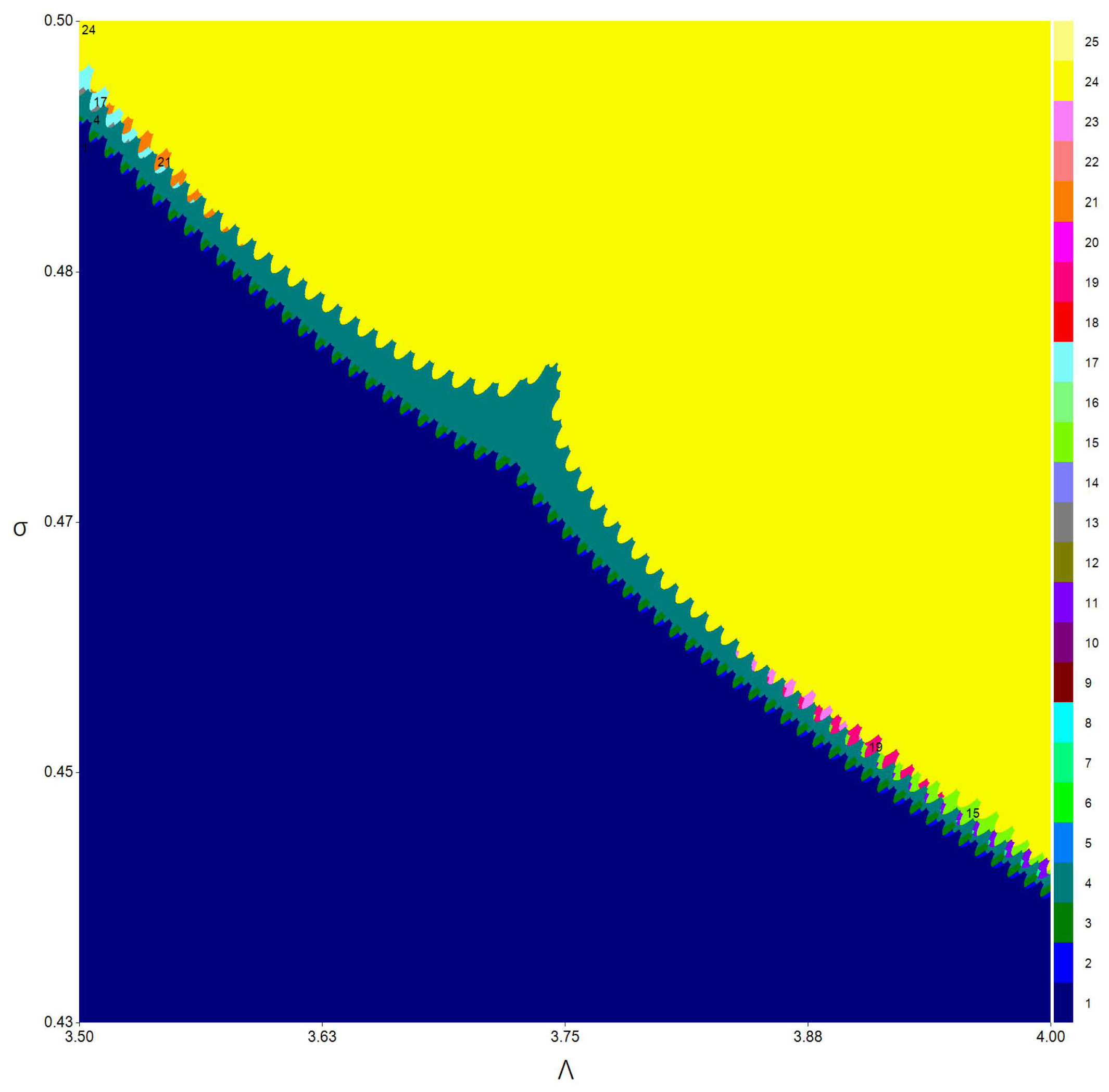
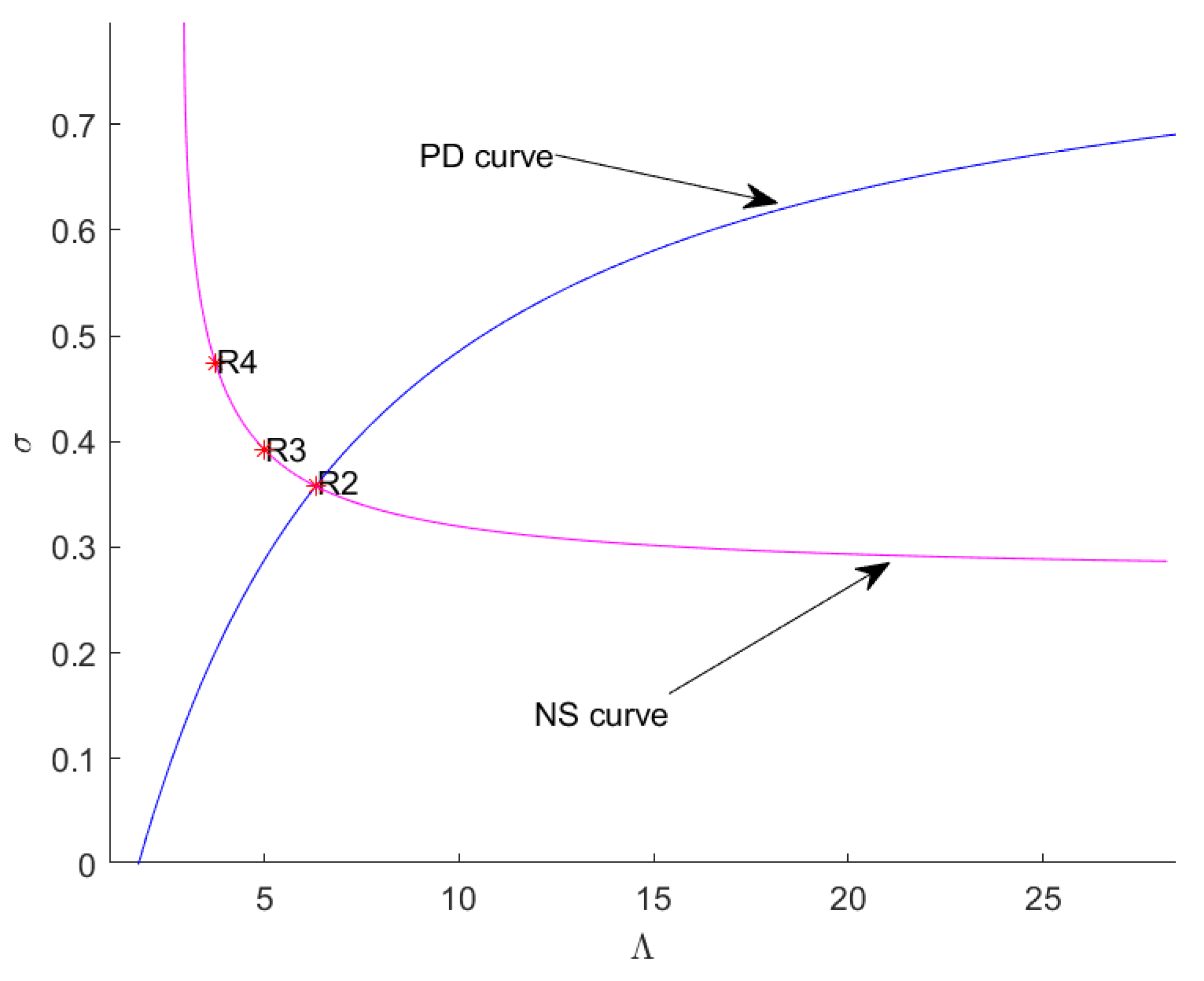
• The resonance 1:4 bifurcation occurs at ${\mathcal{E}}_{*}$ for $\Lambda =3.741538$ and $\sigma =0.474818$ where ${\Pi }_{R_4,*}=9.557396\times {10}^{-2}-2.715659\times {10}^{-1}i$. If we compute the convergent orbits from initial point $(S,I)=(3.1984,3.5905)$ with respect to $\Lambda$ and $\sigma ,$ a two-dimensional bifurcation diagram in the neighborhood of the R4 point can be displayed with the period number of the corresponding orbits [28,29]; see Figure 4. In addition to the parameter region with a period-4 cycle, there also exist regions with fixed points—period-2, -11, -15, -17, -19 and -21 cycles—to show complex periodic dynamics. Here, a stable period-4 cycle occurs when $(\Lambda ,\sigma )=(3.75,0.45)$ and one of a period-4 cycle is (3.092783505154633,3.762886597938157).
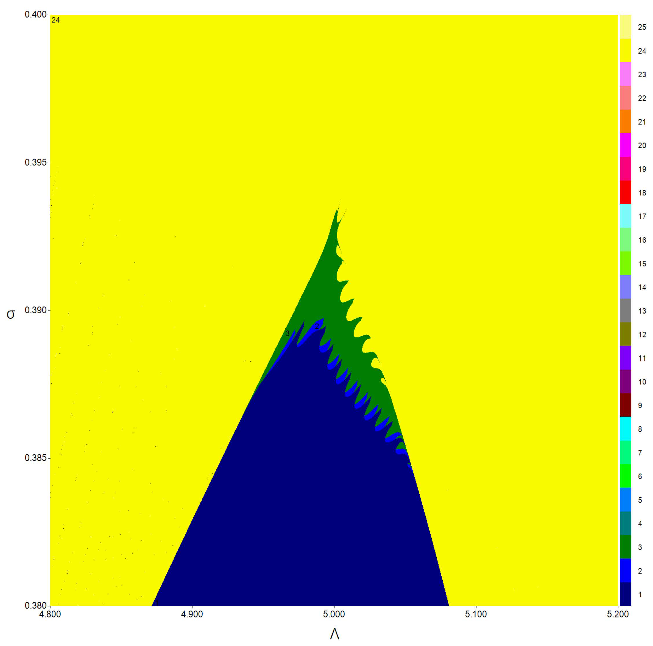
• The resonance 1:3 bifurcation occurs at ${\mathcal{E}}_{*}$ for $\Lambda =4.999711$ and $\sigma =0.392641$ where $\Re \left(\frac{3}{4}(2e^{i\frac{4\pi }{3}}{\upsilon }_{R_3,*}-|{\gamma }_{R_3,*}{|}^2)\right)=4.403109\times {10}^{-2}$. If we compute the convergent orbits from initial point $(S,I)=(2.8495,5.9841)$ with respect to $\Lambda$ and $\sigma ,$ a two-dimensional bifurcation diagram in the neighborhood of the R3 point can be displayed with the period number of the corresponding orbits; see Figure 5. In addition to the parameter region with a period-3 cycle, there only exist regions with fixed points and a period-2 cycle. Here, a stable period-3 cycle occurs when $(\Lambda ,\sigma )=(4.9,0.38)$ and one of the period-3 cycle is (2.796052631578960,5.972329721362207).
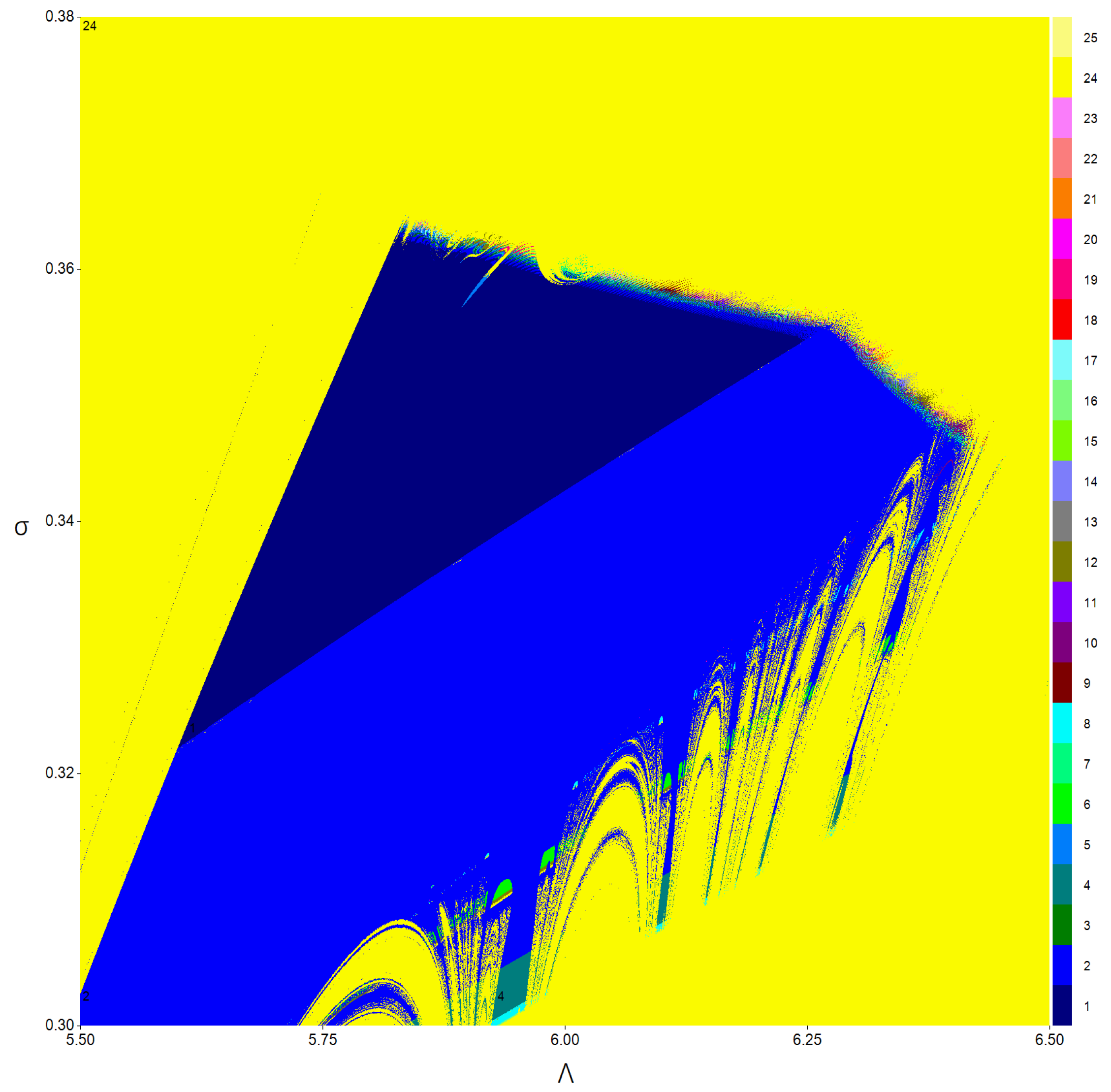
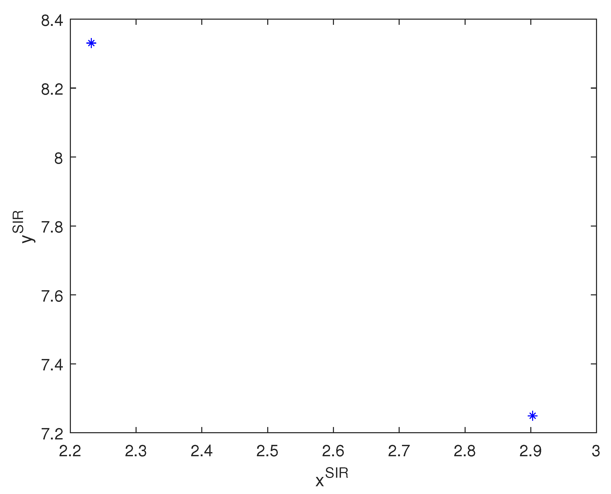
• The resonance 1:2 bifurcation occurs at ${\mathcal{E}}_{*}$ for $\Lambda =6.321289$ and $\sigma =0.357760$ where ${\upsilon }_{R_2,*}=-1.731233\times {10}^{-1}$ and ${\gamma }_{R_2,*}=1.575539\times {10}^{-2}$. If we compute the convergent orbits from initial point $(S,I)=(2.7021,8.3779)$ with respect to $\Lambda$ and $\sigma ,$ a two-dimensional bifurcation diagram in the neighborhood of the R2 point can be displayed with the period number of the corresponding orbits; see Figure 6. In addition to the parameter region with a period-2 cycle, there only exist regions with fixed points and period-4, -6, and -8 cycles. Here, a stable period-2 cycle occurs when $(\Lambda ,\sigma )=(5.6,0.32)$ and one of the period-2 cycles is (2.232027014018290,8.330641606985276); see Figure 7.

The stability region of ${\mathcal{E}}_{*}$ in space $(\Lambda ,\sigma )$ and the bifurcation curves of the flip and the Neimark–Sacker are shown in Figure 8 and Figure 9. Figure 9 confirms the results of Theorems 7–9.

The bifurcation curves of the second and third iterates of (3) are presented in Figure 10a,b.

6. Discussion

We presented a discrete-time $SIR$ epidemic model with detailed complex dynamics in this study. Using analytical and numerical methods, we analyzed the bifurcation of the boundary and positive fixed points ${\mathcal{E}}_0^{SIR}$ and ${\mathcal{E}}_{*}^{SIR}$.

By incorporating the Neimark–Sacker bifurcation into the model, we can infer that susceptible and infective individuals can fluctuate around some mean values of the population recruitment rate, and these fluctuations remain stable as well as constant if ${\upsilon }_{NS,*}<0$. According to biological theory, an invariant curve bifurcates from a fixed point, which allows susceptible and infected individuals to coexist and produce their densities. Periodic or quasi-periodic dynamics may be observed on an invariant curve. It appears that the susceptible and infected individuals change from one period to the next in this model based upon the period-doubling bifurcation. On the other hand, the strong resonances bifurcation of the model suggests susceptible and infected individuals coexist in stable high period cycles around some mean values of the rate of population recruitment rate and infection rate of infected individuals. Some two-dimensional bifurcation diagrams in the neighborhood of two-parameter bifurcation point are computed and displayed to show possible periodic dynamics.

7. Conclusions

The dynamics of a system can be identified and predicted using bifurcation theory. In this sense, bifurcation theory is an important branch of dynamical systems theory. In this paper, we provide a standard research format of bifurcation analysis. The existence and stability of fixed points are provided in Section 2. In Section 3 and Section 4, one-parameter bifurcations and two-parameter bifurcations are analyzed, respectively. Detailed instructions are given in Section 5 regarding the computation of fixed point curves. According to Section 3, Section 4 and Section 5, the numerical observations and the analytical predictions are in excellent agreement. Discussions are summarized in Section 6. Both analytical and numerical aspects of bifurcations are considered in dynamic models. Some methods are more efficient than others for studying bifurcations in each of these two aspects. The computation of the critical normal form coefficients is a very effective analytical method in bifurcation theory. One can see different kinds of methods employed in bifurcation analysis [30,31,32,33,34,35,36]. There are many dynamical systems that are prone to notice this method, discrete or continuous; see [37,38,39,40,41,42,43]. An analytical computation is performed in this paper, and the results are also validated numerically using MatcontM. More details can be found in Kuznetsov and Meijer (2005) [25] and Govaerts et al. (2007) [27]. The paper also provides a robust analytical and numerical method that can be applied to different discrete-time models.

References

1. Barrientos, P.G.; Rodríguez, J.Á.; Ruiz-Herrera, A. Chaotic dynamics in the seasonally forced SIR epidemic model. J. Math. Biol. 2017, 75, 1655–1668. [Google Scholar] [CrossRef] [PubMed]
2. Diedrichs, D.R.; Isihara, P.A.; Buursma, D.D. The schedule effect:can recurrent peak infections be reduced without vaccines, quarantines or school closings? Math. Biosci. 2014, 248, 46–53. [Google Scholar] [CrossRef]
3. Axelsen, J.B.; Yaari, R.; Grenfell, B.T.; Stone, L. Multiannual forecasting of seasonal influenza dynamics reveals climatic and evolutionary drivers. Proc. Natl. Acad. Sci. USA 2014, 111, 9538–9542. [Google Scholar] [CrossRef] [PubMed] [Green Version]
4. Dietz, K. The incidence of infectious diseases under the influence of seasonal fluctuations. In Mathematical Models in Medicine; Springer: Berlin/Heidelberg, Germany, 1976; pp. 1–15. [Google Scholar]
5. Aron, J.L.; Schwartz, I.B. Seasonality and period-doubling bifurcations in an epidemic model. J. Theor. Biol. 1984, 110, 665–679. [Google Scholar] [CrossRef]
6. Eskandari, Z.; Alidousti, J. Stability and codimension 2 bifurcations of a discrete time SIR model. J. Frankl. Inst. 2020, 357, 10937–10959. [Google Scholar] [CrossRef]
7. Li, X.; Wang, W. A discrete epidemic model with stage structure. Chaos Solitons Fractals 2005, 26, 947–958. [Google Scholar] [CrossRef]
8. Naik, P.A.; Zu, J.; Ghoreishi, M. Stability analysis and approximate solution of SIR epidemic model with Crowley-Martin type functional response and Holling type-II treatment rate by using homotopy analysis method. J. Appl. Anal. Comput. 2020, 10, 1482–1515. [Google Scholar]
9. Stone, L.; Olinky, R.; Huppert, A. Seasonal dynamics of recurrent epidemics. Nature 2007, 446, 533–536. [Google Scholar] [CrossRef]
10. Ghori, M.B.; Naik, P.A.; Zu, J.; Eskari, Z.; Naik, M. Global dynamics and bifurcation analysis of a fractional-order SEIR epidemic model with saturation incidence rate. Math. Methods Appl. Sci. 2022, 45, 1–33. [Google Scholar] [CrossRef]
11. Karaji, P.T.; Nyamoradi, N. Analysis of a fractional SIR model with general incidence function. Appl. Math. Lett. 2020, 108, 106499. [Google Scholar] [CrossRef]
12. Naik, P.A. Global dynamics of a fractional-order SIR epidemic model with memory. Int. J. Biomath. 2020, 13, 2050071. [Google Scholar] [CrossRef]
13. Zhang, Q.; Tang, B.; Tang, S. Vaccination threshold size and backward bifurcation of SIR model with state-dependent pulse control. J. Theor. Biol. 2018, 455, 75–85. [Google Scholar] [CrossRef] [PubMed]
14. BjØrnstad, O.N.; Finkenstädt, B.F.; Grenfell, B.T. Dynamics of measles epidemics: Estimating scaling of transmission rates using a time series SIR model. Ecol. Monogr. 2002, 72, 169–184. [Google Scholar]
15. Olsen, L.F.; Schaffer, W.M. Chaos versus noisy periodicity: Alternative hypotheses for childhood epidemics. Science 1990, 249, 499–504. [Google Scholar] [CrossRef]
16. Augeraud-Véron, E.; Sari, N. Seasonal dynamics in an SIR epidemic system. J. Math. Biol. 2014, 68, 701–725. [Google Scholar]
17. Duarte, J.; Januário, C.; Martins, N.; Rogovchenko, S.; Rogovchenko, Y. Chaos analysis and explicit series solutions to the seasonally forced SIR epidemic model. J. Math. Biol. 2019, 78, 2235–2258. [Google Scholar] [CrossRef]
18. Kermack, W.O.; McKendrick, A.G. A contribution to the mathematical theory of epidemics. Proc. R. Soc. Lond. Ser. Contain. Pap. Math. Phys. Character 1927, 115, 700–721. [Google Scholar]
19. Hethcote, H.W. The mathematics of infectious diseases. SIAM Rev. 2000, 42, 599–653. [Google Scholar] [CrossRef] [Green Version]
20. Akrami, M.H.; Atabaigi, A. Hopf and forward bifurcation of an integer and fractional-order SIR epidemic model with logistic growth of the susceptible individuals. J. Appl. Math. Comput. 2020, 64, 615–633. [Google Scholar] [CrossRef]
21. Hu, Z.; Teng, Z.; Zhang, L. Stability and bifurcation analysis in a discrete SIR epidemic model. Math. Comput. Simul. 2014, 97, 80–93. [Google Scholar] [CrossRef]
22. Liu, X.; Xiao, D. Complex dynamic behaviors of a discrete-time predator-prey system. Chaos Solitons Fractals 2007, 32, 80–94. [Google Scholar] [CrossRef]
23. He, Z.; Lai, X. Bifurcation and chaotic behavior of a discrete-time predator-prey system. Nonlinear Anal. Real World Appl. 2011, 12, 403–417. [Google Scholar] [CrossRef]
24. Kuznetsov, Y.A. Elements of Applied Bifurcation Theory; Springer Science & Business Media: Berlin/Heidelberg, Germany, 2013; Volume 112. [Google Scholar]
25. Kuznetsov, Y.A.; Meijer, H.G. Numerical normal forms for codim 2 bifurcations of fixed points with at most two critical eigenvalues. Siam J. Sci. Comput. 2005, 26, 1932–1954. [Google Scholar] [CrossRef] [Green Version]
26. Kuznetsov, Y.A.; Meijer, H.G. Numerical Bifurcation Analysis of Maps: From Theory to Software; Cambridge University Press: Cambridge, UK, 2019. [Google Scholar]
27. Govaerts, W.; Ghaziani, R.K.; Kuznetsov, Y.A.; Meijer, H.G. Numerical methods for two-parameter local bifurcation analysis of maps. Siam J. Sci. Comput. 2007, 29, 2644–2667. [Google Scholar] [CrossRef]
28. Li, B.; Liang, H.J.; He, Q.Z. Multiple and generic bifurcation analysis of a discrete Hindmarsh-Rose model. Chaos Solitons Fractals 2021, 146, 110856. [Google Scholar] [CrossRef]
29. Li, B.; Liang, H.J.; Shi, L.; He, Q.Z. Complex dynamics of Kopel model with nonsymmetric response between oligopolists. Chaos Solitons Fractals 2022, 156, 111860. [Google Scholar] [CrossRef]
30. Li, X.L.; Su, L. A heterogeneous duopoly game under an isoelastic demand and diseconomies of scale. Fractal Fract. 2022, 6, 459. [Google Scholar] [CrossRef]
31. Jiang, X.W.; Chen, C.; Zhang, X.H.; Chi, M.; Yan, H. Bifurcation and chaos analysis for a discrete ecological developmental systems. Nonlinear Dyn. 2021, 104, 4671–4680. [Google Scholar] [CrossRef]
32. Rahmi, E.; Darti, I.; Suryanto, A.; Trisilowati. A Modified Leslie–Gower Model Incorporating Beddington–DeAngelis Functional Response, Double Allee Effect and Memory Effect. Fractal Fract. 2021, 5, 84. [Google Scholar] [CrossRef]
33. Li, P.; Yan, J.; Xu, C.; Gao, R.; Li, Y. Understanding Dynamics and Bifurcation Control Mechanism for a Fractional-Order Delayed Duopoly Game Model in Insurance Market. Fractal Fract. 2022, 6, 270. [Google Scholar] [CrossRef]
34. Wang, H.; Ke, G.; Pan, J.; Hu, F.; Fan, H. Multitudinous potential hidden Lorenz-like attractors coined. Eur. Phys. J.-Spec. Top. 2022, 231, 359–368. [Google Scholar] [CrossRef]
35. Wang, N.; Zhang, G.S.; Kuznetsov, N.V.; Bao, H. Hidden attractors and multistability in a modified Chua’s circuit. Commun. Nonlinear Sci. Numer. Simul. 2021, 92, 105494. [Google Scholar] [CrossRef]
36. Ali, M.S.; Narayanan, G.; Shekher, V.; Alsulami, H.; Saeed, T. Dynamic stability analysis of stochastic fractional-order memristor fuzzy BAM neural networks with delay and leakage terms. Appl. Math. Comput. 2020, 369, 124896. [Google Scholar]
37. Eskandari, Z.; Alidousti, J.; Avazzadeh, Z.; Ghaziani, R.K. Dynamics and bifurcations of a discrete time neural network with self connection. Eur. J. Control 2022, 66, 100642. [Google Scholar] [CrossRef]
38. Eskandari, Z.; Alidousti, J.; Avazzadeh, Z.; Machado, J.T. Dynamics and bifurcations of a discrete-time prey-predator model with Allee effect on the prey population. Ecol. Complex. 2021, 48, 100962. [Google Scholar] [CrossRef]
39. Eskandari, Z.; Avazzadeh, Z.; Ghaziani, R.K. Complex dynamics of a Kaldor model of business cycle with discrete-time. Chaos, Solitons Fractals 2022, 157, 111863. [Google Scholar] [CrossRef]
40. Eskandari, Z.; Avazzadeh, Z.; Khoshsiar Ghaziani, R.; Li, B. Dynamics and bifurcations of a discrete-time Lotka-Volterra model using non-standard finite difference discretization method. Math. Methods Appl. Sci. 2022. [Google Scholar] [CrossRef]
41. Xiao, Y.; Zhang, S.G.; Peng, Y. Dynamic investigations in a Stackelberg model with differentiated products and bounded rationality. J. Comput. Appl. Math. 2022, 414, 114409. [Google Scholar] [CrossRef]
42. Barge, H.; Sanjurjo, J.M.R. Higher dimensional topology and generalized Hopf bifurcations for discrete dynamical systems. Discret. Contin. Dyn. Syst. 2021, 42, 2585–2601. [Google Scholar] [CrossRef]
43. Tassaddiq, A.; Shabbir, M.S.; Din, Q.; Naaz, H. Discretization, Bifurcation, and Control for a Class of Predator-Prey Interactions. Fractal Fract. 2020, 6, 31. [Google Scholar] [CrossRef]
Figure 1. The stability region of E 0 in space ( Λ , σ ) .
Fractalfract 06 00659 g001
Figure 2. Phase portraits of model (3). (a) A stable fixed point for Λ = 3.75 . (b) The phase portrait of model (3) for Λ = 3.780 (c) A closed invariant curve for Λ = 3.78404 . (d) The broken invariant closed curve for Λ = 3.788 .
Fractalfract 06 00659 g002
Figure 3. Bifurcation diagram of model (3) in ( Λ , S ) -plane.
Fractalfract 06 00659 g003
Figure 4. Two-dimensional bifurcation diagram of (3) in the neighborhood of the R 4 point.
Fractalfract 06 00659 g004
Figure 5. Two-dimensional bifurcation diagram of (3) in the neighborhood of the R 3 point.
Fractalfract 06 00659 g005
Figure 6. Two-dimensional bifurcation diagram of (3) in the neighborhood of the R 2 point.
Fractalfract 06 00659 g006
Figure 7. Stable period-2 cycle.
Fractalfract 06 00659 g007
Figure 8. The stability region of E * in space ( Λ , σ ) .
Fractalfract 06 00659 g008
Figure 9. The bifurcation diagram of (3) near E * .
Fractalfract 06 00659 g009
Figure 10. (a) The N S 2 curve. (b) The N S 3 curve.
Fractalfract 06 00659 g010