Compound Adaptive Fuzzy Synchronization Controller Design for Uncertain Fractional-Order Chaotic Systems

Abstract

In this paper, the synchronization of two fractional-order chaotic systems with uncertainties and external disturbances is considered. A fuzzy logic system is utilized to estimate uncertain nonlinearity, and its estimation accuracy is improved by constructing a series-parallel model. A disturbance observer is implemented to estimate bounded disturbance. To solve the “explosion of complexity” problem in the backstepping scheme, fractional-order command filters are employed to estimate virtual control inputs and their derivatives, and error compensation signals are devised to reduce filtering errors. Based on the fractional-order Lyapurov criterion, the proposed compound adaptive fuzzy backstepping control strategy can guarantee that the synchronization error converges to a small neighborhood of the origin. At last, the validity of the proposed control strategy is verified via a numerical simulation.

1. Introduction

Fractional calculus has been developed for over three centuries, which can be seen as an extension of ordinary calculus. It plays an important role in dealing with the control problem of non-integer order systems, which has received extensive attention due to its fascinating properties and potential application values. Over the past few decades, it has been discovered that in some real-world systems related to time series, compared with integer-order systems, fractional-order systems have better modeling accuracy due to the memory and inheritance of fractional calculus, such as financial systems [1], viscoelastic systems [2], dielectric polarization [3], and electrode–electrolyte polarization [4].

Nowadays, some studies have indicated that a lot of fractional-order systems exhibit chaotic phenomena, which is nonlinearity with complexity, randomness, unpredictability and extreme sensitivity to initial values [5,6,7,8], and has great application value in secure communication [9], signal processing, mathematical biology and machinery [5], etc. So far, scholars have proposed various control strategies to achieve the synchronization of fractional-order chaotic systems (FOCSs), e.g., sliding mode control [10], adaptive control [11], backstepping control [12], etc. Among them, backstepping control is an effective and commonly utilized method to realize the synchronization of FOCSs with the form of strict feedback. On the other hand, in actual modeling, due to the measurement errors, parameter uncertainties, external disturbances and other factors, the uncertain items often appear in the FOCSs which will affect the synchronization performance. Therefore, an ingenious idea is to combine backstepping control with function estimation techniques to handle its uncertainties so as to achieve the control objective. In [13], Ha et al. devised an adaptive fuzzy backstepping control (AFBC) method to realize the synchronization of FOCSs. Simultaneously, the fractional derivative of the virtual control function was regarded as a part of the uncertainties and was estimated by the fuzzy logic system (FLS) so as to enhance the performance of synchronization and reduce the amount of calculation. In [14], a backstepping sliding mode control scheme was devised for a typical fractional-order quadrotor unmanned aerial vehicle, which can reduce the chattering phenomenon and improve the response and convergence speeds. In [15], a hybrid control method combining AFBC and sliding mode control was adopted to achieve fast and high-precision control of nonlinear fully actuated and underactuated mechanical systems in the presence of uncertainties. It is worth emphasizing that the backstepping control schemes utilized in the above literature can effectively achieve the control objectives, but the disadvantage of these schemes is that they will lead to an increase in computational complexity due to repeated differentiation of virtual control inputs. Therefore, how to devise a suitable method to reduce the computational complexity is meaningful and necessary work.

In recent years, some scholars have introduced the fractional-order command filter to estimate the derivatives of virtual control inputs to settle the “explosion of complexity” problem, and some interesting research results have been realized. In [16], Ha et al. devised an AFBC method to achieve the control objective, and adopted a fractional-order command filter to approximate the derivative of the virtual input. Simultaneously, an error compensation mechanism was utilized to handle errors generated in the filtering process. In [17], Han et al. devised an AFBC scheme with a fractional-order command filter for fractional-order systems. Among them, the fractional-order command filter was employed to eliminate the differential expansion of the backstepping controller, and the sliding mode controller was utilized to enhance the robustness of the system. In [18], a method combining AFBC and finite-time sliding mode control was employed for fractional-order systems with actuator faults, which not only exhibits superior robustness, but also helps to complete all the required tracking control targets in some finite time. It is noted that the filter used in the above literature has a strong approximation effect on the virtual control input and its derivative, and finally achieved a good control effect, but the discussion on the estimation accuracy of parameters is rare. However, in many practical systems, such as navigation systems and industrial lockstitch machine systems, the requirements for parameter accuracy are very high. Therefore, how to improve the estimation accuracy of parameters deserves further consideration.

In order to solve the above problem, a natural idea is to increase number of rules or neural nodes when estimating uncertain terms by FLSs or neural networks, but this method will increase the computational burden. Therefore, to avoid this situation, a series-parallel model is introduced, whose main idea is to construct a prediction error as an additional feedback term for the adaptive law. In [19], Liu et al. exploited a compound learning sliding mode control strategy for triangular fractional-order systems, in which a prediction error is defined and combined with a tracking error to construct a compound learning law to improve the estimation accuracy of the parameters. In [20], Zhou et al. devised a T-S fuzzy-based compound learning control strategy to synchronize two FOCSs with both uncertain parameters and time-varying delays. Furthermore, the proposed interval excitation condition can ensure a fast convergence of the parameters. In [21], Han et al. utilized online recorded data and instantaneous data to define a prediction error and combined a synchronization error to build a series-parallel model, and the proposed composite learning sliding mode control scheme ensured that the synchronization error asymptotically tends to zero. However, note that the disturbance is considered in the above literature and handled by an adaptive law, but this method will produce a disturbance error and have a negative impact on the control performance.

As far as we know, an effective solution to deal with the effects of disturbances is to devise a disturbance observer (DOB). In [22], Mofid et al. combined a DOB with an adaptive sliding mode control scheme to achieve a rapid response for the synchronization of three-dimensional FOCSs. In [23], Li et al. adopted a saturation control scheme to control a double-pendulum offshore crane subjected to matching disturbance, and constructed a fractional-order DOB to eliminate the effect of the matching disturbance. In [24], Guha et al. developed a DOB to estimate disturbance in an endogenous or exogenous system to accelerate dynamic response with minimal flutter, and utilized the Mittag–Leffler stability theorem to ensure the finite time convergence of disturbance error. The above literature provides a lot of outstanding solutions for dealing with disturbances. How to combine the DOB with the backstepping control technology to handle the synchronous control of FOCSs deserves further study.

Inspired by the above discussion, this paper studies the synchronization of FOCSs with uncertainties and external disturbances based on compound AFBC technology. First, FLSs are utilized to estimate uncertain terms, and series-parallel models are constructed to enhance their estimation accuracy, while DOBs are devised to estimate disturbances. For two different chaotic systems, the main objective of this paper is to design a compound adaptive fuzzy controller to ensure that synchronization errors converge to a small neighborhood of the origin and all signals are bounded. Simultaneously, the effectiveness of the proposed method is demonstrated by the Lyapunov stability theory. Finally, the contributions of this article are shown below. (1) It is difficult to achieve a very ideal effect by using traditional fuzzy methods to approximate uncertain nonlinear terms or parameters in the system. However, in many practical systems, the requirement of parameter accuracy is very high. The series parallel model proposed in this paper can effectively improve the approximation accuracy without increasing the number of fuzzy rules. (2) Compared with the traditional DOB, the proposed DOB in this paper adds a prediction error as a feedback term to further improve the observation accuracy.

Here is the remaining part of this study. In Section 2, the notation and preliminaries are displayed. In Section 3, the master–slave systems are introduced, and DOBs and adaptive fuzzy controllers are designed, while stability analysis is performed by using the Lyapunov method. In Section 4, a simulation example is employed to check the feasibility and validity of this means. Furthermore, the conclusion is given in Section 5.

2. Preliminaries

2.1. Definitions and Lemmas

In this part, several fundamental definitions and lemmas with respect to fractional-order integrals and derivatives will be presented, which are useful for stability analysis.

Definition 1 

([25]). The fractional integral with order $\vartheta \in (0,1)$ is defined as

$$\begin{array}{c}{\mathcal{I}}^{\vartheta }f\left(t\right)=\frac{1}{\mathsf{\Gamma }\left(\vartheta \right)}{\int }_{t_0}^t\frac{f\left(\varrho \right)}{{(t-\varrho )}^{1-\vartheta }}d\varrho ,\end{array}$$

(1)

where $t\ge t_0$, $\mathsf{\Gamma }\left(\vartheta \right)={\int }_0^{\infty }{e}^{-t}{t}^{\vartheta -1}dt$.

In this paper, we mainly consider the Caputo fractional derivative, owing to the fact that its initial conditions for fractional differential equations possess the identical physical meaning with the integer-order one.

Definition 2 

([26]). The Caputo fractional derivative with order $\vartheta \in (0,1)$ is described as

$$\begin{array}{c}{}^c{\mathcal{D}}^{\vartheta }f\left(t\right)=\frac{1}{\mathsf{\Gamma }(1-\vartheta )}{\int }_{t_0}^t\frac{f^{\prime }\left(\varrho \right)}{{(t-\varrho )}^{\vartheta }}d\varrho ,\end{array}$$

(2)

where $f\left(t\right)\in {\mathbb{C}}^n\left(\right[t_0$, $+\infty ]$, $\mathbb{R})$. Hereafter, ${\mathcal{D}}^{\vartheta }$ represents ${}^c{\mathcal{D}}^{\vartheta }$ for convenience.

Definition 3 

([27]). The Mittag–Leffler function is

$$E_{\iota ,\nu }\left(\varphi \right)=\sum _{\kappa =0}^{\infty }\frac{{\varphi }^{\kappa }}{\mathsf{\Gamma }(\iota \kappa +\nu )},$$

(3)

where $\iota ,\nu \in {\mathbb{R}}^{+}$, and $\varphi \in \mathbb{C}$, and its Laplace transformation is

$$\mathcal{L}\left\{t^{\nu -1}{E}_{\iota ,\nu }(-c{t}^{\iota })\right\}=\frac{s^{\iota -\nu }}{s^{\iota }+c}.$$

(4)

Lemma 1 

([28]). Let $\varpi \left(t\right)\in \mathbb{R}$ be a real-valued continuous differentiable vector function, then we have

$$\begin{array}{c}\frac{1}{2}{\mathcal{D}}^{\vartheta }{\varpi }^T\varpi \le {\varpi }^T{\mathcal{D}}^{\vartheta }\varpi \forall \vartheta \in (0,1],t\ge 0.\end{array}$$

(5)

Lemma 2 

([29]). (Yong’s Inequality) For $\forall a,b\ge 0$, the following inequality holds:

$$\begin{array}{c}ab\le \frac{a^p}{p}+\frac{b^q}{q}.\end{array}$$

(6)

Lemma 3 

([30]). For $\nu \in \mathbb{C}$, $0<\iota <1$ and $\frac{\pi \iota }{2}<\phi <min\left\{\pi ,\pi \iota \right\}$, we can obtain

$$E_{\iota ,\nu }\left(\varphi \right)=-\sum _{j=1}^n\frac{1}{\mathsf{\Gamma }(\nu -\iota j){\varphi }^j}+o\left(\frac{1}{{\left|\varphi \right|}^{n+1}}\right),$$

(7)

when $n\ge 1$, $\left|\varphi \right|\to \infty$, $\phi \le \left|arg\right(\varphi \left)\right|\le \pi$.

Lemma 4 

([31]). Supposing σ is a normal number, the following holds:

$$\begin{array}{c}\left|\eta \right|-\eta tanh\left(\frac{\eta }{\sigma }\right)\le 0.2785\sigma ={\sigma }^{\prime }.\end{array}$$

(8)

Lemma 5 

([31]). Suppose that $0<\upsilon <2$ and $\varsigma \in \mathbb{R}$. If there exists $\zeta \in {\mathbb{R}}^{+}$, such that $\left(\frac{\pi \upsilon }{2}\right)<\zeta \le min\left\{\pi ,\pi \upsilon \right\}$, then we have

$$|E_{\upsilon ,\varsigma }\left(\varphi \right)|\le \frac{p}{1+\left|\varphi \right|},$$

(9)

where $p\in {\mathbb{R}}^{+}$, $\zeta \le \left|arg\right(\varphi \left)\right|\le \pi$.

2.2. The Fuzzy Logic System

In the next part, in order to estimate the uncertainty, an FLS is required and characterized as below.

The ith rule is portrayed as below: ${\mathbb{R}}^{\left(i\right)}$: if ${\mu }_1$ is ${\mathsf{{\rm Y}}}_1^i$, …, ${\mu }_n$ is ${\mathsf{{\rm Y}}}_n^i$, then $\widehat{\mathsf{\Phi }}$ is ${\mathsf{\Xi }}^i$, where ${\mathsf{{\rm Y}}}_1^i,\dots$, ${\mathsf{{\rm Y}}}_n^i$ are fuzzy sets and $\widehat{\mathsf{\Phi }}$ is the output. Through taking advantage of the defuzzification, the FLS output can be manifested as shown below:

$$\begin{array}{cc}\hfill \widehat{\mathsf{\Phi }}\left(\mu \right)& =\frac{{\sum }_{i=1}^q{\rho }_i\left({\prod }_{j=1}^n{ð}_{{\mathsf{{\rm Y}}}_j^i}\left({\mu }_j\right)\right)}{{\sum }_{i=1}^q\left({\prod }_{j=1}^n{ð}_{{\mathsf{{\rm Y}}}_j^i}\left({\mu }_j\right)\right)}\hfill \\ \hfill & ={\rho }^T\xi \left(\mu \right),\hfill \end{array}$$

(10)

where $\widehat{\mathsf{\Phi }}\left(\mu \right)$ is the approximation of the $\mathsf{\Phi }\left(\mu \right)$, ${ð}_{{\mathsf{{\rm Y}}}_j^i}\left({\mu }_j\right)$ is the degree of membership of ${\mu }_j$ to ${\mathsf{{\rm Y}}}_j^i$, q is the amount of fuzzy rules, $\rho ={[{\rho }_1,\dots ,{\rho }_q]}^T$ is the adjustable parameter vector, and $\xi ={[{\xi }_1,\dots ,{\xi }_q]}^T$, where

$${\xi }_i\left(\mu \right)=\frac{{\prod }_{j=1}^n{ð}_{{\mathsf{{\rm Y}}}_j^i}\left({\mu }_j\right)}{{\sum }_{i=1}^q\left({\prod }_{j=1}^n{ð}_{{\mathsf{{\rm Y}}}_j^i}\left({\mu }_j\right)\right)}$$

is the fuzzy basis function (FBF), assuming that the picked FBFs have at least one active rule count, i.e., ${\sum }_{i=1}^q\left({\prod }_{j=1}^n{ð}_{{\mathsf{{\rm Y}}}_j^i}\left({\mu }_j\right)\right)>0$.

Later, the unknown function ${\mathsf{\Phi }}_i\left(\mu \right)$ can be estimated by employing (10):

$$\begin{array}{c}{\mathsf{\Phi }}_i\left({\mu }_i\right)={{\rho }_i^{*}}^T{\xi }_i\left({\mu }_i\right)+{\epsilon }_i\left({\mu }_i\right),\end{array}$$

(11)

where ${\epsilon }_i\left({\mu }_i\right)$ is the optimal estimation error, and the optimal estimation of ${\rho }_i$ can be described as

$${\rho }_i^{*}=arg\underset{{\rho }_i}{min}\left[\underset{{\mu }_i\in {\Omega }_{{\mu }_i}}{sup}|{\mathsf{\Phi }}_i\left({\mu }_i\right)-{\widehat{\mathsf{\Phi }}}_i({\mu }_i,{\rho }_i)|\right],$$

(12)

and note that the vector ${\rho }_i^{*}$ is only utilized for stability analysis. It is not necessary to calculate its specific values in the implementation process.

Therefore, from (10) and (11), we have

$$\begin{array}{cc}\hfill {\widehat{\mathsf{\Phi }}}_i({\mu }_i,{\rho }_i)-{\mathsf{\Phi }}_i\left({\mu }_i\right)& ={\widehat{\mathsf{\Phi }}}_i({\mu }_i,{\rho }_i)-{\widehat{\mathsf{\Phi }}}_i({\mu }_i,{\rho }_i^{*})+{\widehat{\mathsf{\Phi }}}_i({\mu }_i,{\rho }_i^{*})-{\mathsf{\Phi }}_i\left({\mu }_i\right)\hfill \\ ={\rho }_i^T{\xi }_i\left({\mu }_i\right)-{{\rho }_i^{*}}^T{\xi }_i\left({\mu }_i\right)+{\epsilon }_i\left({\mu }_i\right)\hfill \\ ={\tilde{\rho }}_i^T{\xi }_i\left({\mu }_i\right)+{\epsilon }_i\left({\mu }_i\right),\hfill \end{array}$$

(13)

where ${\tilde{\rho }}_i={\rho }_i-{\rho }_i^{*}$, and ${\epsilon }_i\left({\mu }_i\right)={\widehat{\mathsf{\Phi }}}_i({\mu }_i,{\rho }_i^{*})-{\mathsf{\Phi }}_i\left({\mu }_i\right)$.

Remark 1. 

Obviously, the FLS (10) is greatly universally employed in control applications. According to the general approximation outcomes, the FLS (10) can approximate any nonlinear smooth function Φ with arbitrary precision in a compact operation space, presuming that the construction of the FLS (10), i.e., membership function parameters and number of rules, is correctly predesigned by the designer and the parameter ρ is defined by the learning algorithm.

3. Main Results

3.1. System Description

Consider a class of uncertain FOCSs portrayed as below.

The master system is

$$\left\{\begin{array}{c}{\mathcal{D}}^{\vartheta }{x}_i\left(t\right)=x_{i+1}\left(t\right)+f_i\left({\overline{x}}_i\left(t\right)\right),(i=1,\cdots ,n-1),\hfill \\ {\mathcal{D}}^{\vartheta }{x}_n\left(t\right)=f_n\left({\overline{x}}_n\left(t\right)\right),\hfill \end{array}\right.$$

(14)

where $x_i\in \mathbb{R}$ is the measurable state vector, ${\overline{x}}_i={[x_1,x_2,\cdots ,x_i]}^T\in {\mathbb{R}}^i$, and $f_i\left({\overline{x}}_i\right)\in \mathbb{R}$ is an unknown smooth function.

The slave system is

$$\left\{\begin{array}{c}{\mathcal{D}}^{\vartheta }{y}_i\left(t\right)=y_{i+1}\left(t\right)+g_i\left({\overline{y}}_i\left(t\right)\right)+{\gamma }_i\left(t\right),(i=1,\cdots ,n-1),\hfill \\ {\mathcal{D}}^{\vartheta }{y}_n\left(t\right)=g_n\left({\overline{y}}_n\left(t\right)\right)+u\left(t\right)+{\gamma }_n\left(t\right),\hfill \end{array}\right.$$

(15)

where $y_i\in \mathbb{R}$ is the measurable state vector, ${\overline{y}}_i={[y_1,y_2,\cdots ,y_i]}^T\in {\mathbb{R}}^i$, and $g_i\left({\overline{y}}_i\right)\in \mathbb{R}$ is an unknown smooth function, $\gamma \left(t\right)={[{\gamma }_1,\dots ,{\gamma }_n]}^T$ is an unknown disturbance vector, and $u={[u_1,\dots ,u_n]}^T\in {\mathbb{R}}^n$ represents the control input vector.

From (14) and (15), the error system can be characterized as follows:

$$\left\{\begin{array}{c}{\mathcal{D}}^{\vartheta }{e}_i\left(t\right)=e_{i+1}\left(t\right)+{\mathsf{\Phi }}_i({\overline{x}}_i,{\overline{y}}_i)+{\gamma }_i\left(t\right),\hfill \\ {\mathcal{D}}^{\vartheta }{e}_n\left(t\right)={\mathsf{\Phi }}_n({\overline{x}}_n,{\overline{y}}_n)+u\left(t\right)+{\gamma }_n\left(t\right),\hfill \end{array}\right.$$

(16)

where $e_{i+1}\left(t\right)=y_{i+1}-x_{i+1}$, and ${\mathsf{\Phi }}_i({\overline{x}}_i,{\overline{y}}_i)=g_i\left({\overline{y}}_i\left(t\right)\right)-f_i\left({\overline{x}}_i\left(t\right)\right)$. Hereafter, we will replace ${\mathsf{\Phi }}_i({\overline{x}}_i,{\overline{y}}_i)$ with ${\mathsf{\Phi }}_i\left({\mu }_i\right)$ for convenience.

Note that the unknown function ${\mathsf{\Phi }}_i\left({\mu }_i\right)$ can be directly estimated by the FLS (10), but it is difficult to obtain satisfactory estimation accuracy without increasing the number of fuzzy rules. Thus, to settle this problem, a series-parallel model is presented below:

$$\left\{\begin{array}{c}{\mathcal{D}}^{\vartheta }{\widehat{e}}_1={\widehat{e}}_2\left(t\right)+{\widehat{\mathsf{\Phi }}}_1({\mu }_1,{\rho }_1)+k_1{\tilde{e}}_1+{\widehat{\gamma }}_1,\hfill \\ {\mathcal{D}}^{\vartheta }{\widehat{e}}_i={\widehat{e}}_{i+1}\left(t\right)+{\widehat{\mathsf{\Phi }}}_i({\mu }_i,{\rho }_i)+k_i{\tilde{e}}_i+\frac{{\beta }_i}{{\beta }_{i-1}}{\tilde{e}}_{i-1}+{\widehat{\gamma }}_i,\hfill \\ {\mathcal{D}}^{\vartheta }{\widehat{e}}_n={\widehat{\mathsf{\Phi }}}_n({\mu }_n,{\rho }_n)+k_n{\tilde{e}}_n+\frac{{\beta }_n}{{\beta }_{n-1}}{\tilde{e}}_{n-1}+{\widehat{\gamma }}_n,\hfill \end{array}\right.$$

(17)

where $k_i\in {\mathbb{R}}^{+}$, and the prediction error is ${\tilde{e}}_i=e_i-{\widehat{e}}_i$.

3.2. Design of the Disturbance Observer

As we all know, unknown external disturbances often appear in real-world systems, which will affect the performance of the system. Therefore, immediately after, in order to estimate unknown disturbances of the slave system, DOBs will be devised.

To facilitate the design of DOBs, auxiliary variables are brought by

$$\left\{\begin{array}{c}{Q}_i\left(t\right)={\delta }_i{e}_i\left(t\right)-{\gamma }_i\left(t\right),\hfill \\ Q_n\left(t\right)={\delta }_n{e}_n\left(t\right)-{\gamma }_n\left(t\right).\hfill \end{array}\right.$$

(18)

From (16) and (18), the fractional derivative of $Q_i\left(t\right)$ can be obtained as

$$\begin{array}{cc}\hfill {\mathcal{D}}^{\vartheta }{Q}_i& ={\delta }_i{\mathcal{D}}^{\vartheta }{e}_i-{\mathcal{D}}^{\vartheta }{\gamma }_i\hfill \\ & ={\delta }_i(e_{i+1}+{\mathsf{\Phi }}_i\left({\mu }_i\right)+{\gamma }_i)-{\mathcal{D}}^{\vartheta }{\gamma }_i\hfill \\ & ={\delta }_i{e}_{i+1}+{\delta }_i{\mathsf{\Phi }}_i\left({\mu }_i\right)-{\delta }_i{Q}_i+{\delta }_i^2{e}_i-{\mathcal{D}}^{\vartheta }{\gamma }_i.\hfill \end{array}$$

(19)

Similar to the $Q_i\left(t\right)$, the $Q_n\left(t\right)$ is calculated as

$${\mathcal{D}}^{\vartheta }{Q}_n={\delta }_n{\mathsf{\Phi }}_n\left({\mu }_n\right)+{\delta }_{n}u-{\delta }_n{Q}_n+{\delta }_n^2{e}_n-{\mathcal{D}}^{\vartheta }{\gamma }_n,$$

(20)

and in order to enhance the estimation performance of the DOB, the estimation of the Q is introduced as

$$\left\{\begin{array}{c}{\mathcal{D}}^{\vartheta }{\widehat{Q}}_i={\delta }_i{e}_{i+1}+{\delta }_i{\widehat{\mathsf{\Phi }}}_i\left({\mu }_i\right)-{\delta }_i{\widehat{Q}}_i+{\delta }_i^2{e}_i-\frac{1}{{\beta }_i}{\tilde{e}}_i-{\eta }_i,\hfill \\ {\mathcal{D}}^{\vartheta }{\widehat{Q}}_n={\delta }_n{\widehat{\mathsf{\Phi }}}_n\left({\mu }_n\right)+{\delta }_{n}u-{\delta }_n{\widehat{Q}}_n+{\delta }_n^2{e}_n-\frac{1}{{\beta }_n}{\tilde{e}}_n-{\eta }_n,\hfill \end{array}\right.$$

(21)

Next, the estimation of disturbance can be described as

$${\widehat{\gamma }}_i={\delta }_i{e}_i-{\widehat{Q}}_i,$$

(22)

whose disturbance estimation error is

$${\tilde{\gamma }}_i={\gamma }_i-{\widehat{\gamma }}_i.$$

(23)

Furthermore, on the basis of (18), (22) and (23), we have

$${\tilde{Q}}_i=Q_i-{\widehat{Q}}_i={\widehat{\gamma }}_i-{\gamma }_i={\tilde{\gamma }}_i.$$

(24)

Now, by using (13), (19), (20) and (21), the fractional derivative of ${\tilde{Q}}_i$ can be obtained as

$${\mathcal{D}}^{\vartheta }{\tilde{Q}}_i={\delta }_i{\tilde{\rho }}_i^T{\xi }_i\left({\mu }_i\right)-{\delta }_i{\epsilon }_i\left({\mu }_i\right)-{\delta }_i{\tilde{Q}}_i-{\mathcal{D}}^{\vartheta }{\gamma }_i+\frac{1}{{\beta }_i}{\tilde{e}}_i+{\eta }_i,(i=1,\dots ,n)$$

(25)

Remark 2. 

Different from the handling of the disturbance term in [13,25], the DOB proposed above has better approximation accuracy, which can achieve a more satisfactory control effect.

3.3. Controller Design

In the following part of this section, we will promote proper synchronization between the systems (14) and (15) by devising a fuzzy adaptive control law, while guaranteeing that all signals are bounded and the synchronization error asymptotically converges to zero. However, in the traditional backstepping control method, its computational complexity often increases sharply with the increase in the order, i.e., the explosion of complexity problem. Thus, to solve this problem, fractional-order command filters are adopted as

$$\left\{\begin{array}{c}{\mathcal{D}}^{\vartheta }{e}_i^c=-{\lambda }_i(e_i^c-{\alpha }_i),\hfill \\ {\mathcal{D}}^{\vartheta }{e}_n^c=-{\lambda }_n(e_n^c-u),\hfill \end{array}\right.$$

(26)

where ${\lambda }_i\in {\mathbb{R}}^{+}$, ${\alpha }_i$ and u are the virtual control input and actual control input, respectively, $e_i^c$ and $e_n^c$ are the output, and the initial conditions are $e_i^c\left(0\right)={\alpha }_i\left(0\right)$ and $e_n^c\left(0\right)=u\left(0\right)$, respectively.

Further, the tracking error is defined as

$$\left\{\begin{array}{c}{\omega }_1=e_1,\hfill \\ {\omega }_i=e_i-e_{i-1}^c.\hfill \end{array}\right.$$

(27)

However, fractional-order command filters will bring filtering errors, which will affect the performance of synchronization. Thus, error compensation signals are employed to handle this problem, which are characterized as

$$\left\{\begin{array}{c}{\mathcal{D}}^{\vartheta }{\tau }_1=-s_1{\tau }_1+{\tau }_2+e_1^c-{\alpha }_1,\hfill \\ {\mathcal{D}}^{\vartheta }{\tau }_i=-s_i{\tau }_i+{\tau }_{i-1}+{\tau }_{i+1}+e_i^c-{\alpha }_i,\hfill \\ {\mathcal{D}}^{\vartheta }{\tau }_n=-s_n{\tau }_n+{\tau }_{n-1},\hfill \end{array}\right.$$

(28)

where $s_i\in {\mathbb{R}}^{+}$, ${\tau }_i\left(0\right)=0$, and ${\tau }_i=e_i^c-{\alpha }_i$.

The compensated tracking error signal is characterized as

$${\eta }_i={\omega }_i-{\tau }_i.$$

(29)

The virtual control input ${\alpha }_i\left(t\right)$ and actual control input $u\left(t\right)$ are devised as

$$\left\{\begin{array}{c}{\alpha }_1=-s_1{\omega }_1-{\rho }_1^T{\xi }_1-tanh\left(\frac{{\eta }_1}{{\sigma }_1}\right)-{\widehat{\gamma }}_1,\hfill \\ {\alpha }_i=-s_i{\omega }_i-{\omega }_{i-1}-{\rho }_i^T{\xi }_i-tanh\left(\frac{{\eta }_i}{{\sigma }_i}\right)+{\mathcal{D}}^{\vartheta }{e}_{i-1}^c-{\widehat{\gamma }}_i,\hfill \\ {\alpha }_n=-s_n{\omega }_n-{\omega }_{n-1}-{\rho }_n^T{\xi }_n-tanh\left(\frac{{\eta }_n}{{\sigma }_n}\right)+{\mathcal{D}}^{\vartheta }{e}_{n-1}^c-{\widehat{\gamma }}_n.\hfill \end{array}\right.$$

(30)

Remark 3. 

It can be noticed that there exist some control methods that suffer from chattering problems, such as Refs. [13,25]. To handle this problem, here, we take advantage of a smooth hyperbolic tangent function instead of the sign function.

Next, the adaptive law is devised as

$${\mathcal{D}}^{\vartheta }{\rho }_i={\theta }_i(\left|{\eta }_i\right|+\frac{{\tilde{e}}_i}{{\beta }_i}){\xi }_i-m_i{\rho }_i,$$

(31)

where ${\theta }_i$ and $m_i$ are normal numbers.

In light of the above discussion, our key results can be described below.

Theorem 1. 

Premeditating systems (14) and (15), suppose that the series-parallel model is devised as (17), the fractional-order command filter is chosen as (26), and the error compensation signal is portrayed as (28), while presuming the DOB, the controller, and the fuzzy adaptive law are characterized as (22), (30) and (31), respectively. Then the system can ensure that the properties below hold:

• All signals remain bounded in a closed-loop system.
• The synchronization error eventually converges to a small neighborhood of zero.

First, to accomplish the proof of the Theorem 1, an assumption is reasonable to be given.

Assumption A1. 

The ${\gamma }_i\left(t\right)$ and its fractional-order derivative are bounded, i.e., $\left|{\gamma }_i\left(t\right)\right|\le {\overline{\gamma }}_i\left(t\right)$ and ${\mathcal{D}}^{\vartheta }{\gamma }_i\left(t\right)\le {\hslash }_i$, where ${\overline{\gamma }}_i\left(t\right)$ and ${\hslash }_i$ are the unknown positive function and positive constant, respectively.

Proof. 

Step 1: Select the Lyapunov function as

$$\begin{array}{cc}\hfill V_1& =V_{11}+V_{12}+V_{13}+V_{14}\hfill \\ =\frac{1}{2}{\eta }_1^2+\frac{1}{2{\beta }_1}{\tilde{e}}_1^2+\frac{1}{2{\theta }_1}{\tilde{\rho }}_1^T{\tilde{\rho }}_1+\frac{1}{2}{\gamma }_1^2.\hfill \end{array}$$

(32)

From (13), (16), (23), (27), (28), (29), (30), (31), Lemma 1 and Lemma 4, the fractional-order derivative of $V_{11}$ is calculated as

$$\begin{array}{cc}\hfill {\mathcal{D}}^{\vartheta }{V}_{11}& \le {\eta }_1(e_2+{\mathsf{\Phi }}_1+{\gamma }_1-{\mathcal{D}}^{\vartheta }{\tau }_1)\hfill \\ \hfill & ={\eta }_1(e_2+{\mathsf{\Phi }}_1-{\widehat{\mathsf{\Phi }}}_1+{\widehat{\mathsf{\Phi }}}_1+{\gamma }_1-{\mathcal{D}}^{\vartheta }{\tau }_1)\hfill \\ \hfill & ={\eta }_1(e_2-{\tilde{\rho }}_1^T{\xi }_1-{\epsilon }_1+{\rho }_1^T{\xi }_1+{\gamma }_1+s_1{\tau }_1-{\tau }_2-e_1^c+{\alpha }_1)\hfill \\ \hfill & ={\eta }_1({\eta }_2-{\tilde{\rho }}_1^T{\xi }_1-{\epsilon }_1+{\rho }_1^T{\xi }_1+{\gamma }_1+s_1{\tau }_1+{\alpha }_1)\hfill \\ \hfill & \le {\eta }_1{\eta }_2-{\eta }_1{\tilde{\rho }}_1^T{\xi }_1+\left|{\eta }_1\right|-{\eta }_{1}tanh\left(\frac{{\eta }_1}{{\sigma }_1}\right)-s_1{\eta }_1^2-{\eta }_1{\tilde{\gamma }}_1\hfill \\ \hfill & \le {\eta }_1{\eta }_2-{\eta }_1{\tilde{\rho }}_1^T{\xi }_1+{{\sigma }_1}^{\prime }-s_1{\eta }_1^2-{\eta }_1{\tilde{\gamma }}_1.\hfill \end{array}$$

(33)

Next, by using (16), (17) and Lemma 1, we have

$$\begin{array}{cc}\hfill {\mathcal{D}}^{\vartheta }{V}_{12}& \le \frac{1}{{\beta }_1}{\tilde{e}}_1({\mathcal{D}}^{\vartheta }{e}_1-{\mathcal{D}}^{\vartheta }{\widehat{e}}_1)\hfill \\ \hfill & =\frac{1}{{\beta }_1}{\tilde{e}}_1(e_2+{\mathsf{\Phi }}_1+{\gamma }_1-{\tilde{e}}_2-{\tilde{\mathsf{\Phi }}}_1-k_1{\tilde{e}}_1-{\widehat{\gamma }}_1)\hfill \\ \hfill & =\frac{1}{{\beta }_1}{\tilde{e}}_1({\tilde{e}}_2-{\tilde{\rho }}_1^T{\xi }_1-{\epsilon }_1-k_1{\tilde{e}}_1-{\tilde{\gamma }}_1)\hfill \\ \hfill & \le \frac{1}{{\beta }_1}{\tilde{e}}_1{\tilde{e}}_2-\frac{1}{{\beta }_1}{\tilde{e}}_1{\tilde{\rho }}_1^T{\xi }_1+\frac{1}{{\beta }_1}\left|{\tilde{e}}_1\right|-\frac{1}{{\beta }_1}{k}_1{\tilde{e}}_1^2-\frac{1}{{\beta }_1}{\tilde{e}}_1{\tilde{\gamma }}_1.\hfill \end{array}$$

(34)

Simultaneously, according to Lemma 1, we obtain

$$\begin{array}{cc}\hfill {\mathcal{D}}^{\vartheta }{V}_{13}& \le \frac{1}{{\theta }_1}{\tilde{\rho }}_1^T{\mathcal{D}}^{\vartheta }{\tilde{\rho }}_1.\hfill \end{array}$$

(35)

In addition, it follows from (24), (25) and Lemma 1 that

$$\begin{array}{cc}\hfill {\mathcal{D}}^{\vartheta }{V}_{14}& \le {\tilde{\gamma }}_1({\delta }_1{\tilde{\rho }}_1^T{\xi }_1\left({\mu }_1\right)-{\delta }_1{\epsilon }_1\left({\mu }_1\right)-{\delta }_1{\tilde{Q}}_1-{\mathcal{D}}^{\vartheta }{\gamma }_1+\frac{1}{{\beta }_1}{\tilde{e}}_1+{\eta }_1).\hfill \end{array}$$

(36)

Then, from (31), (33), (34), (35) and (36), we can obtain

$$\begin{array}{cc}\hfill {\mathcal{D}}^{\vartheta }{V}_1& \le {\eta }_1{\eta }_2-{\eta }_1{\tilde{\rho }}_1^T{\xi }_1+{\sigma }_1^{\prime }-s_1{\eta }_1^2-{\eta }_1{\tilde{\gamma }}_1+\frac{1}{{\beta }_1}{\tilde{e}}_1{\tilde{e}}_2+\frac{1}{{\beta }_1}\left|{\tilde{e}}_1\right|\hfill \\ \hfill & -\frac{1}{{\beta }_1}{\tilde{e}}_1{\tilde{\rho }}_1^T{\xi }_1-\frac{1}{{\beta }_1}{k}_1{\tilde{e}}_1^2-\frac{1}{{\beta }_1}{\tilde{e}}_1{\tilde{\gamma }}_1+\frac{1}{{\theta }_1}{\tilde{\rho }}_1^T{\mathcal{D}}^{\vartheta }{\rho }_1+{\tilde{\gamma }}_1{\mathcal{D}}^{\vartheta }{\tilde{\gamma }}_1\hfill \\ \hfill & \le {\eta }_1{\eta }_2+{\sigma }_1^{\prime }-s_1{\eta }_1^2+\frac{1}{{\beta }_1}{\tilde{e}}_1{\tilde{e}}_2+\frac{1}{{\beta }_1}\left|{\tilde{e}}_1\right|-\frac{1}{{\beta }_1}{k}_1{\tilde{e}}_1^2-\frac{m_1}{{\theta }_1}{\tilde{\rho }}_1^T{\rho }_1\hfill \\ \hfill & +{\delta }_1{\tilde{\rho }}_1^T{\xi }_1+{\delta }_1\left|{\tilde{\gamma }}_1\right|-{\delta }_1{{\tilde{\gamma }}_1}^2-{\tilde{\gamma }}_1{\mathcal{D}}^{\vartheta }{\gamma }_1\hfill \\ \hfill & \le {\eta }_1{\eta }_2+{\sigma }_1^{\prime }-s_1{\eta }_1^2+\frac{1}{{\beta }_1}{\tilde{e}}_1{\tilde{e}}_2+\frac{1}{{\beta }_1}\left|{\tilde{e}}_1\right|-\frac{1}{{\beta }_1}{k}_1{\tilde{e}}_1^2-\frac{m_1}{{\theta }_1}{\tilde{\rho }}_1^T{\tilde{\rho }}_1\hfill \\ \hfill & -\frac{m_1}{{\theta }_1}{\tilde{\rho }}_1^T{\rho }_1^{*}+{\delta }_1{\tilde{\rho }}_1^T{\xi }_1+{\delta }_1\left|{\tilde{\gamma }}_1\right|-{\delta }_1{{\tilde{\gamma }}_1}^2-{\tilde{\gamma }}_1{\mathcal{D}}^{\vartheta }{\gamma }_1.\hfill \end{array}$$

(37)

Noting that ${\xi }_1^2\le 1$, and on the basis of Lemma 2, we have

$$\left\{\begin{array}{c}\frac{1}{{\beta }_1}\left|{\tilde{e}}_1\right|\le \frac{1}{2{\beta }_1}{\tilde{e}}_1^2+\frac{1}{2{\beta }_1},\hfill \\ -{\tilde{\rho }}_1^T{\rho }_1^{*}\le \frac{1}{2}{\tilde{\rho }}_1^T{\tilde{\rho }}_1+\frac{1}{2}{{\rho }_1^{*}}^T{\rho }_1^{*},\hfill \\ {\delta }_1{\tilde{\rho }}_1^T{\xi }_1\le \frac{1}{4}{\delta }_1^2{\tilde{\gamma }}_1^2+{\tilde{\rho }}_1^T{\tilde{\rho }}_1,\hfill \\ {\delta }_1\left|{\tilde{\gamma }}_1\right|\le \frac{1}{4}{\delta }_1^2{\tilde{\gamma }}_1^2+1,\hfill \\ {\tilde{\gamma }}_1{\mathcal{D}}^{\vartheta }{\gamma }_1\le \frac{1}{4}{\tilde{\gamma }}_1^2+{\left({\mathcal{D}}^{\vartheta }{\gamma }_1\right)}^2.\hfill \end{array}\right.$$

(38)

Substituting (38) into (37) yields

$$\begin{array}{cc}\hfill {\mathcal{D}}^{\vartheta }{V}_1& \le {\eta }_1{\eta }_2+{{\sigma }_1}^{\prime }-s_1{\eta }_1^2+\frac{1}{{\beta }_1}{\tilde{e}}_1{\tilde{e}}_2+\frac{1}{2{\beta }_1}{\tilde{e}}_1^2+\frac{1}{2{\beta }_1}-\frac{k_1}{{\beta }_1}{\tilde{e}}_1^2-\frac{m_1}{2{\theta }_1}{\tilde{\rho }}_1^T{\tilde{\rho }}_1\hfill \\ \hfill & +\frac{m_1}{2{\theta }_1}{{\rho }_1^{*}}^T{\rho }_1^{*}+\frac{1}{4}{\delta }_1^2{\tilde{\gamma }}_1^2+{\tilde{\rho }}_1^T{\tilde{\rho }}_1+\frac{1}{4}{\delta }_1^2{\tilde{\gamma }}_1^2+1-{\delta }_1{{\tilde{\gamma }}_1}^2+\frac{1}{4}{\tilde{\gamma }}_1^2+{\left({\mathcal{D}}^{\vartheta }{\gamma }_1\right)}^2\hfill \\ \hfill & \le -s_1{\eta }_1^2-\frac{2k_1-1}{2{\beta }_1}{\tilde{e}}_1^2-\frac{m_1-2{\theta }_1}{2{\theta }_1}{\tilde{\rho }}_1^T{\tilde{\rho }}_1-\frac{1}{2}({\delta }_1^2-2{\delta }_1+\frac{1}{2}){\tilde{\gamma }}_1^2+{\eta }_1{\eta }_2\hfill \\ \hfill & +\frac{1}{{\beta }_1}{\tilde{e}}_1{\tilde{e}}_2+\frac{m_1}{2{\theta }_1}{{\rho }_1^{*}}^T{\rho }_1^{*}+{\sigma }_1^{\prime }+\frac{1}{2{\beta }_1}+{\hslash }_1^2+1\hfill \\ \hfill & \le -b_1{V}_1+{\eta }_1{\eta }_2+\frac{1}{{\beta }_1}{\tilde{e}}_1{\tilde{e}}_2+z_1,\hfill \end{array}$$

(39)

where $b_1=min\{2s_1,2k_1-1,m_1-2{\theta }_1,{\delta }_1^2-2{\delta }_1+\frac{1}{2}\}\in {\mathbb{R}}^{+}$ and $z_1=\frac{m_1}{2{\theta }_1}{{\rho }_1^{*}}^T{\rho }_1^{*}+{\sigma }_1^{\prime }+\frac{1}{2{\beta }_1}+{\hslash }_1^2+1\in {\mathbb{R}}^{+}$.

Step i: Choosing the Lyapunov function as

$$\begin{array}{cc}\hfill V_i& =V_{i-1}+V_{i1}+V_{i2}+V_{i3}+V_{i4}\hfill \\ \hfill & =V_{i-1}+\frac{1}{2}{\eta }_i^2+\frac{1}{2{\beta }_i}{\tilde{e}}_i^2+\frac{1}{2{\theta }_i}{\tilde{\rho }}_i^T{\tilde{\rho }}_i+\frac{1}{2}{\gamma }_i^2.\hfill \end{array}$$

(40)

Similar to the Step 1, the fractional-order derivative of $V_{i1}$ is calculated as

$$\begin{array}{cc}\hfill {\mathcal{D}}^{\vartheta }{V}_{i1}& \le {\eta }_i(e_{i+1}+{\mathsf{\Phi }}_i+{\gamma }_i-{\mathcal{D}}^{\vartheta }{e}_{i-1}^c-{\mathcal{D}}^{\vartheta }{\tau }_i)\hfill \\ \hfill & ={\eta }_i(e_{i+1}+{\mathsf{\Phi }}_i-{\widehat{\mathsf{\Phi }}}_i+{\widehat{\mathsf{\Phi }}}_i+{\gamma }_i-{\mathcal{D}}^{\vartheta }{e}_{i-1}^c-{\mathcal{D}}^{\vartheta }{\tau }_i)\hfill \\ \hfill & ={\eta }_i(e_{i+1}-{\tilde{\rho }}_i^T{\xi }_i-{\epsilon }_i+{\rho }_i^T{\xi }_i+{\gamma }_i-{\mathcal{D}}^{\vartheta }{e}_{i-1}^c+s_i{\tau }_i+{\tau }_{i-1}-{\tau }_{i+1}-e_i^c+{\alpha }_i)\hfill \\ \hfill & ={\eta }_i({\eta }_{i+1}-{\tilde{\rho }}_i^T{\xi }_i-{\epsilon }_i+{\rho }_i^T{\xi }_i+{\gamma }_i-{\mathcal{D}}^{\vartheta }{e}_{i-1}^c+s_i{\tau }_i+{\tau }_{i-1}+{\alpha }_i)\hfill \\ \hfill & \le {\eta }_i{\eta }_{i+1}-{\eta }_i{\tilde{\rho }}_i^T{\xi }_i-{\eta }_i{\tilde{\gamma }}_i+\left|{\eta }_i\right|-{\eta }_{i}tanh\left(\frac{{\eta }_i}{{\sigma }_i}\right)-s_i{\eta }_i^2-{\eta }_{i-1}{\eta }_i\hfill \\ \hfill & \le {\eta }_i{\eta }_{i+1}-{\eta }_i{\tilde{\rho }}_i^T{\xi }_i-{\eta }_i{\tilde{\gamma }}_i+{{\sigma }_i}^{\prime }-s_i{\eta }_i^2-{\eta }_{i-1}{\eta }_i.\hfill \end{array}$$

(41)

Next, by using (16), (17) and Lemma 1, we have

$$\begin{array}{cc}\hfill {\mathcal{D}}^{\vartheta }{V}_{i2}& \le \frac{1}{{\beta }_i}{\tilde{e}}_i(e_{i+1}+{\mathsf{\Phi }}_i+{\gamma }_i-{\tilde{e}}_{i+1}-{\tilde{\mathsf{\Phi }}}_i-k_i{\tilde{e}}_i-\frac{{\beta }_i}{{\beta }_{i-1}}{\tilde{e}}_{i-1}-{\widehat{\gamma }}_i)\hfill \\ \hfill & =\frac{1}{{\beta }_i}{\tilde{e}}_i({\tilde{e}}_{i+1}-{\tilde{\rho }}_i^T{\xi }_i-{\epsilon }_i-{\tilde{\gamma }}_i-k_i{\tilde{e}}_i-\frac{{\beta }_i}{{\beta }_{i-1}}{\tilde{e}}_{i-1})\hfill \\ \hfill & \le \frac{1}{{\beta }_i}{\tilde{e}}_i{\tilde{e}}_{i+1}-\frac{1}{{\beta }_i}{\tilde{e}}_i{\tilde{\rho }}_i^T{\xi }_i+\frac{1}{{\beta }_i}\left|{\tilde{e}}_i\right|-\frac{1}{{\beta }_i}{\tilde{e}}_i{\tilde{\gamma }}_i-\frac{1}{{\beta }_i}{k}_i{\tilde{e}}_i^2-\frac{1}{{\beta }_{i-1}}{\tilde{e}}_{i-1}{\tilde{e}}_i.\hfill \end{array}$$

(42)

Simultaneously, in line with Lemma 1, we obtain

$$\begin{array}{cc}\hfill {\mathcal{D}}^{\vartheta }{V}_{i3}& \le \frac{1}{{\theta }_i}{\tilde{\rho }}_i^T{\mathcal{D}}^{\vartheta }{\tilde{\rho }}_i.\hfill \end{array}$$

(43)

In addition, it follows from (24), (25) and Lemma 1 that

$$\begin{array}{cc}\hfill {\mathcal{D}}^{\vartheta }{V}_{i4}& \le {\tilde{\gamma }}_i({\delta }_i{\tilde{\rho }}_i^T{\xi }_i\left({\mu }_i\right)-{\delta }_i{\epsilon }_i\left({\mu }_i\right)-{\delta }_i{\tilde{Q}}_i-{\mathcal{D}}^{\vartheta }{\gamma }_i+\frac{1}{{\beta }_i}{\tilde{e}}_i+{\eta }_i).\hfill \end{array}$$

(44)

Then, from (31), (41), (42), (43) and (44), we can obtain

$$\begin{array}{cc}\hfill {\mathcal{D}}^{\vartheta }{V}_i& \le -b_{i-1}{V}_{i-1}+{\eta }_{i-1}{\eta }_i+\frac{1}{{\beta }_{i-1}}{\tilde{e}}_{i-1}{\tilde{e}}_i+z_{i-1}+{\eta }_i{\eta }_{i+1}\hfill \\ \hfill & -{\eta }_i{\tilde{\rho }}_i^T{\xi }_i+{\sigma }_i^{\prime }-s_i{\eta }_i^2-{\eta }_{i-1}{\eta }_i+\frac{1}{{\beta }_i}{\tilde{e}}_i{\tilde{e}}_{i+1}+\frac{1}{{\beta }_i}\left|{\tilde{e}}_i\right|\hfill \\ \hfill & -\frac{1}{{\beta }_i}{\tilde{e}}_i{\tilde{\rho }}_i^T{\xi }_i-\frac{1}{{\beta }_i}{k}_i{\tilde{e}}_i^2-\frac{1}{{\beta }_{i-1}}{\tilde{e}}_{i-1}{\tilde{e}}_i+\frac{1}{{\theta }_i}{\tilde{\rho }}_i^T{\mathcal{D}}^{\vartheta }{\rho }_i+{\tilde{\gamma }}_1{\mathcal{D}}^{\vartheta }{\tilde{\gamma }}_1\hfill \\ \hfill & \le -b_{i-1}{V}_{i-1}+z_{i-1}+{\eta }_i{\eta }_{i+1}+{\sigma }_i^{\prime }-s_i{\eta }_i^2+\frac{1}{{\beta }_i}{\tilde{e}}_i{\tilde{e}}_{i+1}+\frac{1}{{\beta }_i}\left|{\tilde{e}}_i\right|\hfill \\ \hfill & -\frac{1}{{\beta }_i}{k}_i{\tilde{e}}_i^2-\frac{m_i}{{\theta }_i}{\tilde{\rho }}_i^T{\rho }_i+{\delta }_i{\tilde{\rho }}_i^T{\xi }_i+{\delta }_i\left|{\tilde{\gamma }}_i\right|-{\delta }_i{{\tilde{\gamma }}_i}^2-{\tilde{\gamma }}_i{\mathcal{D}}^{\vartheta }{\gamma }_i\hfill \\ \hfill & \le -b_{i-1}{V}_{i-1}+z_{i-1}+{\eta }_i{\eta }_{i+1}+{\sigma }_i^{\prime }-s_i{\eta }_i^2+\frac{1}{{\beta }_i}{\tilde{e}}_i{\tilde{e}}_{i+1}+\frac{1}{{\beta }_i}\left|{\tilde{e}}_i\right|\hfill \\ \hfill & -\frac{1}{{\beta }_i}{k}_i{\tilde{e}}_i^2-\frac{m_i}{{\theta }_i}{\tilde{\rho }}_i^T{\tilde{\rho }}_i-\frac{m_i}{{\theta }_i}{\tilde{\rho }}_i^T{\rho }_i^{*}+{\delta }_i{\tilde{\rho }}_i^T{\xi }_i+{\delta }_i\left|{\tilde{\gamma }}_i\right|-{\delta }_i{{\tilde{\gamma }}_i}^2-{\tilde{\gamma }}_i{\mathcal{D}}^{\vartheta }{\gamma }_i.\hfill \end{array}$$

(45)

Similar to (38), we have

$$\left\{\begin{array}{c}\frac{1}{{\beta }_i}\left|{\tilde{e}}_i\right|\le \frac{1}{2{\beta }_i}{\tilde{e}}_i^2+\frac{1}{2{\beta }_i},\hfill \\ -{\tilde{\rho }}_i^T{\rho }_i^{*}\le \frac{1}{2}{\tilde{\rho }}_i^T{\tilde{\rho }}_i+\frac{1}{2}{{\rho }_i^{*}}^T{\rho }_i^{*},\hfill \\ {\delta }_i{\tilde{\rho }}_i^T{\xi }_i\le \frac{1}{4}{\delta }_i^2{\tilde{\gamma }}_i^2+{\tilde{\rho }}_i^T{\tilde{\rho }}_i,\hfill \\ {\delta }_i\left|{\tilde{\gamma }}_i\right|\le \frac{1}{4}{\delta }_i^2{\tilde{\gamma }}_i^2+1,\hfill \\ {\tilde{\gamma }}_i{\mathcal{D}}^{\vartheta }{\gamma }_i\le \frac{1}{4}{\tilde{\gamma }}_i^2+{\left({\mathcal{D}}^{\vartheta }{\gamma }_i\right)}^2.\hfill \end{array}\right.$$

(46)

Substituting (46) into (45) yields

$$\begin{array}{cc}\hfill {\mathcal{D}}^{\vartheta }{V}_i& \le -b_{i-1}{V}_{i-1}+z_{i-1}+{\eta }_i{\eta }_{i+1}+{\sigma }_i^{\prime }-s_i{\eta }_i^2+\frac{1}{{\beta }_i}{\tilde{e}}_i{\tilde{e}}_{i+1}+\frac{1}{2{\beta }_i}{\tilde{e}}_i^2+\frac{1}{2{\beta }_i}-\frac{k_i}{{\beta }_i}{\tilde{e}}_i^2\hfill \\ \hfill & -\frac{m_i}{2{\theta }_i}{\tilde{\rho }}_i^T{\tilde{\rho }}_i+\frac{m_i}{2{\theta }_i}{{\rho }_i^{*}}^T{\rho }_i^{*}+\frac{1}{4}{\delta }_i^2{\tilde{\gamma }}_i^2+{\tilde{\rho }}_i^T{\tilde{\rho }}_i+\frac{1}{4}{\delta }_i^2{\tilde{\gamma }}_i^2+1+\frac{1}{4}{\tilde{\gamma }}_i^2+{\left({\mathcal{D}}^{\vartheta }{\gamma }_i\right)}^2\hfill \\ \hfill & =-b_{i-1}{V}_{i-1}-s_i{\eta }_i^2-\frac{2k_i-1}{2{\beta }_i}{\tilde{e}}_i^2-\frac{m_i-2{\theta }_i}{2{\theta }_i}{\tilde{\rho }}_i^T{\tilde{\rho }}_i-\frac{1}{2}({\delta }_i^2-2{\delta }_i+\frac{1}{2}){\tilde{\gamma }}_i^2\hfill \\ \hfill & +{\eta }_i{\eta }_{i+1}+\frac{1}{{\beta }_i}{\tilde{e}}_i{\tilde{e}}_{i+1}+z_{i-1}+\frac{m_i}{2{\theta }_i}{{\rho }_i^{*}}^T{\rho }_i^{*}+{\sigma }_i^{\prime }+\frac{1}{2{\beta }_i}+{\hslash }_i^2+1\hfill \\ \hfill & \le -b_i{V}_i+{\eta }_i{\eta }_{i+1}+\frac{1}{{\beta }_i}{\tilde{e}}_i{\tilde{e}}_{i+1}+z_i,\hfill \end{array}$$

(47)

where $b_i=min\{b_{i-1},2s_i,2k_i-1,m_i-2{\theta }_i,{\delta }_i^2-2{\delta }_i+\frac{1}{2}\}\in {\mathbb{R}}^{+}$ and $z_i=z_{i-1}+\frac{m_i}{2{\theta }_i}{{\rho }_i^{*}}^T{\rho }_i^{*}+{\sigma }_i^{\prime }+\frac{1}{2{\beta }_i}+{\hslash }_i^2+1\in {\mathbb{R}}^{+}$.

Step n: Next, we will complete the controller design and stability analysis.

Construct the Lyapunov function as

$$\begin{array}{cc}\hfill V_n& =V_{n-1}+V_{n1}+V_{n2}+V_{n3}+V_{n4}\hfill \\ \hfill & =V_{n-1}+\frac{1}{2}{\eta }_n^2+\frac{1}{2{\beta }_n}{\tilde{e}}_n^2+\frac{1}{2{\theta }_n}{\tilde{\rho }}_n^T{\tilde{\rho }}_n+\frac{1}{2}{\gamma }_n^2.\hfill \end{array}$$

(48)

Similar to the Step i, we can obtain

$$\begin{array}{cc}\hfill {\mathcal{D}}^{\vartheta }{V}_{n1}& \le {\eta }_n({\mathsf{\Phi }}_n+\gamma +u-{\mathcal{D}}^{\vartheta }{e}_{n-1}^c-{\mathcal{D}}^{\vartheta }{\tau }_n)\hfill \\ \hfill & ={\eta }_n({\mathsf{\Phi }}_n-{\widehat{\mathsf{\Phi }}}_n+{\widehat{\mathsf{\Phi }}}_n+\gamma +u-{\mathcal{D}}^{\vartheta }{e}_{n-1}^c-{\mathcal{D}}^{\vartheta }{\tau }_n)\hfill \\ \hfill & ={\eta }_n(-{\tilde{\rho }}_n^T{\xi }_n-{\epsilon }_n+{\rho }_n^T{\xi }_n+\gamma +u-{\mathcal{D}}^{\vartheta }{e}_{n-1}^c+s_n{\tau }_n+{\tau }_{n-1})\hfill \\ \hfill & \le -{\eta }_n{\tilde{\rho }}_n^T{\xi }_n+\left|{\eta }_n\right|+{\eta }_n\tilde{\gamma }-{\eta }_{n}tanh\left(\frac{{\eta }_n}{{\sigma }_n}\right)-s_n{\eta }_n^2-{\eta }_{n-1}{\eta }_n\hfill \\ \hfill & \le -{\eta }_n{\tilde{\rho }}_n^T{\xi }_n+{{\sigma }_n}^{\prime }+{\eta }_n\tilde{\gamma }-s_n{\eta }_n^2-{\eta }_{n-1}{\eta }_n.\hfill \end{array}$$

(49)

$$\begin{array}{cc}\hfill {\mathcal{D}}^{\vartheta }{V}_{n2}& \le \frac{1}{{\beta }_n}{\tilde{e}}_n({\mathsf{\Phi }}_n+\gamma +u-{\widehat{\mathsf{\Phi }}}_n-k_n{\tilde{e}}_n-u-\frac{{\beta }_n}{{\beta }_{n-1}}{\tilde{e}}_{n-1}-\widehat{\gamma })\hfill \\ \hfill & =\frac{1}{{\beta }_n}{\tilde{e}}_n(-{\rho }_n^T{\xi }_n-{\epsilon }_n+\tilde{\gamma }-k_n{\tilde{e}}_n-\frac{{\beta }_n}{{\beta }_{n-1}}{\tilde{e}}_{n-1})\hfill \\ \hfill & \le -\frac{1}{{\beta }_n}{\tilde{e}}_n{\tilde{\rho }}_n^T{\xi }_n+\frac{1}{{\beta }_n}\left|{\tilde{e}}_n\right|+\frac{1}{{\beta }_n}\left|{\tilde{e}}_n\right|\tilde{\gamma }-\frac{1}{{\beta }_n}{k}_n{\tilde{e}}_n^2-\frac{1}{{\beta }_{n-1}}{\tilde{e}}_{n-1}{\tilde{e}}_n.\hfill \end{array}$$

(50)

$$\begin{array}{cc}\hfill {\mathcal{D}}^{\vartheta }{V}_{n3}& =\frac{1}{2{\theta }_n}{\mathcal{D}}^{\vartheta }{\tilde{\rho }}_n^T{\tilde{\rho }}_n\le \frac{1}{{\theta }_n}{\tilde{\rho }}_n^T{\mathcal{D}}^{\vartheta }{\tilde{\rho }}_n=\frac{1}{{\theta }_n}{\tilde{\rho }}_n^T{\mathcal{D}}^{\vartheta }{\rho }_n.\hfill \end{array}$$

(51)

$$\begin{array}{cc}\hfill {\mathcal{D}}^{\vartheta }{V}_{n4}& \le {\tilde{\gamma }}_n({\delta }_n{\tilde{\rho }}_n^T{\xi }_n\left({\mu }_n\right)-{\delta }_n{\epsilon }_n\left({\mu }_n\right)-{\delta }_n{\tilde{Q}}_n-{\mathcal{D}}^{\vartheta }{\gamma }_n+\frac{1}{{\beta }_n}{\tilde{e}}_n+{\eta }_n).\hfill \end{array}$$

(52)

Then, from (31), (49), (50), (51) and (52), we can obtain

$$\begin{array}{cc}\hfill {\mathcal{D}}^{\vartheta }{V}_n& \le {\mathcal{D}}^{\vartheta }{V}_{n-1}+{\eta }_n{\mathcal{D}}^{\vartheta }{\eta }_n+\frac{1}{{\beta }_n}{\tilde{e}}_n{\mathcal{D}}^{\vartheta }{\tilde{e}}_n+\frac{1}{{\theta }_n}{\tilde{\rho }}_n^T{\mathcal{D}}^{\vartheta }{\rho }_n+{\tilde{\gamma }}_n^T{\mathcal{D}}^{\vartheta }{\tilde{\gamma }}_n\hfill \\ \hfill & \le -b_{n-1}{V}_{n-1}+z_{n-1}+{\sigma }_n^{\prime }-s_n{\eta }_n^2+\frac{1}{{\beta }_n}\left|{\tilde{e}}_n\right|-\frac{1}{{\beta }_n}{k}_n{\tilde{e}}_n^2\hfill \\ \hfill & -\frac{m_n}{{\theta }_n}{\tilde{\rho }}_n^T{\rho }_n+{\delta }_n{\tilde{\gamma }}_n{\tilde{\rho }}_n^T{\xi }_n+{\delta }_n\left|{\tilde{\gamma }}_n\right|-{\delta }_n{\tilde{\gamma }}_n^2-{\tilde{\gamma }}_n{\mathcal{D}}^{\vartheta }{\gamma }_n\hfill \\ \hfill & \le -b_{n-1}{V}_{n-1}+z_{n-1}+{\sigma }_n^{\prime }-s_n{\eta }_n^2+\frac{1}{{\beta }_n}\left|{\tilde{e}}_n\right|-\frac{1}{{\beta }_n}{k}_n{\tilde{e}}_n^2-\frac{m_n}{{\theta }_n}{\tilde{\rho }}_n^T{\tilde{\rho }}_n\hfill \\ \hfill & -\frac{m_n}{{\theta }_n}{\tilde{\rho }}_n^T{\rho }_n^{*}+{\delta }_n{\tilde{\gamma }}_n{\tilde{\rho }}_n^T{\xi }_n+{\delta }_n\left|{\tilde{\gamma }}_n\right|-{\delta }_n{\tilde{\gamma }}_n^2-{\tilde{\gamma }}_n{\mathcal{D}}^{\vartheta }{\gamma }_n.\hfill \end{array}$$

(53)

According to Lemma 2, we obtain that

$$\left\{\begin{array}{c}\frac{1}{{\beta }_n}\left|{\tilde{e}}_n\right|\le \frac{1}{2{\beta }_n}{\tilde{e}}_n^2+\frac{1}{2{\beta }_n},\hfill \\ -{\tilde{\rho }}_n^T{\rho }_n^{*}\le \frac{1}{2}{\tilde{\rho }}_n^T{\tilde{\rho }}_n+\frac{1}{2}{{\rho }_i^{*}}^T{\rho }_n^{*},\hfill \\ {\delta }_n{\tilde{\rho }}_n^T{\xi }_n\le \frac{1}{4}{\delta }_n^2{\tilde{\gamma }}_n^2+{\tilde{\rho }}_n^T{\tilde{\rho }}_n,\hfill \\ {\delta }_n\left|{\tilde{\gamma }}_n\right|\le \frac{1}{4}{\delta }_n^2{\tilde{\gamma }}_n^2+1,\hfill \\ {\tilde{\gamma }}_n{\mathcal{D}}^{\vartheta }{\gamma }_n\le \frac{1}{4}{\tilde{\gamma }}_n^2+{\left({\mathcal{D}}^{\vartheta }{\gamma }_n\right)}^2.\hfill \end{array}\right.$$

(54)

Substituting (54) into (53) yields

$$\begin{array}{cc}\hfill {\mathcal{D}}^{\vartheta }{V}_n& \le -b_{n-1}{V}_{n-1}+z_{n-1}+{\sigma }_n^{\prime }-s_n{\eta }_n^2+\frac{1}{2{\beta }_n}{\tilde{e}}_n^2+\frac{1}{2{\beta }_n}-\frac{k_n}{{\beta }_n}{\tilde{e}}_n^2-\frac{m_n}{2{\theta }_n}{\tilde{\rho }}_n^T{\tilde{\rho }}_n\hfill \\ \hfill & +\frac{m_n}{2{\theta }_n}{{\rho }_n^{*}}^T{\rho }_n^{*}+\frac{1}{4}{\delta }_n^2{\tilde{\gamma }}_n^2+{\tilde{\rho }}_n^T{\tilde{\rho }}_n+\frac{1}{4}{\delta }_n^2{\tilde{\gamma }}_n^2+1+\frac{1}{4}{\tilde{\gamma }}_n^2+{\left({\mathcal{D}}^{\vartheta }{\gamma }_n\right)}^2\hfill \\ \hfill & =-b_{n-1}{V}_{n-1}-s_n{\eta }_n^2-\frac{2k_n-1}{2{\beta }_n}{\tilde{e}}_n^2-\frac{m_n-2{\theta }_n}{2{\theta }_n}{\tilde{\rho }}_n^T{\tilde{\rho }}_n-\frac{1}{2}({\delta }_n^2-2{\delta }_n+\frac{1}{2}){\tilde{\gamma }}_n^2\hfill \\ \hfill & +z_{n-1}+{\sigma }_n^{\prime }+\frac{m_n}{2{\theta }_n}{{\rho }_n^{*}}^T{\rho }_n^{*}+\frac{1}{2{\beta }_n}+{\hslash }_n^2+1\hfill \\ \hfill & \le -b_n{V}_n+z_n,\hfill \end{array}$$

(55)

where $b_n=min\{b_{n-1},2s_n,2k_n-1,m_n-2{\theta }_n,{\delta }_n^2-2{\delta }_n+\frac{1}{2}\}\in {\mathbb{R}}^{+}$, and $z_n=z_{n-1}+{\sigma }_n^{\prime }+\frac{m_n}{2{\theta }_n}{{\rho }_n^{*}}^T{\rho }_n^{*}+\frac{1}{2{\beta }_n}+{\hslash }_n^2+1\in {\mathbb{R}}^{+}$.

In accordance with (55), there exists a non-negative function $b\left(t\right)$ such that the equation holds below:

$${\mathcal{D}}^{\vartheta }{V}_n+a\left(t\right)=-b_n{V}_n+z_n,$$

(56)

and its Laplace transformation can be obtained by

$$s^{\vartheta }{V}_n\left(s\right)-s^{\vartheta -1}{V}_n\left(0\right)+A\left(s\right)=-b_n{V}_n\left(s\right)+\frac{z_n}{s}.$$

(57)

Further, we can obtain

$$V_n\left(s\right)=\frac{s^{\vartheta -1}}{s^{\vartheta }+b_n}{V}_n\left(0\right)+\frac{z_n}{s(s^{\vartheta }+b_n)}-\frac{A\left(s\right)}{s^{\vartheta }+b_n}.$$

(58)

In line with (4), we can obtain

$$\left|V_n\left(t\right)\right|\le \left|V_n\left(0\right)\right|E_{\vartheta ,1}(-b_n{t}^{\vartheta })+z_n{t}^{\vartheta }{E}_{\vartheta ,\vartheta +1}(-b_n{t}^{\vartheta }).$$

(59)

In light of Lemmas 3 and 5, $\forall ϵ>0$, there exists $t>t_1>0$, then the following inequalities can hold:

$$z_n{t}^{\vartheta }{E}_{\vartheta ,\vartheta +1}(-b_n{t}^{\vartheta })\le \frac{z_n}{b_n}+\frac{ϵ}{3},$$

(60)

$$|V_n\left(0\right)|E_{\vartheta ,1}(-b_n{t}^{\vartheta })\le \frac{ϵ}{3},$$

(61)

and the value of the parameter can be adjusted as $\frac{z_n}{b_n}\le \frac{ϵ}{3}$.

It follows from (59), (60) and (61) that

$$|V_n\left(t\right)|\le ϵ.$$

(62)

Equation (62) implies that the control objective has been achieved, and then this completes the proof process. □

Remark 4. 

It is worth noting that parameters designed above play a vital role in the control and synchronization performance of the system. Therefore, based on the past experience and the effect of simulation, the following reference opinions for parameter selection are given. (1) The control gain coefficient $s_i$ should be chosen to be larger in order to obtain satisfactory control performance, but if it is too large, it will result in more energy loss. (2) To obtain a more accurate system model, the coefficient ${\theta }_i$ should be designed to be larger, but it is necessary to avoid parameter drift caused by designing it to be too large. Simultaneously, to ensure the boundedness of ${\rho }_i$, parameter $m_i$ should also be selected to be large, but it should be noted that if it is too large, it may cause ${\rho }_i$ to converge to zero quickly, which will cause the FLS to not work. (3) To obtain a better disturbance observation result, the parameter ${\delta }_i$ should be designed to be smaller. (4) To make the constructed series-parallel model play a good role, parameter $k_i$ should be chosen to be as large as possible, and parameter ${\beta }_i$ should be chosen to be as small as possible.

Remark 5. 

From (31), it can be found that different from the usual control scheme, the prediction error ${\tilde{e}}_i$ is included in the adaptive law (31), and it is utilized as an additional feedback term of ${\rho }_i$ to improve the estimation accuracy of the FLS. Simultaneously, to improve the observation effect of the DOB, the prediction error ${\tilde{e}}_i$ is also included in Equation (21).

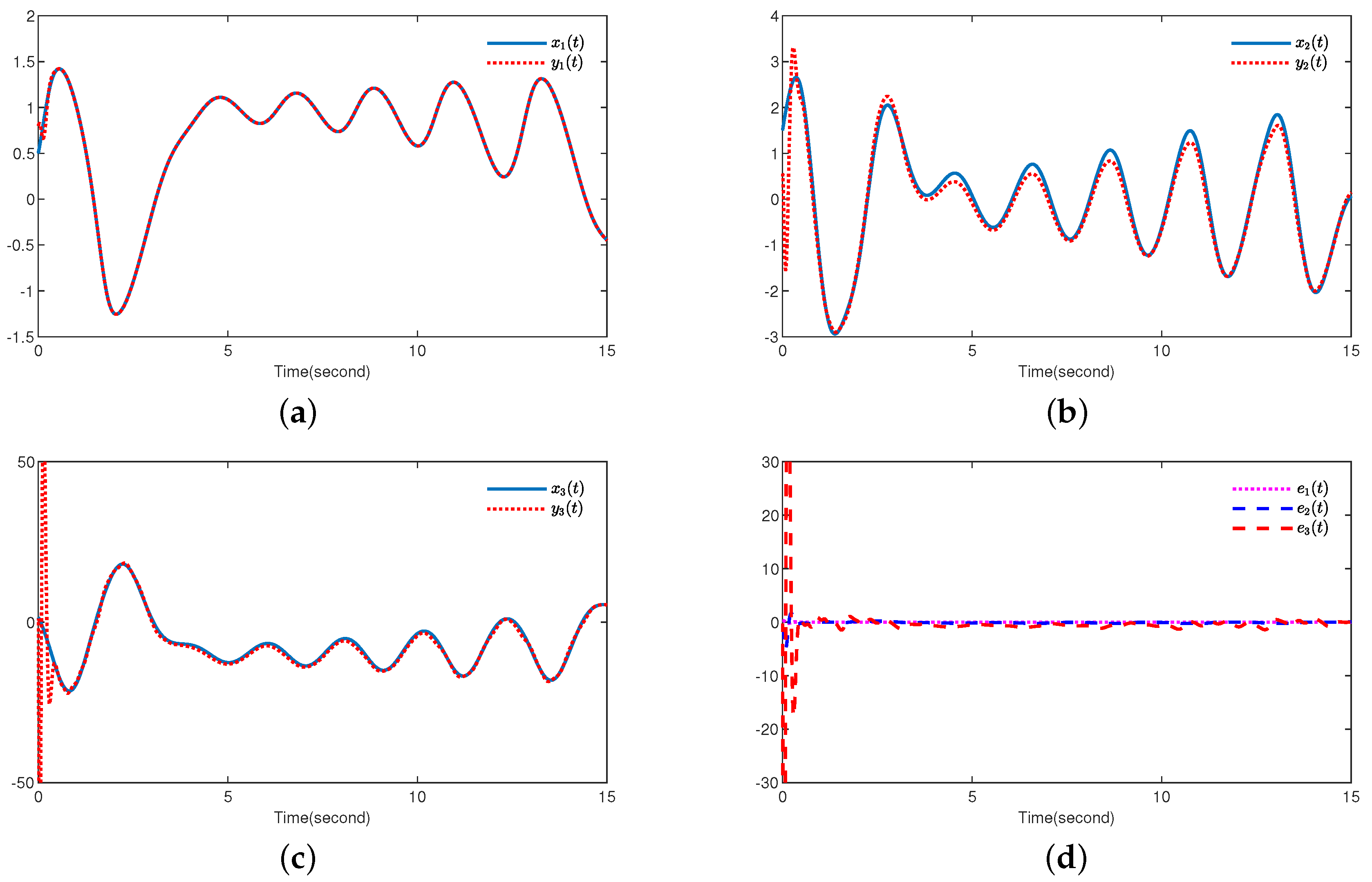
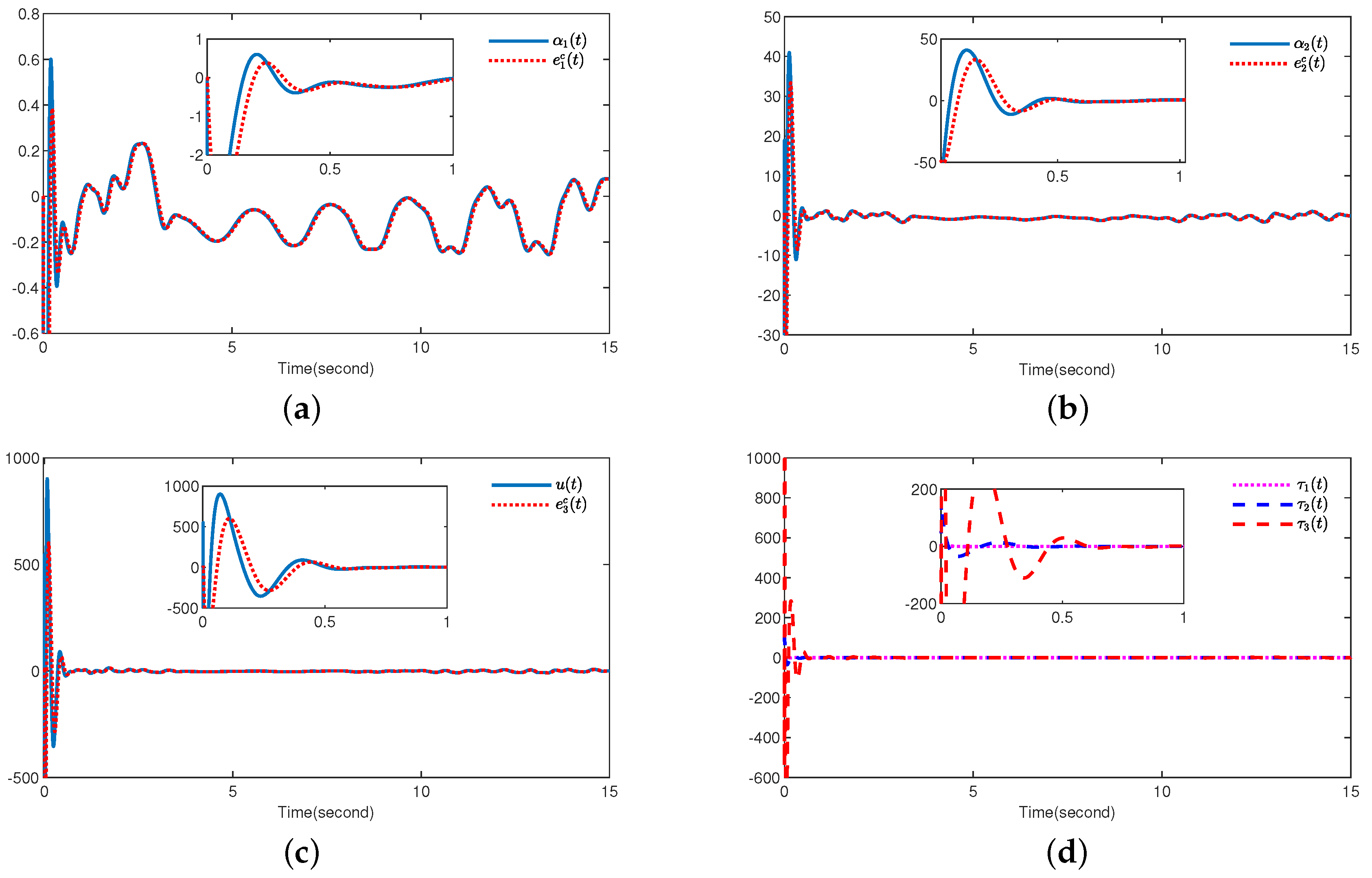
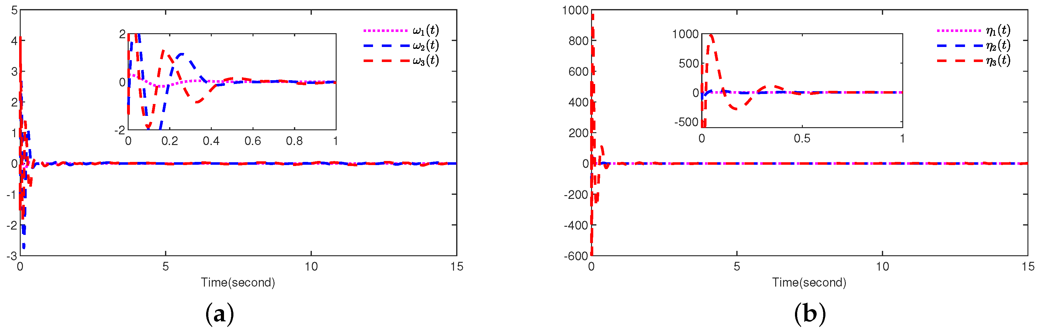
4. Simulation Results

So as to certify the feasibility of the put forward controller for uncertain FOCSs, we premeditate the following systems.

The master system [32] is

$$\left\{\begin{array}{c}{\mathcal{D}}^{\vartheta }{x}_1=x_2+\frac{10}{7}(x_1-x_1^3),\hfill \\ {\mathcal{D}}^{\vartheta }{x}_2=x_3+10x_1-x_2,\hfill \\ {\mathcal{D}}^{\vartheta }{x}_3=-\frac{100}{7}{x}_2.\hfill \end{array}\right.$$

(63)

The slave system [32] is

$$\left\{\begin{array}{c}{\mathcal{D}}^{\vartheta }{y}_1=y_2+\frac{10}{7}(y_1-y_1^3)+0.15sin{x}_1+0.1sin\left(x_1{x}_2\right),\hfill \\ {\mathcal{D}}^{\vartheta }{y}_2=y_3+10y_1-y_2+0.5sin(x_1^2+x_2^2)+\frac{1}{10+x_1{x}_2{cos}^{2}t},\hfill \\ {\mathcal{D}}^{\vartheta }{y}_3=-\frac{100}{7}{y}_2+u\left(t\right)+1.5sin{x}_2+\frac{0.3sin\left(x_1{x}_2\right)}{x_1^2+x_2^2+x_3^2}.\hfill \end{array}\right.$$

(64)

The initial conditions are given as $x\left(0\right)=[x_1\left(0\right)$, $x_2\left(0\right)$, $x_3\left(0\right){]}^T=[0.5$, $1.5$, ${1.5]}^T$, $y\left(0\right)=[y_1\left(0\right)$, $y_2\left(0\right)$, $y_3\left(0\right){]}^T=[0.8$, $0.5$, ${0.5]}^T$, $e_1^c\left(0\right)=e_2^c\left(0\right)=e_3^c\left(0\right)=0$, ${\alpha }_1\left(0\right)={\alpha }_2\left(0\right)=u\left(0\right)=0$, ${\widehat{e}}_1={\widehat{e}}_2={\widehat{e}}_3=0$, $\widehat{\gamma }=0$, $\widehat{Q}=0$, $d=0$. The opted parameters are revealed as $\vartheta =0.98$, ${\lambda }_1={\lambda }_2={\lambda }_3=28$, ${\theta }_1={\theta }_2={\theta }_3=2$, $k_1=k_2=20$, $k_3=80$, $s_1=s_2=s_3=10$, ${\sigma }_1={\sigma }_2={\sigma }_3=12$, ${\beta }_1={\beta }_2={\beta }_3=0.001$, $m_1=m_2=m_3=9$, ${\delta }_1={\delta }_2={\delta }_3=9.5$.

There are three FLSs adopted in the devised controller. The first FLS takes $x_1$ and $y_1$ as its input and defines nine Gaussian membership functions evenly distributed on $[-2$, $2]$ for every input. The initial condition is picked as ${\rho }_1\left(0\right)=[1$, …, ${1]}^T\in {\mathbb{R}}^{81}$. The second FLS takes $x_1$, $x_2$, $y_1$ and $y_2$ as its input and defines four Gaussian membership functions evenly distributed on $[-3$, $3]$ for every input. The initial condition is picked as ${\rho }_2\left(0\right)=[1$, …, ${1]}^T\in {\mathbb{R}}^{256}$. The third FLS takes $x_3$ and $y_3$ as its input and defines 10 Gaussian membership functions evenly distributed on $[-25$, $20]$ for every input. The initial condition is picked as ${\rho }_3\left(0\right)=[1$, …, ${1]}^T\in {\mathbb{R}}^{100}$.

Ultimately, the simulation outcomes are exhibited in Figure 1, Figure 2, Figure 3, Figure 4 and Figure 5. Figure 1 exhibits that the master–slave systems are practically synchronized and their synchronization errors converges to a small neighborhood of the origin, which shows that the proposed method has excellent control performance. Figure 2 displays the approximation effect of ${\mathsf{\Phi }}_i$, and the simulation results show that the proposed compound AFBC method has obvious improvement effect on FLS. Figure 3 exhibits the approximation effect of the virtual input ${\alpha }_i$ and the actual input u, from which we can find that the filter adopted has a strong approximation effect. The tracking errors by using the compound AFBC and the tracking error compensation signals are exhibited in Figure 4. Figure 5 displays the approximation effect of ${\gamma }_i$, and the simulation results show that the proposed DOB can effectively improve the approximation effect by adding a series parallel model compared with the existing DOB. The above results show that the synchronization error has a fast convergence and the controller is able to work well with external disturbances and model uncertainties. Further, we can also observe that all signals can remain bounded, so the control objective is achieved.

5. Conclusions

In this paper, a compound AFBC scheme is proposed for two FOCSs with strict feedback. At each step, a FLS is utilized to approximate a unknown function, and a command filter is taken to approximate the derivative of the virtual control input. Simultaneously, a DOB is adopted to approximate a unknown disturbance. All signals are shown to be bounded and the synchronization errors asymptotically approached to zero by the advanced adaptive fuzzy backstepping controller. Finally, from the simulation results, it can also be intuitively seen that the proposed scheme achieves satisfactory synchronization. How to devise a compound AFBC scheme for FOCSs with input delay is one of our next research directions.

References

1. Wang, S.; He, S.; Yousefpour, A.; Jahanshahi, H.; Repnik, R.; Perc, M. Chaos and complexity in a fractional-order financial system with time delays. Chaos Solitons Fractals 2020, 131, 109521. [Google Scholar] [CrossRef]
2. Homaeinezhad, M.; Yaqubi, S.; Gholyan, H. Control of MIMO mechanical systems interacting with actuators through viscoelastic linkages. Mech. Mach. Theory 2020, 147, 103763. [Google Scholar] [CrossRef]
3. Cunha-Filho, A.; Briend, Y.; de Lima, A.; Donadon, M. A new and efficient constitutive model based on fractional time derivatives for transient analyses of viscoelastic systems. Mech. Syst. Signal Process. 2021, 146, 107042. [Google Scholar] [CrossRef]
4. He, Y.; Zhang, Y.; Sari, H.M.K.; Wang, Z.; Lü, Z.; Huang, X.; Liu, Z.; Zhang, J.; Li, X. New insight into Li metal protection: Regulating the Li-ion flux via dielectric polarization. Nano Energy 2021, 89, 106334. [Google Scholar] [CrossRef]
5. Bouzeriba, A.; Boulkroune, A.; Bouden, T. Projective synchronization of two different fractional-order chaotic systems via adaptive fuzzy control. Neural Comput. Appl. 2016, 27, 1349–1360. [Google Scholar] [CrossRef]
6. Khan, A.; Jahanzaib, L.S. Synchronization on the adaptive sliding mode controller for fractional order complex chaotic systems with uncertainty and disturbances. Int. J. Dyn. Control 2019, 7, 1419–1433. [Google Scholar] [CrossRef]
7. Wei, Z. Dynamical behaviors of a chaotic system with no equilibria. Phys. Lett. A 2011, 376, 102–108. [Google Scholar] [CrossRef]
8. Qi, G.; Chen, G.; Du, S.; Chen, Z.; Yuan, Z. Analysis of a new chaotic system. Phys. A Stat. Mech. Its Appl. 2005, 352, 295–308. [Google Scholar] [CrossRef]
9. Fradkov, A.L.; Evans, R.J. Control of chaos: Methods and applications in engineering. Annu. Rev. Control 2005, 29, 33–56. [Google Scholar] [CrossRef]
10. Yin, X.; Pan, L.; Cai, S. Robust adaptive fuzzy sliding mode trajectory tracking control for serial robotic manipulators. Robot. Comput. Integr. Manuf. 2021, 72, 101884. [Google Scholar] [CrossRef]
11. Boulkroune, A.; Bouzeriba, A.; Bouden, T.; Azar, A.T. Fuzzy adaptive synchronization of uncertain fractional-order chaotic systems. In Advances in Chaos Theory and Intelligent Control; Springer: Berlin/Heidelberg, Germany, 2016; pp. 681–697. [Google Scholar]
12. Huang, S.; Wang, J.; Xiong, L.; Liu, J.; Li, P.; Wang, Z.; Yao, G. Fixed-Time Backstepping Fractional-Order Sliding Mode Excitation Control for Performance Improvement of Power System. IEEE Trans. Circuits Syst. I Regul. Pap. 2021, 69, 956–969. [Google Scholar] [CrossRef]
13. Ha, S.; Liu, H.; Li, S.; Liu, A. Backstepping-based adaptive fuzzy synchronization control for a class of fractional-order chaotic systems with input saturation. Int. J. Fuzzy Syst. 2019, 21, 1571–1584. [Google Scholar] [CrossRef]
14. Shi, X.; Cheng, Y.; Yin, C.; Dadras, S.; Huang, X. Design of fractional-order backstepping sliding mode control for quadrotor UAV. Asian J. Control 2019, 21, 156–171. [Google Scholar] [CrossRef] [Green Version]
15. Moezi, S.A.; Zakeri, E.; Eghtesad, M. Optimal adaptive interval type-2 fuzzy fractional-order backstepping sliding mode control method for some classes of nonlinear systems. ISA Trans. 2019, 93, 23–39. [Google Scholar] [CrossRef]
16. Ha, S.; Chen, L.; Liu, H.; Zhang, S. Command filtered adaptive fuzzy control of fractional-order nonlinear systems. Eur. J. Control 2022, 63, 48–60. [Google Scholar] [CrossRef]
17. Han, S. Fractional-order command filtered backstepping sliding mode control with fractional-order nonlinear disturbance observer for nonlinear systems. J. Frankl. Inst. 2020, 357, 6760–6776. [Google Scholar] [CrossRef]
18. Xue, G.; Lin, F.; Li, S.; Liu, H. Adaptive fuzzy finite-time backstepping control of fractional-order nonlinear systems with actuator faults via command-filtering and sliding mode technique. Inf. Sci. 2022, 600, 189–208. [Google Scholar] [CrossRef]
19. Liu, H.; Wang, H.; Cao, J.; Alsaedi, A.; Hayat, T. Composite learning adaptive sliding mode control of fractional-order nonlinear systems with actuator faults. J. Frankl. Inst. 2019, 356, 9580–9599. [Google Scholar] [CrossRef]
20. Zhou, Y.; Liu, H.; Cao, J.; Li, S. Composite learning fuzzy synchronization for incommensurate fractional-order chaotic systems with time-varying delays. Int. J. Adapt. Control Signal Process. 2019, 33, 1739–1758. [Google Scholar] [CrossRef]
21. Han, Z.; Li, S.; Liu, H. Composite learning sliding mode synchronization of chaotic fractional-order neural networks. J. Adv. Res. 2020, 25, 87–96. [Google Scholar] [CrossRef]
22. Mofid, O.; Mobayen, S.; Khooban, M.H. Sliding mode disturbance observer control based on adaptive synchronization in a class of fractional-order chaotic systems. Int. J. Adapt. Control Signal Process. 2019, 33, 462–474. [Google Scholar] [CrossRef]
23. Li, Z.; Ma, X.; Li, Y. Nonlinear partially saturated control of a double pendulum offshore crane based on fractional-order disturbance observer. Autom. Constr. 2022, 137, 104212. [Google Scholar] [CrossRef]
24. Guha, D.; Roy, P.K.; Banerjee, S. Adaptive fractional-order sliding-mode disturbance observer-based robust theoretical frequency controller applied to hybrid wind–diesel power system. ISA Trans. 2022; in press. [Google Scholar] [CrossRef]
25. Liu, H.; Pan, Y.; Li, S.; Chen, Y. Adaptive fuzzy backstepping control of fractional-order nonlinear systems. IEEE Trans. Syst. Man Cybern. Syst. 2017, 47, 2209–2217. [Google Scholar] [CrossRef]
26. Abbas, S.; Benchohra, M. Fractional order partial hyperbolic differential equations involving Caputo’s derivative. Stud. Univ. Babes-Bolyai Math 2012, 57, 469–479. [Google Scholar]
27. Shen, J.; Lam, J. Non-existence of finite-time stable equilibria in fractional-order nonlinear systems. Automatica 2014, 50, 547–551. [Google Scholar] [CrossRef]
28. Aguila-Camacho, N.; Duarte-Mermoud, M.A.; Gallegos, J.A. Lyapunov functions for fractional order systems. Commun. Nonlinear Sci. Numer. Simul. 2014, 19, 2951–2957. [Google Scholar] [CrossRef]
29. Li, J.; Cao, J.; Liu, H. State observer-based fuzzy echo state network sliding mode control for uncertain strict-feedback chaotic systems without backstepping. Chaos Solitons Fractals 2022, 162, 112442. [Google Scholar] [CrossRef]
30. Zirkohi, M.M. Robust adaptive backstepping control of uncertain fractional-order nonlinear systems with input time delay. Math. Comput. Simul. 2022, 196, 251–272. [Google Scholar] [CrossRef]
31. Ha, S.; Chen, L.; Liu, H. Command filtered adaptive neural network synchronization control of fractional-order chaotic systems subject to unknown dead zones. J. Frankl. Inst. 2021, 358, 3376–3402. [Google Scholar] [CrossRef]
32. Petráš, I. Fractional-Order Nonlinear Systems: Modeling, Analysis and Simulation; Springer Science & Business Media: Berlin/Heidelberg, Germany, 2011. [Google Scholar]
Figure 1. Synchronization performance: (a) synchronization performance among x 1 and y 1 ; (b) synchronization performance among x 2 and y 2 ; (c) synchronization performance among x 3 and y 3 ; (d) synchronization errors.
Fractalfract 06 00652 g001
Figure 2. Comparison results: (a) the approximation effect of Φ 1 by utilizing the compound AFBC; (b) the approximation effect of Φ 1 by utilizing the AFBC; (c) the approximation effect of Φ 2 by utilizing the compound AFBC; (d) the approximation effect of Φ 2 by utilizing the AFBC; (e) the approximation effect of Φ 3 by utilizing the compound AFBC; (f) the approximation effect of Φ 3 by utilizing the AFBC.
Fractalfract 06 00652 g002
Figure 3. Time response of filters: (a) virtual input α 1 and filter output e 1 c ; (b) virtual input α 2 and filter output e 2 c ; (c) actual input u and filter output e 3 c ; (d) filter errors.
Fractalfract 06 00652 g003
Figure 4. Auxiliary variables: (a) tracking errors by using the compound AFBC; (b) tracking error compensation signals.
Fractalfract 06 00652 g004
Figure 5. Comparison results: (a) the approximation effect of γ 1 by utilizing the compound AFBC; (b) the approximation effect of γ 1 by utilizing the AFBC; (c) the approximation effect of γ 2 by utilizing the compound AFBC; (d) the approximation effect of γ 2 by utilizing the AFBC; (e) the approximation effect of γ 3 by utilizing the compound AFBC; (f) the approximation effect of γ 3 by utilizing the AFBC.
Fractalfract 06 00652 g005
Publisher’s Note: MDPI stays neutral with regard to jurisdictional claims in published maps and institutional affiliations.