Analysis of 2D and 3D Convolution Models for Volumetric Segmentation of the Human Hippocampus

Abstract

Extensive medical research has revealed evidence of a strong association between hippocampus atrophy and age-related diseases such as Alzheimer’s disease (AD). Therefore; segmentation of the hippocampus is an important task that can help clinicians and researchers in diagnosing cognitive impairment and uncovering the mechanisms behind hippocampal changes and diseases of the brain. The main aim of this paper was to provide a fair comparison of 2D and 3D convolution-based architectures for the specific task of hippocampus segmentation from brain MRI volumes to determine whether 3D convolution models truly perform better in hippocampus segmentation and also to assess any additional costs in terms of time and computational resources. Our optimized model, which used 50 epochs and a mini-batch size of 2, achieved the best validation loss and Dice Similarity Score (DSC) of 0.0129 and 0.8541, respectively, across all experiment runs. Based on the model comparisons, we concluded that 2D convolution models can surpass their 3D counterparts in terms of both hippocampus segmentation performance and training efficiency. Our automatic hippocampus segmentation demonstrated potential savings of thousands of clinician person-hours spent on manually analyzing and segmenting brain MRI scans

1. Introduction

Magnetic resonance imaging (MRI) is a powerful, non-invasive clinical tool used for numerous purposes in the health industry that range from diagnosing patients to the study of diseases. MRI scanners work by employing strong magnets to produce a magnetic field that aligns the protons in the body, causing them to release energy that is picked up by sensors [1]. As different tissues in the body have varying elemental compositions, each of them tends to release different amounts of energy. Further processing and transformation of these energy signals then produces the final magnetic resonance (MR) images.

With rapid advances in MRI technology throughout the past decades, researchers have been able to study structures of the brain in increasing detail. Unlike some medical imaging techniques such as X-rays that generate two-dimensional images, MRI machines output three-dimensional volumes, allowing clinicians to better visualize the spatial relationship between brain structures. While there are many variations of MRI modes, this paper will focus on T1-weighted (T1W) MRI because it is especially suitable for identifying structures in the brain [2]. Further improvements in MRI technology have allowed researchers to better gather quantitative information such as the concentration of iron in parts of the brain and the volumes of certain brain structures such as the hippocampus [3].

The hippocampi are two complex structures in the left and right human brain that play an important role in memory and cognitive function [4]. Morphology, volume, and other physical characteristics of each hippocampus can be deduced by identifying regions of the brain corresponding to the hippocampus in a process known as hippocampus segmentation. Extensive medical research has also revealed evidence of a strong association between hippocampus atrophy and age-related diseases such as Alzheimer’s disease (AD) [4,5,6]. Therefore, segmentation of the hippocampus is an important task that can help clinicians and researchers in diagnosing cognitive impairment and uncovering the mechanisms behind hippocampal changes and diseases of the brain.

The “gold standard” of hippocampus segmentation is manual segmentation, in which an expert in neuroanatomy will manually trace out the hippocampus from high-resolution magnetic resonance (MR) images. However, this approach is extremely time-consuming and also requires the presence of an expert who is very familiar with studying brain structures from MR images [7]. Furthermore, there may be significant variation between how two different experts identify the hippocampus, leading to considerable inconsistencies between manual segmentations, although there have been recent attempts made toward a standardized manual segmentation protocol [8]. These difficulties faced in manual segmentation has led to the research and development of algorithms for automatic hippocampus segmentation, which can provide fast, consistent results for large datasets of MR images.

Today, most automatic segmentation algorithms make use of different variations of atlas-based techniques [9]. In the context of hippocampus segmentation, an atlas refers to a MR image that contains an ideal segmentation of the hippocampus [10]. An atlas must be transformed to be aligned with a common coordinate system in a process known as registration, which ensures spatial correspondence with other MR images registered to the same system [11]. The atlas images can also be compiled MR images generated from the MR images of multiple individuals from the population. One such example is the MNI ICBM-152 brain volume template prepared by the Montreal Neurological Institute (MNI), McGill University [12]. This brain volume template was generated by averaging over 152 normal brain MR images co-registered onto the same coordinate system.

The simplest atlas-based method is single atlas, which starts off with the input MR image being registered to the atlas image using a series of linear and non-linear transformations. This ensures that the MR image is as similar as possible to the atlas image. The inverse of the transformation used to register the input image is then applied to the hippocampus segmentation of the atlas image, thus generating the segmented hippocampus in the input image [10]. Although this method is simple and relatively quick, its main disadvantage is that the predicted segmentation is heavily dependent on the atlas image used. If the anatomy of the individual differs greatly from that of the atlas, then the predicted segmentation will be inaccurate.

Algorithms using the probabilistic atlas have a much lower computational cost since registration between the atlases is done at the start of the method, and new target MR images do not have to be individually registered to every atlas used. However, decent hippocampus segmentation results are still obtained using this method [10]. Popular brain MRI software such as FreeSurfer and FMRIB Software Library (FSL) use variants of the probabilistic atlas method for their hippocampus segmentation functions [13,14].

Current research on deep learning and hippocampus segmentation are largely focused on the design and creation of architectures that leverage either 2D or 3D convolutions. However, there has been a lack of research to fairly and clearly establish the advantages and disadvantages of using 2D or 3D convolutions for segmenting the hippocampi from volumetric MRI data.

The main aim of this paper was to provide a fair comparison of 2D and 3D convolution-based architectures for the specific task of hippocampus segmentation from brain MRI volumes. It is worth investigating whether 3D convolution models truly perform better in hippocampus segmentation and also to assess any additional costs in terms of time and computational resources. Naturally, one of the main outcomes to track would be how well each model performs for the task of hippocampus segmentation. However, another vital outcome to note is the training speed of each model, which directly affects training efficiency of deep learning models. Deep learning techniques usually require large volumes of data and incur significant costs in terms of computational resources and time. Therefore, training speed is of great relevance when it comes to scenarios such as training on large datasets of MRI volumes or quickly retraining models for use in certain target subpopulations. Throughout this paper, emphasis will not be placed solely on model performance but also on how quickly a well-performing model can be trained.

2. Related Works

Many conventional machine learning methods require extensive data preparation in the form of manual feature engineering in order to obtain suitable representations of the data. These often require a substantial amount of time as well as domain expertise, thus making these methods less suitable for raw, unstructured data such as images. To avoid this issue, a family of techniques known as representation learning are used. These techniques are able to accept raw data, automatically discover suitable representations for the data, and either pass these representations on to another algorithm or use them directly for prediction [15]. Deep learning is a form of representation learning that uses compositions of non-linear transformations to form several levels of representations with each level of representation progressively built up with information from the previous levels. Deep learning is usually conducted using artificial neural networks (ANNs) with multiple hidden layers. A specific type of ANN known as the convolutional neural network (CNN) enjoys immense popularity in the field of computer vision due to its ability to analyze raw images with minimal processing. Examples of these CNNs include the VGG-16 and ResNet-50 models, which have achieved state-of-the-art results in several image-related tasks such as classification and object detection [16,17].

In the fields of neuroimaging and neuroscience, deep learning is increasingly being explored for the analysis of medical images pertaining to the human brain. One such application is the use of deep learning for hippocampus segmentation. Studies have indicated that for medical image segmentation tasks, deep learning models can outperform current existing atlas-based methods in terms of segmentation accuracy and inference time [18,19,20]. Hence, the use of deep learning for hippocampus segmentation is an area that is currently being actively researched.

In the current literature, the majority of deep learning models developed for hippocampus segmentation were based on the original U-Net architecture proposed by Ronneberger, Fischer, and Brox [21]. Considered to be a type of CNN, the U-Net architecture (as shown in Figure 1) is composed of a contracting (also called downsampling or analysis) path and a symmetrical expanding (also called upsampling or synthesis) path. Within the contracting and expanding paths, “blocks” consisting of convolution operations are used to progressively build up feature maps relevant to the segmentation task. In the contracting path, contextual information regarding the structures to be segmented is learned by the model. In the expanding path, the outputs from the contracting path are then progressively upsampled to give them the same resolution as the original inputs. Additionally, high-resolution feature maps from the contracting path are concatenated to the upsampled feature maps in the expanding path to allow the model to better localize the final segmented regions.

In the context of hippocampus segmentation, 3D MRI volumes are fed as input to the deep learning models. Since the U-Net architecture was originally designed for 2D biomedical images, various modifications were necessary to create models capable of accepting 3D brain MRI volumes for the task of hippocampus segmentation. To put it broadly, most deep learning models designed for hippocampus segmentation either use 3D convolutions instead of 2D convolutions or continue using 2D convolutions and process the 3D volume on a 2D slice-by-slice basis.

One of the first deep learning architectures developed for segmentation of 3D volumes was the 3D U-Net proposed by Çiçek et al. [22]. The 3D U-Net model is a direct extension of the original U-Net—the two architectures are largely similar for both the contracting and expanding paths. The main difference in 3D U-Net is that all 2D operations (e.g., 2D convolution) in the architecture were replaced by their corresponding 3D operations (e.g., 3D convolution). This allowed the 3D U-Net to accept 3D volumetric data as input. Another modification was the doubling of output channels before each maximum pooling (MaxPool) operation to avoid computational bottlenecks, which was recommended by previous studies [23]. The last modification was the addition of batch normalization operations before each activation function. It should be noted that the last two modifications were mainly targeted at reducing computational costs and speeding up the training process [22].

Further building upon the 3D U-Net architecture, Lin et al. [24] proposed a modified architecture known as multi-scale multi-attention U-Net (MSMA U-Net). One of the main modifications was the use of multiple 3D convolution filters of different dimensions instead of just a single filter. It was argued that this allowed the network to combine feature information from varying scales, which helped it to better segment parts of the hippocampus. Additionally, the authors also used attention modules to further process the feature maps from the contracting path before their concatenation to the expanding path. The motivation behind these attention modules was to allow the model to better locate and focus on features that were more important in a similar manner to how the human visual system is able to selectively focus on certain regions of interest in a visual scene.

Another network architecture that makes use of the 3D U-Net is the Spatial WArping Network for Segmentation (SWANS) as proposed by Dinsdale, Jenkinson, and Namburete [25]. In this architecture, the authors first used a network that combined the 3D U-Net with a spatial transformer network to learn a deformation transformation. This transformation then deformed an initial binary segmentation mask (in the shape of an arbitrary sphere) into the true segmentation mask. The main benefit of using the spatial transformer network was that it allowed for better segmentation of hippocampi that were located in different regions across the MRI volumes, which may occur due to bad registration of the MRI scans.

As mentioned above, 2D convolution models process volumetric MRI data by going through them slice-by-slice. In 3D MRI scans, there are three main orthogonal axes from which slices may be taken as shown in Figure 2. Therefore, most 2D convolution models adopt a multi-view approach in which they combine the outputs of several networks with different views to form a final predicted segmentation of the hippocampi.

One such example is the 2D U-Seg-Net architecture and its ensembles as proposed by Chen et al. [26]. The U-Seg-Net is a slightly simplified version of the original U-Net with some convolution operations removed to reduce the number of model parameters. In order to address the issue of 2D convolution models not being able to capture sufficient spatial information in the third dimension, the authors built multiple U-Seg-Net models with each approaching the MRI volume from a different view. Aside from the three orthogonal views, six other diagonal views of the MRI volumes were also explored. The outputs of all the U-Seg-Net models were then used to predict the final hippocampus segmentation mask by combining them using majority voting, which were the 3ViewVote and 9ViewVote models, with the names indicating how many U-Seg-Net models were used. As an additional investigation, the authors also performed stacking by training a CNN called Ensemble-Net, which further processed the inputs of the U-Seg-Net models to produce the final segmentation predictions. The Ensemble-Net was found to have slightly better segmentation performance than the majority voting ensemble models, although it also required more training time.

Another 2D convolution architecture used for hippocampus segmentation is an Ensemble CNN model proposed by Ataloglou et al. [27]. Similar to the U-Seg-Net case, the authors proposed a multi-view approach with a 2D convolution model responsible for each view, although only the three main orthogonal views were used.

A common argument for the use of 3D convolution models to process volumetric data is that they are able to better learn and extract better features from volumes as compared to the 2D convolution models [28,29,30]. This is due to the use of 3D filters during 3D convolutions, which allow the spatial information in the three-dimensional space around each voxel to be better captured, whereas 2D convolutions can only capture the spatial information in the two-dimensional space around each voxel within a slice. A visualization of this is shown in Figure 3. This means that any spatial information across slices that are relevant to identifying the hippocampus is lost when using 2D convolutions from a single view because each slice is processed independently of the others.

However, one counterargument against 3D convolution models is that they are significantly more complex than 2D convolution models and have a large number of parameters within the model to update during training [26,27]. With their large number of parameters, 3D convolution models may have a tendency to overfit (especially when there is insufficient data), thus resulting in a worse segmentation performance on unseen MRI volumes. The large number of parameters also means that significantly more computation time is required to train 3D convolution models as compared to their 2D counterparts. Another vital outcome to note when comparing models is the training speed of each model, which directly affects training efficiency of deep learning models [31]. In this paper, a comparison was made between the 3D U-Net and 2D U-Seg-Net architectures. These two architectures were chosen mainly because of their architectural similarities with each other; the main difference was whether 2D or 3D convolutions were used. No extensive modifications such as the addition of extra network modules (e.g., spatial transformer modules) or training algorithms that further processed the U-Net outputs were used. This helped to ensure that any observed differences in our experimental results could be largely attributed to the type of convolution used in each of these models.

3. Methodology

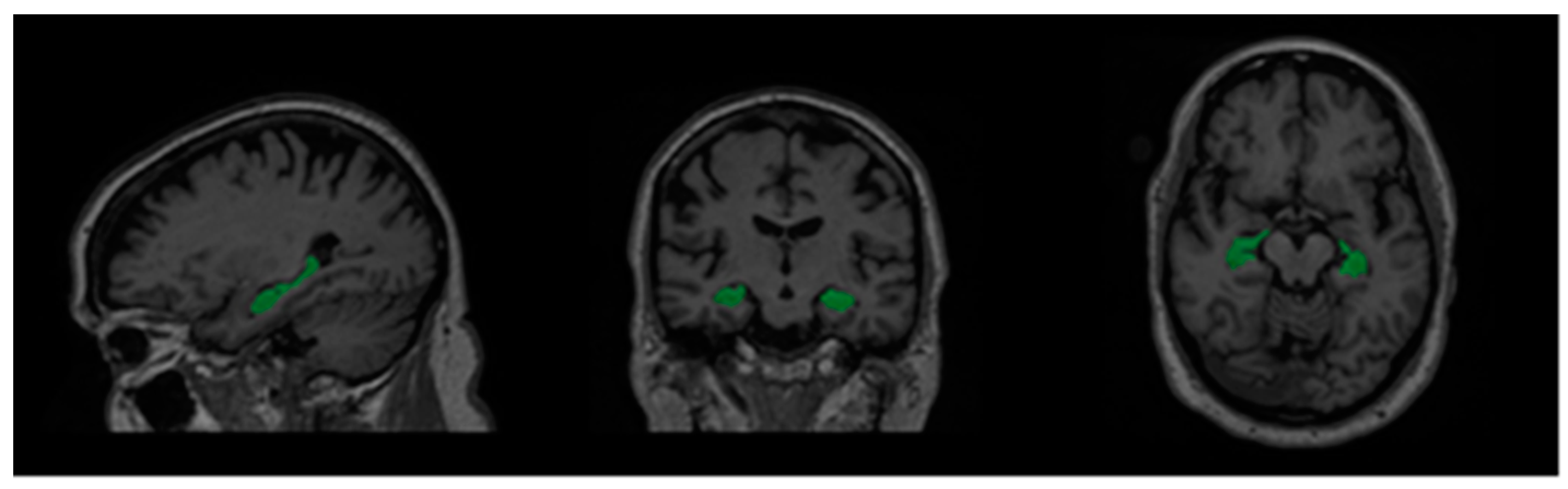
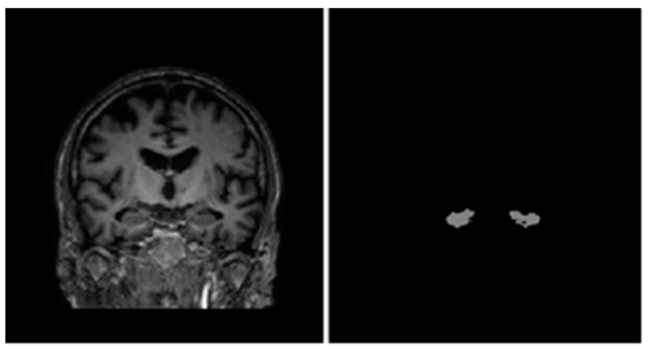
3.1. Data Description

In the context of this paper, it was necessary for our chosen experimental dataset to meet the following criteria:

• Have high-quality hippocampus segmentation masks (preferably from manual segmentation), which have been proven to closely follow the morphometric characteristics of the actual hippocampi;
• Have hippocampus segmentation masks that are obtained using a clinically validated and standardized set of rules in order to ensure their inter-rater reliability;
• Contain sufficient data for both training and evaluation of our models.

Data used in the preparation of this article were obtained from the Alzheimer’s Disease Neuroimaging Initiative (ADNI) database (adni.loni.usc.edu, accessed on 19 March 2022). The ADNI was launched in 2003 as a public–private partnership led by Principal Investigator Michael W. Weiner, MD. The primary goal of ADNI has been to test whether serial magnetic resonance imaging (MRI), positron emission tomography (PET), other biological markers, and clinical and neuropsychological assessment can be combined to measure the progression of mild cognitive impairment (MCI) and early Alzheimer’s disease (AD).

In 2013, a joint project between the European Alzheimer’s Disease Consortium (EADC) and Alzheimer’s Disease Neuroimaging Initiative (ADNI) came up with a standardized protocol for manual segmentation of the hippocampus from MRI scans known as the EADC-ADNI Harmonized Protocol (HarP) [32]. Further follow-up studies showed a significant increase in inter-rater intraclass correlation coefficient (ICC) when experts performing manual segmentations switched to using HarP [8,33]. HarP was also pathologically validated by comparison of HarP segmentations and post-mortem MRI scans of AD patients [34]. Upon establishing the validity of the HarP segmentation method, the EADC-ADNI team also recognized that many automated segmentation algorithms required a large sample of brain MRI volumes and their corresponding hippocampus segmentation masks (segmented with HarP) for training. Therefore, a dataset consisting of 135 brain MRI volumes complete with the benchmark HarP-segmented hippocampus masks was created for use in further research [35]. More information regarding the EADC-ADNI HarP data (including steps to download them) can be found in [36]. It should be noted that for every brain MRI volume, there were two hippocampus segmentation masks corresponding to the left and right hippocampus. A sample coronal view of a brain MRI volume and its corresponding combined hippocampus masks can be seen in Figure 4.

Each brain MRI volume was a cuboid with dimensions of 197 × 233 × 189; each voxel contained a real number representing the intensity of that voxel in the MRI scan. Note that unlike colored images with three RGB channels, each volume only had one channel because MRI scans produce grayscale images.

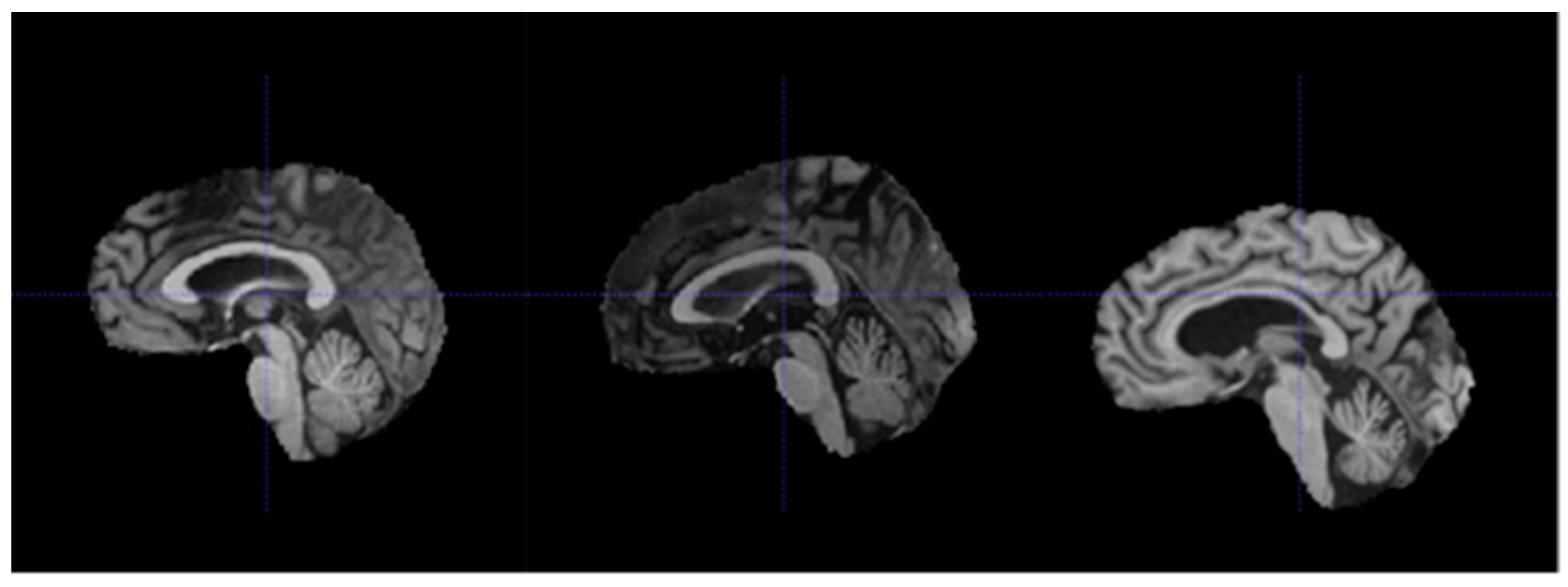
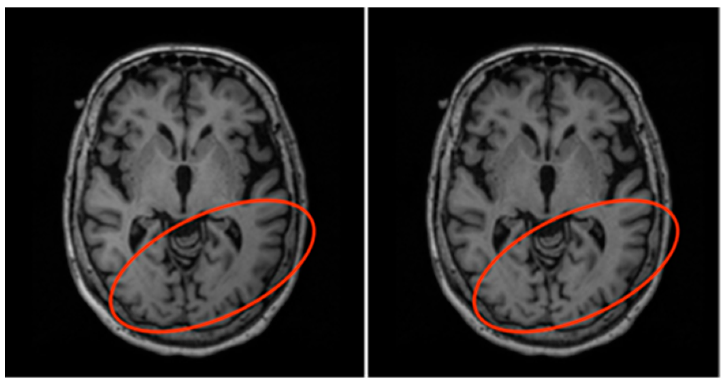
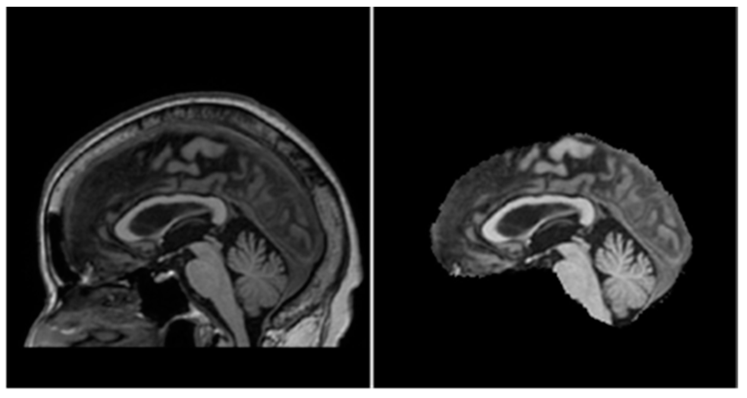
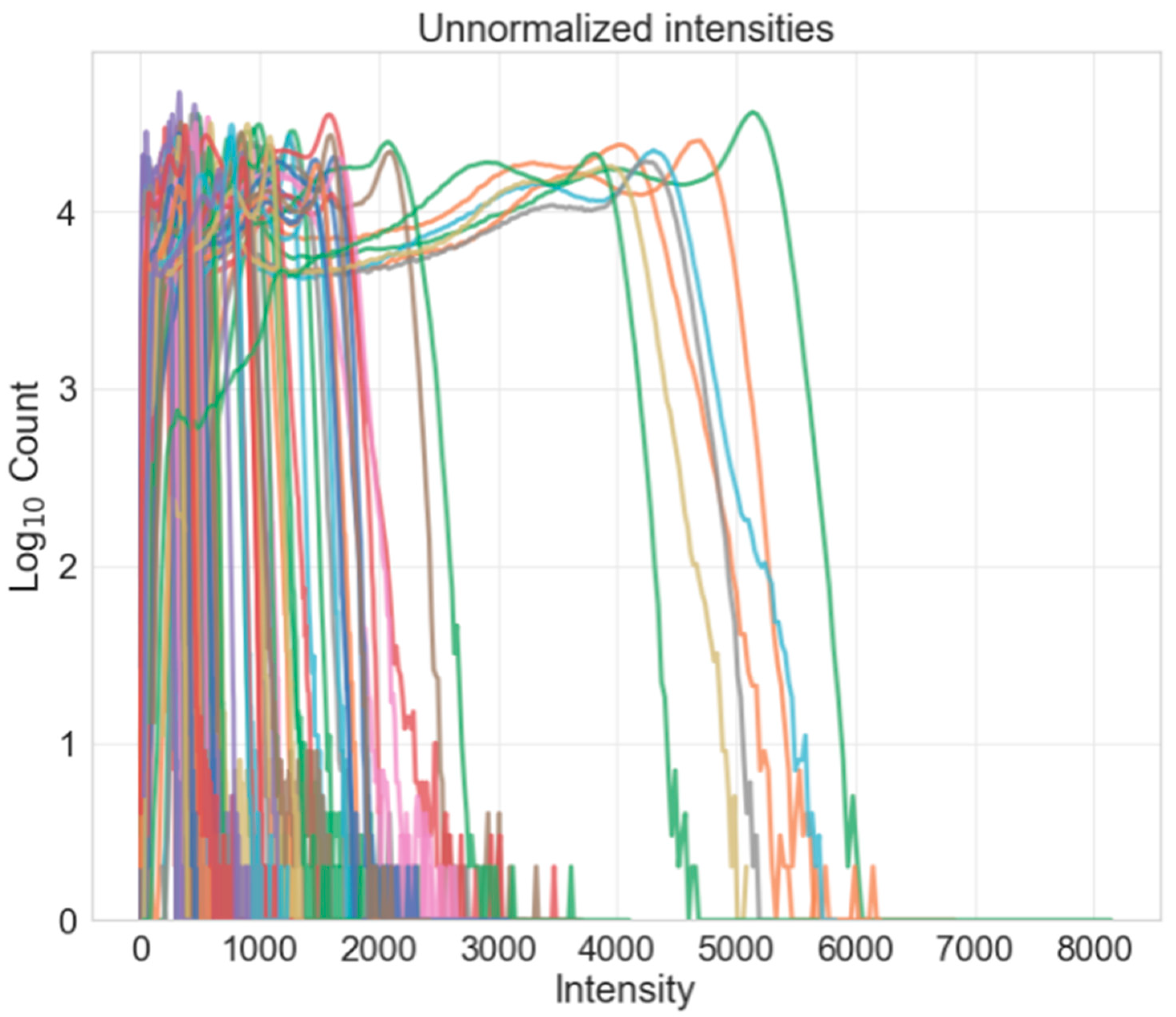
3.2. Data Preparation

Due to the unique nature of MRI data, it was necessary to perform a specific set of pre-processing steps before using the data for training and evaluation. Various studies [37,38,39] have suggested the following steps along with the rationale behind each of them:

• Re-orientation and registration: achieves good alignment of all MRI volumes.
• Field inhomogeneity correction: corrects abnormally dark or bright regions in the MRI volumes caused by inconsistencies in the magnetic field of the scanner.
• Non-brain tissue removal: removes irrelevant tissues such as that of the skull, eyes, and nose, leaving only the brain tissues in each volume.
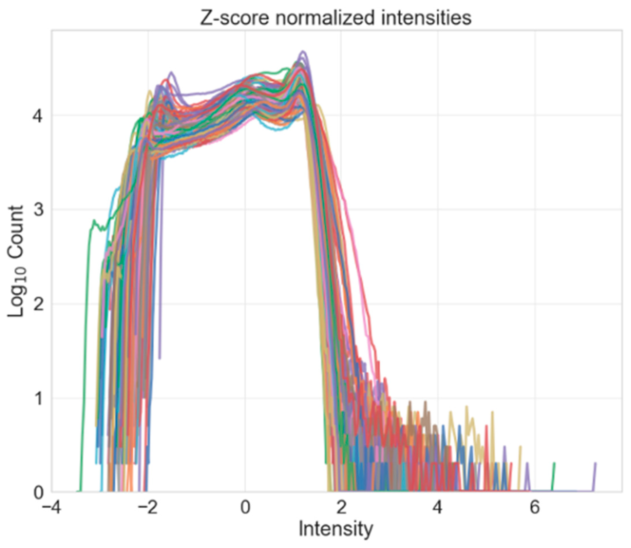
• Intensity normalization: standardizes the intensities of each volume such that the same tissue types in each volume should have the same range of intensity values.

It should be noted that each of the above pre-processing steps was done on a per-subject basis. Therefore, performing these steps prior to splitting the data into training and test sets would not introduce any data leakage. The HarP dataset study indicated that the MRI volumes were already reoriented and registered to the MNI ICBM-152 template with each voxel representing dimensions of 1 × 1 × 1 mm before the HarP segmentations were performed on them. This meant that all 135 MRI volumes should be well aligned and have the same orientation. Further exploration of the data confirmed that all 130 remaining MRI volumes and masks (after removal of anomalous subjects) had the same orientation. However, further examination of the affine transformation matrices associated with each volume suggested the presence of some anomalies.

Generally speaking, each affine transformation matrix (and its inverse) represents the series of transformations required to map each voxel in the volume to a standardized reference space within the scanner [40]. In the HarP dataset, there were 15 subjects with different affine transformation matrices from the rest. One possible explanation is that for these 15 subjects, their MRI scans were taken using a tilted scan angle to obtain oblique scans [37]. Oblique scans are usually used to reduce noise caused by artifacts in the path of the magnetic field, such as air and water within the head of each subject. The use of oblique scans in these 15 subjects meant that even though registration was performed for these subjects, their MRI volumes may still not be as well aligned as those of the other 115 subjects [37]. This was further supported by our observations shown in Figure 5, in which the brain was situated lower in a MRI volume associated with a different affine transformation matrix.

In order to ensure that majority of the brain MRI volumes were well aligned and properly registered, these 15 subjects and their volumes were removed from the dataset. Therefore, the final data consists of the MRI volumes and hippocampus masks of 115 subjects. The next step of pre-processing performed was field inhomogeneity correction, also known as bias field correction. During the acquisition of an MRI scan, the magnetic field weakens as it encounters brain tissue, thereby causing inconsistencies in the intensities through the volumes (even for the same tissue types) [37]. These inconsistencies can make it difficult for the models to accurately detect the boundaries of different tissue types. Therefore, the N4ITK algorithm was used to perform field inhomogeneity correction for all volumes in the dataset [41] as shown in Figure 6 below.

Removal of irrelevant tissues such as those of the eyes, nose, and mouth from brain MRIs, also known as skull-stripping, is essential in reducing the amount of noise within each MRI volume. Iglesias et al. [42] proposed an automated skull-stripping algorithm known as ROBEX that was shown to produce reliable segmentations of the tissues belonging to the brain. With the ROBEX algorithm, all MRI scans in the dataset were skull-stripped to obtain volumes containing just the brain tissues; an example is shown in Figure 7.

Due to differences in the types of scanner used and the configuration of each MRI scan, volumetric MRI data can have very different ranges of intensity values. The intensity values of every MRI volume in the HarP dataset is shown in Figure 8: each line represents the intensity value distribution of each MRI volume. Although every MRI volume had a similarly shaped intensity distribution, the ranges of the intensity values differed greatly. Some MRI volumes had maximum intensity values in the 1000s range, while others had maximum intensity values in the region of 6000.

Intensity normalization brings the intensity values of each MRI volume into a similar range. The key benefit of this is that across all the MRI volumes, voxels corresponding to a specific brain tissue type such as white matter now share a similar range of values. This helps the hippocampus segmentation models better detect the boundaries between different tissue types (using the differences in intensities), thus producing better segmentation masks.

For MRI volumes, Z-score normalization has been shown by studies to be a simple and effective method of intensity normalization [38,39]. For each MRI volume in the HarP dataset, Z-score normalization is performed according to:

$$\widehat{I}\left(\mathbf{x}\right)=\frac{I\left(\mathbf{x}\right)-\mu }{\sigma }$$

(1)

$\widehat{I}$(x) represents the intensity value of the Z score normalized voxel at position x, I(x) represents the intensity value of the original unnormalized voxel at position x, and µ and σ respectively represent the mean and standard deviation of all brain tissue voxel intensities in a subject.

Figure 9 shows the intensity value distribution of each MRI volume after Z-score normalization. It can be seen that the range and distribution of intensity values in all the MRI volumes were much more similar and centered around 0.

In the development of HarP, it was noted that majority of the features useful in identifying a hippocampus were located in and around the hippocampus itself [32]. This meant that a significant portion of each MRI volume did not contain relevant information that could help with the segmentation of the hippocampus. Therefore, for each hippocampus of every subject, a region containing the hippocampus with dimensions of 40 × 56 × 72 was cropped from each brain volume. This cropping was also performed for the segmentation masks. This helped to significantly reduce the computational time and memory requirements of training the model. At the end of all the pre-processing steps, each of the 115 study subjects left in the dataset had two cropped brain volumes corresponding to the regions of interest around the left and right hippocampus as well as two cropped segmentation masks for the left and right hippocampus.

Imbalanced training data may result in the models being biased toward a particular diagnosis stage of AD, while imbalanced test data may lead to an overestimation or underestimation of model performance. Therefore, the data split was performed in a way that ensured the proportion of CN, MCI, and AD subjects were as balanced as possible in both training and test data (see

Table 1. Number of CN, MCI, and AD subjects in training and test data (proportion shown in brackets).

Dataset (n = 115)	CN Subjects	MCI Subjects	AD Subjects
Training (n = 90)	29 (32.2%)	30 (33.3%)	31 (34.4%)
Test (n = 25)	8 (32%)	8 (32%)	9 (36%)

).

Data augmentation is an important component of the deep learning training pipeline (especially when faced with limited training data) because it helps to increase the diversity of training samples and reduces overfitting [43]. In the 3D convolution-based deep learning models designed for hippocampus segmentation, limited training samples is a recurring issue because each model takes in a 3D volume corresponding to one subject as input. For 2D models, this problem is mitigated by the fact that they are restricted to accepting 2D slices as inputs. This means that each MRI volume can provide several training samples for them instead of just one, thus significantly increasing the number of training samples they have and reducing overfitting [26]. For the chosen 3D model, data augmentation was performed on the fly during training. While data augmentation can be performed by generating new MRI volumes and adding them to the dataset, such a method consumes a great deal of memory. Instead, on-the-fly data augmentation randomly applies the augmentation transformation to selected MRI volumes right before they are passed to the model for training without storing them permanently. This achieves the benefits of data augmentation without incurring high memory consumption.

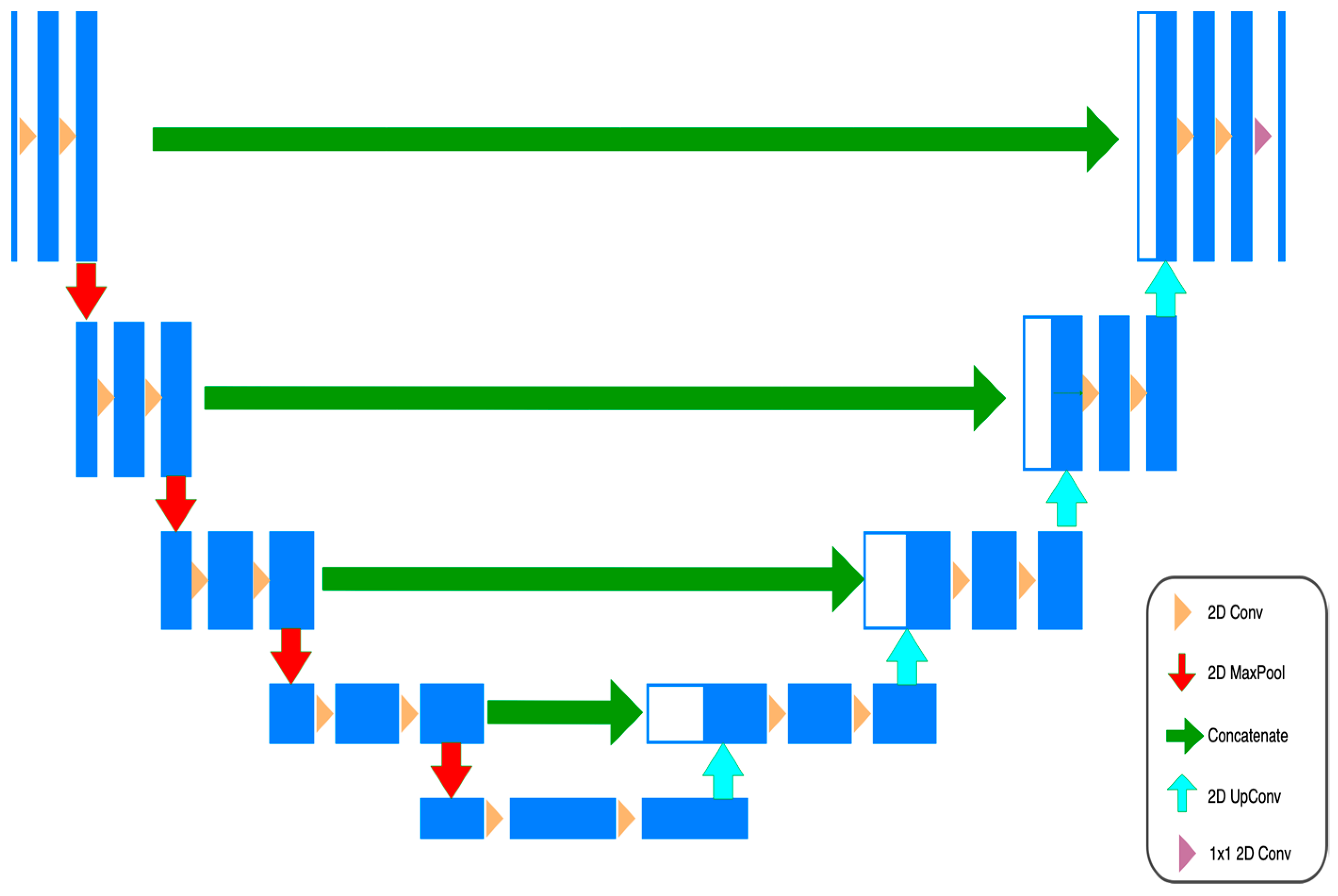
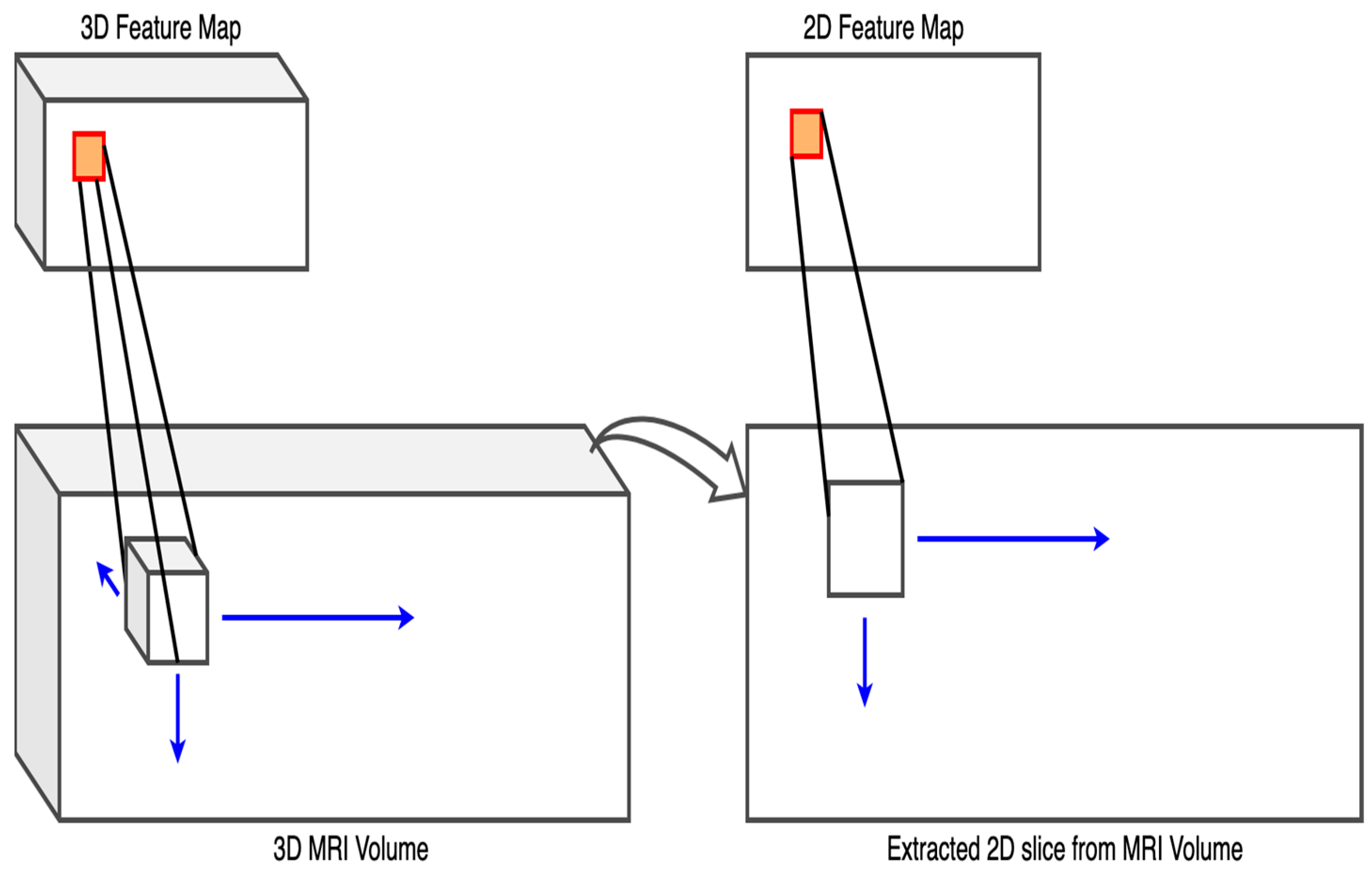
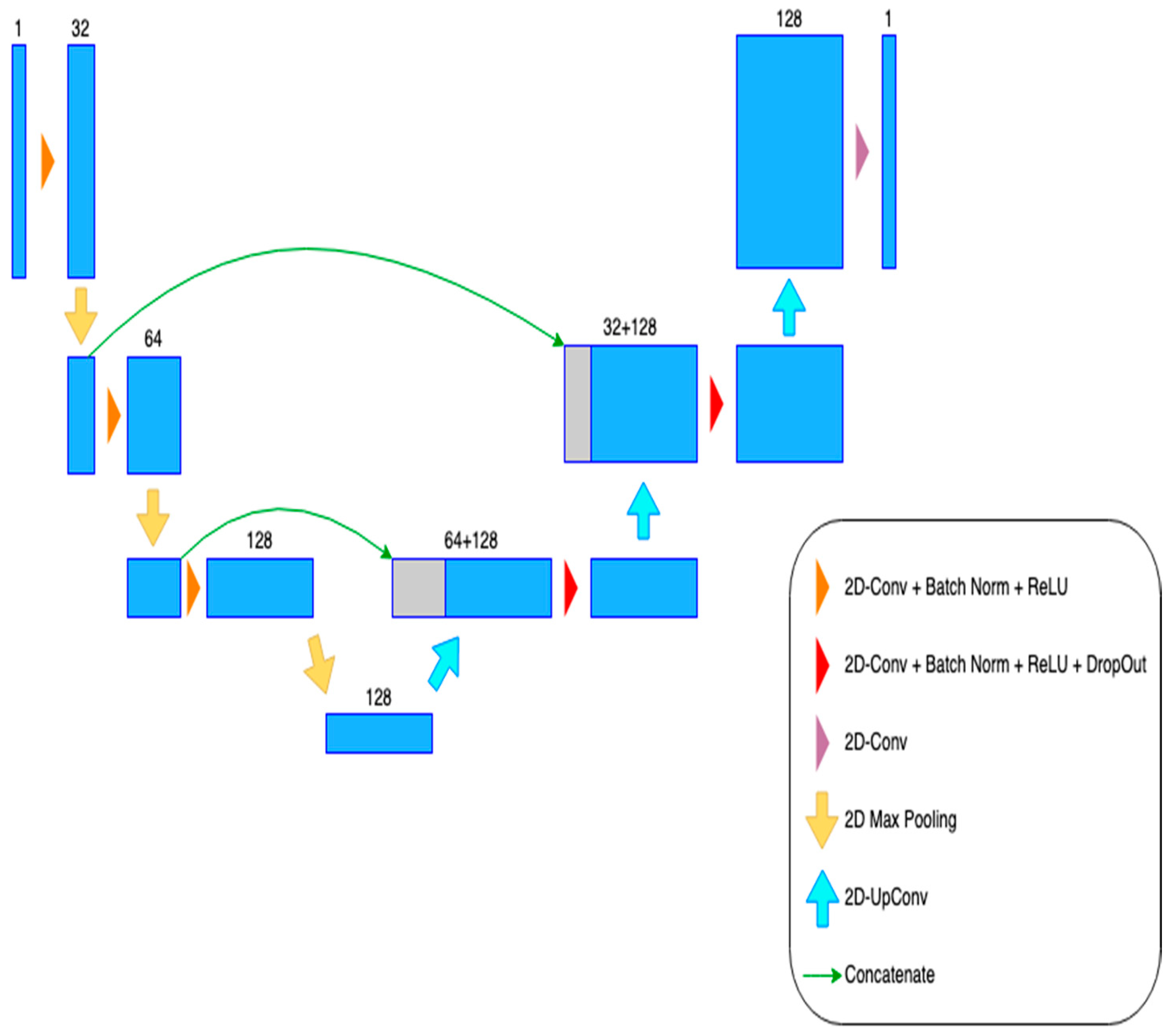
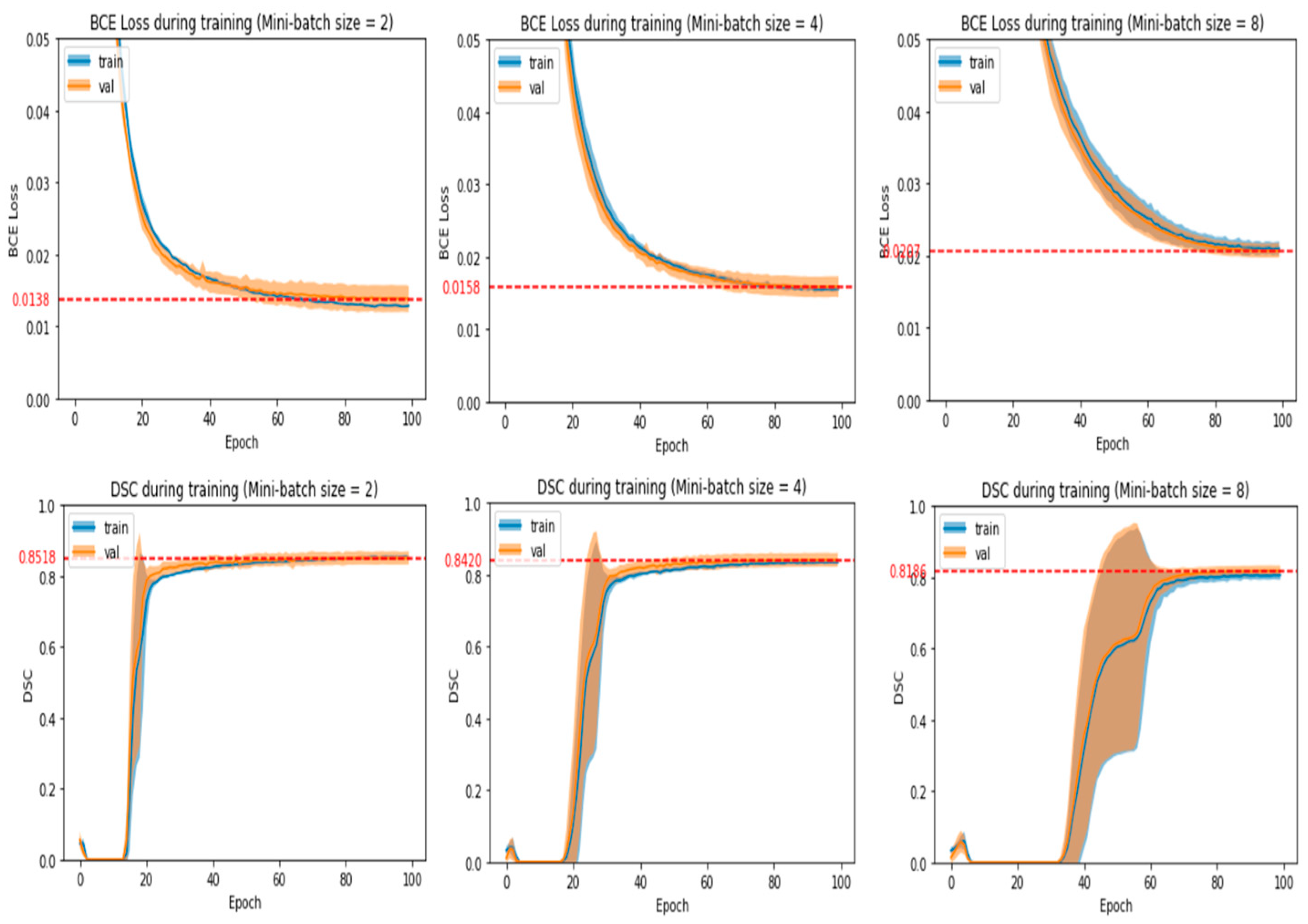
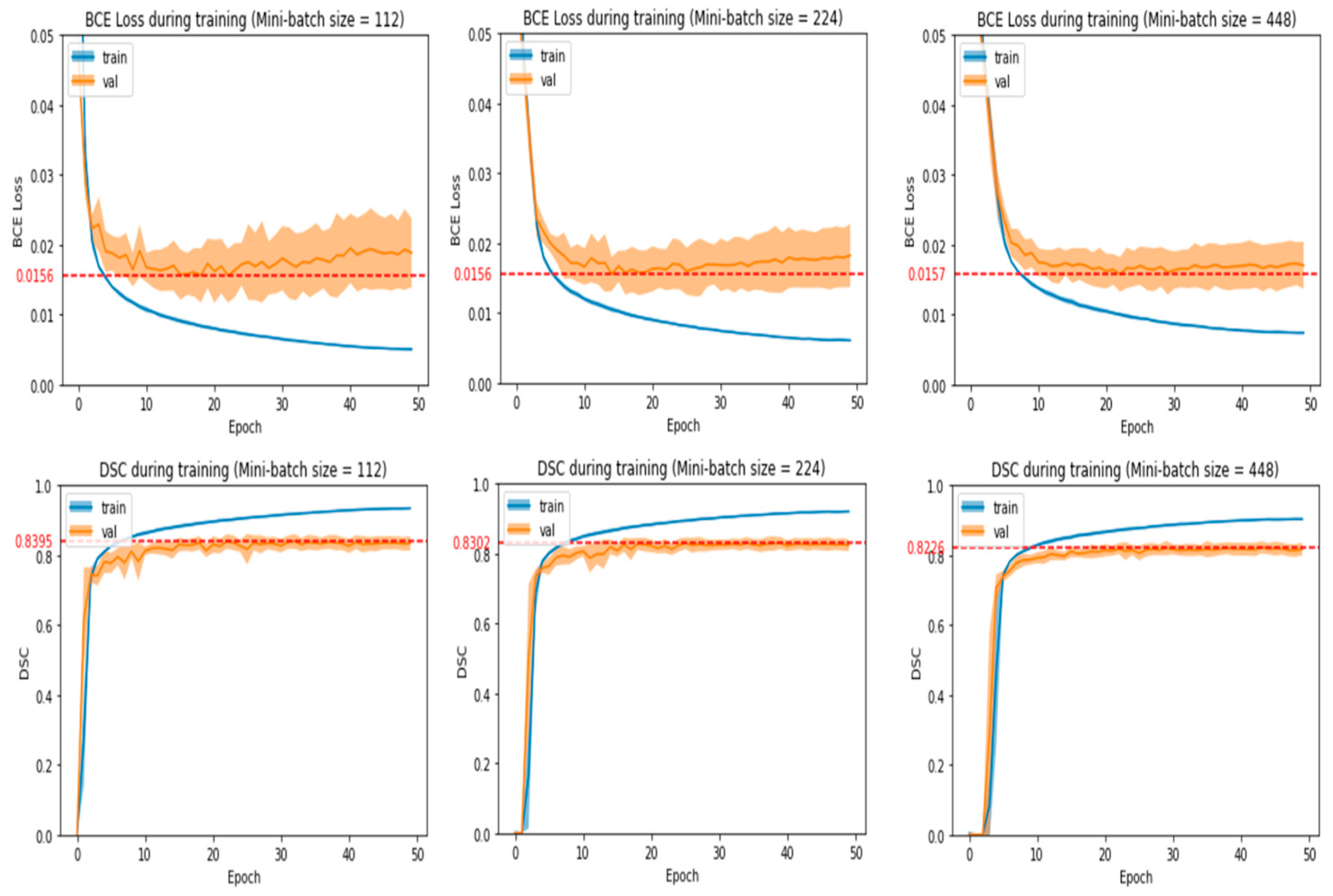
3.3. Training and Model Building

Like most deep learning models, the computed loss and its derivatives are then used to update the model parameters through backpropagation [44]. For the chosen Ensemble U-Seg-Net model, it is important to note that it is not strictly an ANN by itself. Instead, it serves as an aggregation function of the outputs of three 2D U-Seg-Net models, each corresponding to an orthogonal view of an input MRI volume. Therefore, it is important to understand the architecture of the 2D U-Seg-Net model and its differences from the 3D U-Net model.

In Figure 10 below, each rectangle represents a collection of feature maps, and the number above the rectangle represents the number of feature maps. The architecture of each 2D U-Seg-Net is largely based on the original U-Net, slight modifications were made to simplify and optimize the architecture. As shown in Figure 10 the 2D U-Seg-Net contains a contracting path made up of three convolutional blocks followed by an expanding path made up of three deconvolutional blocks. This is largely similar to the 3D U-Net.

Within each convolutional block, a 2D convolution using 3 × 3 filters (each with stride length of 1 in each dimension) was performed once followed by a batch normalization operation and a ReLU activation function. The reason for performing these operations once and not twice as in the 3D U-Net was to reduce the number of parameters in the model, thereby reducing the number of computations required [26]. At the end of each convolutional block, a 2D max-pooling operation with 2 × 2 filters and stride lengths of 2 was applied, thus reducing the resolution of each feature map by half. Similar to the case of 3D U-Net, each convolutional block produced twice the number of feature maps it originally received as input (with the exception of the first block).

The output feature maps of the final convolutional block were then passed directly to the first deconvolutional block in the expanding path. This differed from the 3D U-Net, where further convolutions were performed in the consolidation block before passing the feature maps to the expanding path. Within each deconvolutional block, a 2D transposed convolution operation with 2 × 2 filters and stride lengths of 2 was first applied to the incoming feature maps. The resulting feature maps were then concatenated with feature maps from convolutional blocks in the contracting path with the same resolution. The concatenation of the feature maps in the 2D U-Seg-Net differed slightly from that of the 3D U-Net. Firstly, the feature maps to be concatenated were taken from the convolutional blocks before any convolution was applied (i.e., the start of each convolutional block). Second, there were only two concatenation operations, and no feature maps from the contracting path were concatenated to the last deconvolutional block. These modifications helped to reduce the number of feature maps to be processed in the expanding path, thus further reducing the computational costs. The final step in each deconvolutional block (except for the last one) was then to apply a 2D convolution with 3 × 3 filters (with stride lengths of 1) followed by a batch normalization and the ReLU activation. In addition, dropout operations were added for regularization purposes. After the 2D transposed convolution operation was performed, a simple 2D convolution with a single 3 × 3 filter followed by the sigmoid function was applied to produce an output slice with a single channel.

There was a total of three 2D U-Seg-Net models to be trained; each corresponded to the sagittal, coronal, and axial view slices, respectively. The total number of parameters in each 2D U-Seg-Net model was 697281.

Due to the fact that each U-Seg-Net model took in 2D slices from each subject’s volume, the number of training samples for each model was significantly higher than that of the 3D U-Net. Therefore, as suggested in [26], explicit data augmentation was not performed during the training of each 2D U-Seg-Net model. Instead, the task of regularization to prevent overfitting was performed with the added dropout operations in the U-Seg-Net architecture. The authors of [26] also argued that due to the large number of parameters in 3D convolution models and the limited training samples (since 3D models can only accept 3D volumetric data as input), 3D convolution models were more prone to overfitting. To investigate this, the 3D U-Net and the Ensemble U-Seg-Net models were evaluated on the test data. As a measure of their segmentation performance, the Dice Similarity Coefficient (DSC) was computed for each model as stated in Equation (2) below:

$$\mathrm{DSC}=\frac{2\mathrm{TP}}{2\mathrm{TP}+\mathrm{FP}+\mathrm{FN}}$$

(2)

where TP represents the number of hippocampus voxels correctly predicted by the model, FP represents the number of non-hippocampus voxels wrongly predicted by the model to be part of the hippocampus, and FN represents the number of hippocampus voxels wrongly predicted by the model to not be part of the hippocampus. DSC takes on values between 0 and 1; a higher score indicates a better degree of overlap between the predicted segmentation and ground truth segmentation. As DSC is not significantly affected by class imbalance, it is one of the most popular metrics used for evaluation of image segmentation algorithms, especially in the field of medical imaging [45,46].

The entire training and evaluation pipeline was implemented in Python 3.9.7 with extensive use of the PyTorch deep learning framework [47]. Due to their large numbers of parameters, the training of deep learning models usually requires significant computational resources such as graphics processing units (GPUs) [48]. Each input to the 3D U-Net was a 40 × 56 × 72 volume with a single channel due to the grayscale nature of MRI data. Each element in the input volume represented the intensity value at the corresponding voxel, which could be any real number. The output of the 3D U-Net was also a 40 × 56 × 72 volume with a single channel. However, each element in the output volume was a value between 0 and 1, which represented the probability of the corresponding voxel being part of the hippocampus.

Throughout the entire training process, the test data were not used in any way to prevent data leakage, which may result in overestimation of model performances. In the context of this paper, training of the models aimed to accomplish two things:

• Obtain models that can generalize well to the unseen test data (i.e., have good hippocampus segmentation performance on unseen MRI volumes).
• Train the models in as short amount of time as possible without sacrificing model performance.

Achieving these two aims would allow for fairer comparison of the models, thus giving the findings greater credibility. Therefore, a significant part of the training process was hyperparameter tuning, which is crucial in most machine learning training pipelines. Proper hyperparameter tuning can significantly reduce training times and simultaneously improve performances of models [49].

In deep learning, there are two main groups of hyperparameters: those related to the model design and those related to the training process [50]. Examples of hyperparameters related to model design include number of hidden layers, dropout rates, and choice of activation functions. As this paper’s goal was to compare the two proposed architectures, hyperparameters pertaining to the designs of the models were not changed to avoid modifying their architectures. Instead, hyperparameters such as the learning rate, mini-batch size, and number of epochs were tuned during the training process.

In the training process, the learning rate decided the size of each step taken during updates of the gradient descent-based optimizers. Too large of a learning rate may result in a model being unable to converge, while one that is extremely small may result in excessively long training times. Therefore, the learning rate is widely recognized by many deep learning researchers to be arguably the most important hyperparameter to tune because it plays a huge role in both the model performance as well as the training time of the model [50,51,52].

For clarity, a single experiment run referred to performing 5-fold cross validation for a particular mini-batch size value. The hyperparameters were then chosen based on the following rules:

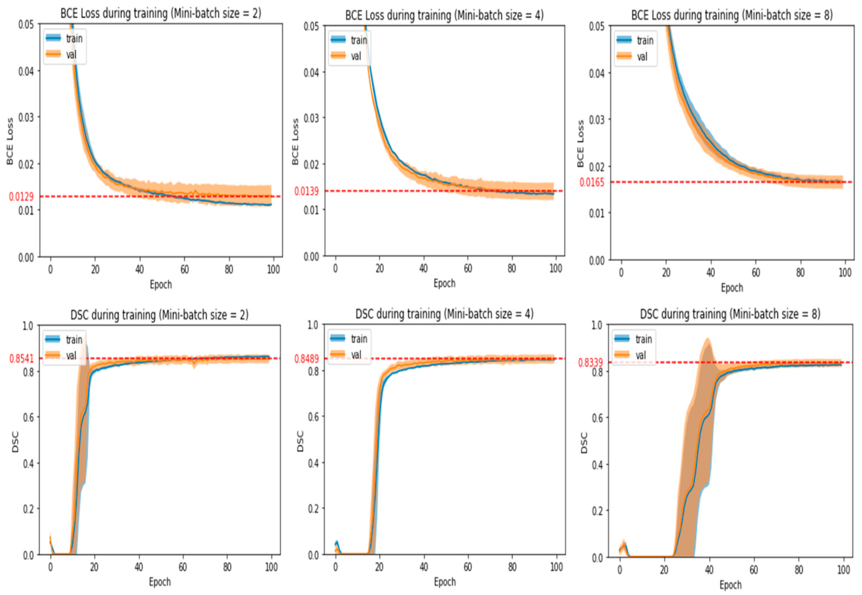
• The number of epochs and mini-batch size chosen should produce average validation loss and DSC that are near the best values obtained in the experiment run.
• Average validation loss and DSC should be stabilized around the chosen number of epochs with no large fluctuations around it. This means that training for a few more or a few less epochs would yield a similar validation loss and DSC.
• If there is an alternative mini-batch size and number of epochs that greatly reduces training time without reducing model performance significantly, then that particular set of hyperparameters will be chosen. After observing some initial experiments, we empirically defined a model’s performance to be significantly affected if the average validation loss increased by more than 0.0004 or the average validation DSC decreased by more than 0.004.

In the above approach, it should be noted that rules 1 and 2 helped in obtaining models with good generalization performance, while rule 3 helped with further optimizing for better training speeds after good generalization performance was achieved.

A slightly modified version of the one-cycle learning rate policy originally proposed by Smith and Topin [53] was adopted for this research. The one-cycle policy is a variant of the cyclical learning rate (CLR) policy proposed in one of Smith’s earlier works, in which he also introduced a method of finding an appropriate upper bound (LRmax) for the learning rate, termed the LR range test [54]. In the CLR policy, learning rates are adjusted in cycles; within each cycle, the learning rate is linearly increased at every update step until LRmax is reached then linearly decreased back down to the initial learning rate in subsequent updates.

According to Smith and Topin [53], using the one-cycle policy has the following advantages:

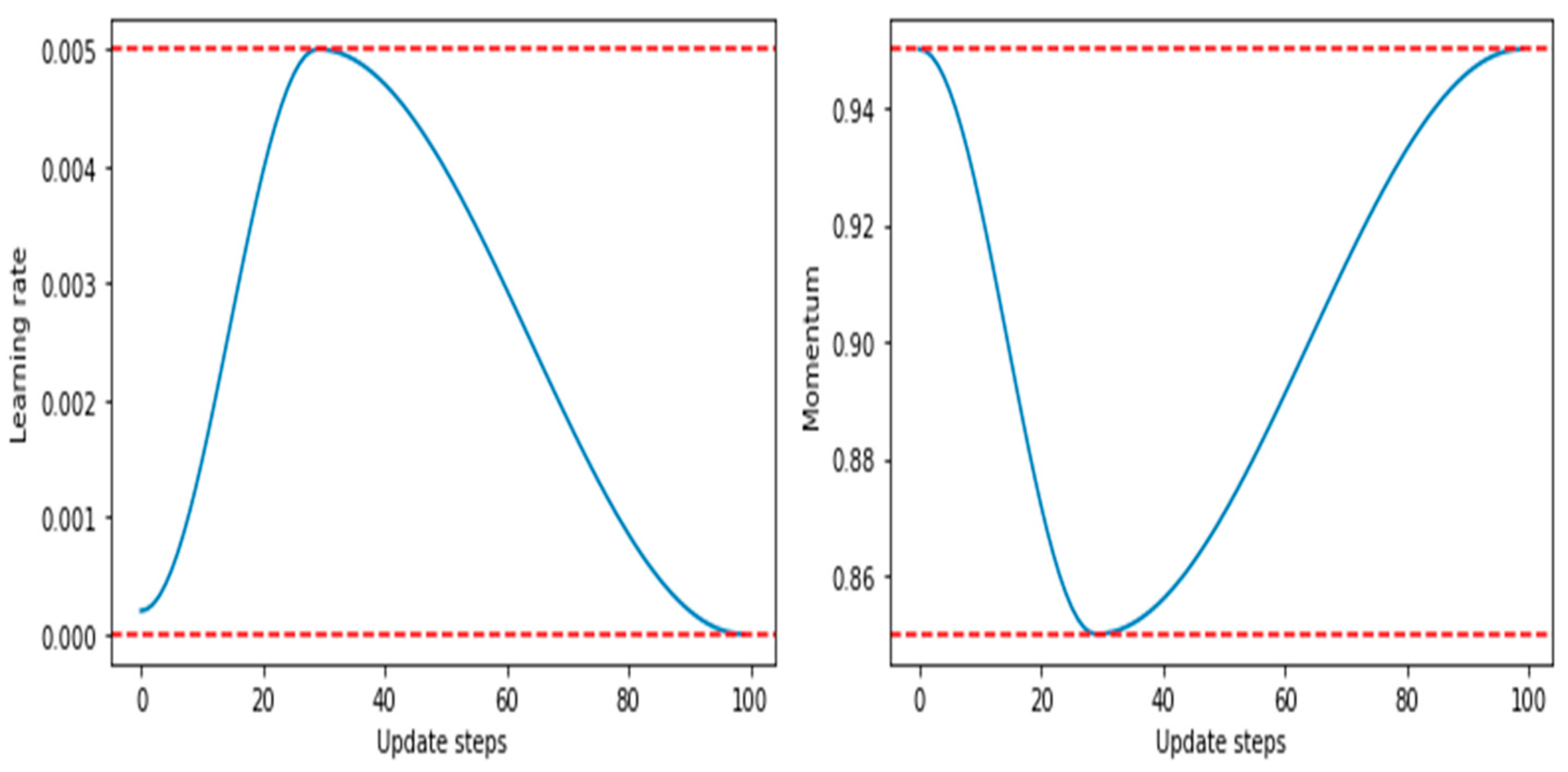
• It achieves a phenomenon termed as super-convergence, in which deep learning models can be trained much faster than with standard training methods.
• It has a proven approach to finding bounds for learning rates (LR range test to find LRmax).
• Its larger learning rates during certain parts of training help to regularize the models, thus reducing the need for other forms of regularization such as weight decay.

In the experiments, this policy was slightly modified such that a cosine annealing schedule was used for increasing the initial learning rate to LRmax (i.e., the first half of the cycle), after which the learning rate was similarly decreased with a cosine annealing schedule from LRmax to zero. Simultaneously, a cosine annealing schedule was also used to decrease momentum from an upper bound of 0.95 to a lower bound of 0.85 in the first half of the cycle then similarly raised back to the upper bound. Figure 11 below shows the simulated adjustments in learning rate and momentum as training progresses. Such an approach has been shown by research to yield better results [55].

Optimization of the model parameters through backpropagation was conducted using a stochastic gradient descent (SGD) optimizer with Nesterov momentum coupled with the modified one-cycle learning rate policy—studies have shown that SGD tends to have better generalization performance compared to other adaptive gradient descent optimizers such as the Adam optimizer [56,57].

Although small mini-batch sizes may result in longer training times (due to more updates per epoch), research has indicated that using large mini-batch sizes for training can hurt the generalization ability of the model [58]. Therefore, mini-batch sizes of 2, 4, and 8 were explored for the 3D U-Net models using a grid-search approach because these values were not too large relative to the training data size.

Determining an appropriate number of epochs to train the models was also a vital step because training for too few epochs could result in the models being unable to learn well, while training for too many epochs could result in the models overfitting to training data. Additionally, the number of epochs was also directly related to how long it took to train the models, which was one of the outcomes of interest. The initial experiments performed indicated that the 3D U-Net models converged well within 100 training epochs, while the U-Seg-Net models generally converged within 50 training epochs. Therefore, epoch numbers in the range of [1, 100] and [1, 50] were explored for 3D U-Net and U-Seg-Net models, respectively.

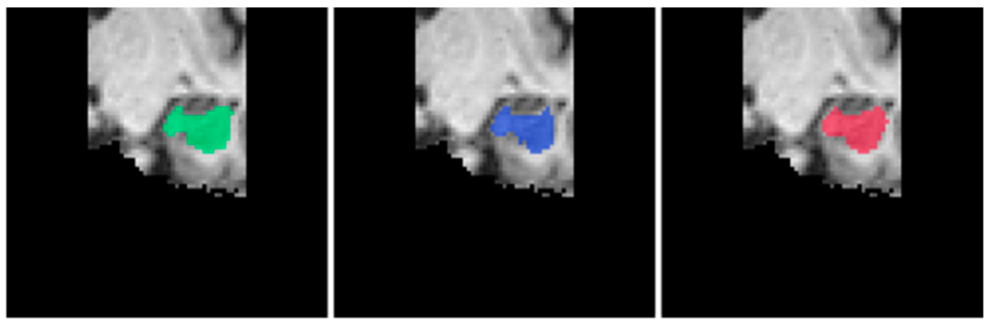
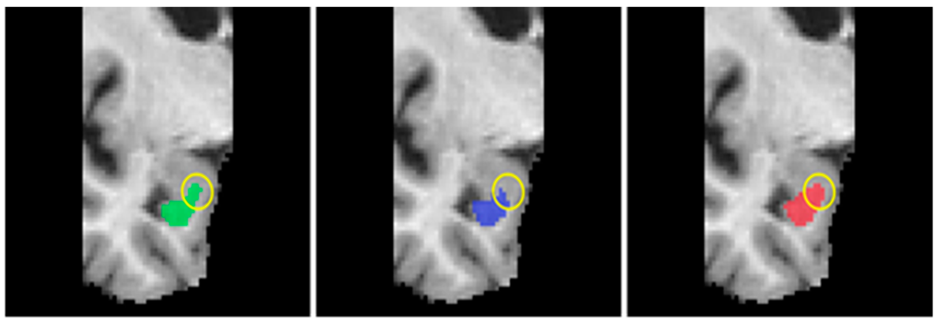
4. Results and Findings

4.1. Segmentation Performance Comparison

With this LRmax, 5-fold cross validation was performed for mini-batch sizes of 2, 4, and 8. The cross-validation results are shown in Figure 12. The average time taken to train one epoch for each of the different mini-batch sizes experimented on are also reported in

Table 2. Training time per epoch for different mini-batch sizes for 3D U-Net_L.

Mini-Batch Size	Training Time per Epoch (s)
2	8.58
4	8.57
8	8.64

.

Based on the validation results, it was observed that using a mini-batch size of 2 achieved the best validation loss and DSC of 0.0129 and 0.8541, respectively, across all experiment runs. Setting the number of training epochs to 50 was also suitable since the validation loss and DSC did not improve much when training for more than 50 epochs.

Another observation was that when larger mini-batches were used, the model converged slower. This meant that the model required more training epochs to reach the optimum validation loss and DSC. Furthermore, Table 2 shows that using larger mini-batches for 3D U-Net_L training did not result in a significant reduction in training time per epoch. Combined with the higher number of training epochs required, this indicated that the larger mini-batches would require a longer training time with no improvement to 3D U-Net_L’s generalization performance.

Therefore, the optimum set of hyperparameters to use for 3D U-Net_L was a mini-batch size of 2 with 50 training epochs.

Similar to the 3D U-Net_L experiments, the LR range test was first performed to find a suitable value of LRmax for the 3D U-Net_R model. Based on the results, the selected LRmax for 3D U-Net_R was 0.0035; the 5-fold cross validation results and training time per epoch are shown below in Figure 13 and

Table 3. Training time per epoch for different mini-batch sizes for 3D U-Net_R.

Mini-Batch Size	Training Time per Epoch (s)
2	8.52
4	8.53
8	8.52

, respectively.

The results of the 5-fold cross validation for 3D U-Net_R were largely similar to that of 3D U-Net_L: the best validation loss (0.0138) and DSC (0.8518) were achieved with a mini-batch size of 2. An appropriate number of epochs to train for was 60 since model performance did not significantly improve beyond 60 epochs. Training with larger mini-batches caused the 3D U-Net_R to converge slower and required more training epochs. Just as in the case of 3D U-Net_L, larger mini-batches did not reduce the training time per epoch significantly.

Therefore, the optimum set of hyperparameters to use for 3D U-Net_R was a mini-batch size of 2 with 60 training epochs.

The hyperparameter values in

Table 4. Final hyperparameters to use for 3D U-Net_L and 3D U-Net_R.

Model	LRmax	Mini-Batch Size	Number of Epochs
3D U-NetL	0.005	2	50
3D U-NetR	0.0035	2	60

below were then used to train the final 3D U-Net_L and 3D U-Net_R models on the full training dataset before evaluating them with the test data.

In order to compare against the 3D U-Net_L and 3D U-Net_R models, two Ensemble U-Seg-Net models were assembled for the left and right hippocampus, which we will refer to as EnsembleUSegNet_L and EnsembleUSegNet_R, respectively. Since each of the ensemble models were made up of three 2D U-Seg-Net models, there were a total of six models to tune and train for. The names, hippocampus side, and view slices of each of these models are described in

Table 5. Description of 2D U-Seg-Net models for training.

Ensemble Model	Constituent 2D Models	Hippocampus	View
EnsembleUSegNetL	U-Seg-NetL0 U-Seg-NetLl U-Seg-NetL2	Left Left Left	Sagittal Coronal Axial
EnsembleUSegNetR	U-Seg-NetR0 U-Seg-NetR1 U-Seg-NetR2	Right Right Right	Sagittal Coronal Axial

below.

The initial observations shown in Figure 14 below revealed that the optimal validation losses obtained with all three mini-batch sizes were very similar. In

Table 6. Training time per epoch for different mini-batch sizes for U-Seg-Net_L1.

Mini-Batch Size	Training Time per Epoch (s)
112	11.12
224	6.65
448	4.04

below, the training time per epoch showed an approximately 40% decrease in training time for an epoch when the mini-batch size was doubled. While these results may suggest choosing the largest mini-batch size, it should be noted that the validation DSC corresponding to a mini-batch size of 112 (0.08395) was much better than that of mini-batch sizes 224 (0.8302) and 448 (0.8226).

For a U-Seg-Net_L1 model with a mini-batch size of 112, a suitable number of epochs to train for was 18. This is because the validation loss and DSC were relatively stable and near their optimal values when the model was trained for 18 epochs. Training for more epochs resulted in overfitting as seen in the gradual divergence in training and validation loss.

The finalized hyperparameters for the six U-Seg-Net models are shown in

Table 7. Final hyperparameters to use for all 2D U-Seg-Net models.

Model	LRmax	Mini-Batch Size	Number of Epochs
U-Seg-NetL0	0.009	160	20
U-Seg-NetL1	0.008	224	18
U-Seg-NetL2	0.0085	288	22
U-Seg-NetR0	0.009	80	25
U-Seg-NetR1	0.008	224	25
U-Seg-NetR2	0.008	288	20

below.

Each of these models was trained on the full training dataset with the finalized hyperparameters. They were then used to form the final EnsembleUSegNet_L and EnsembleUSegNet_R models, which were then subsequently evaluated using the test data.

4.2. Evaluation Metrics

In the context of this paper, DSC represents the degree of overlap between a predicted segmentation and the ground truth segmentation, precision represents the proportion of predicted hippocampus voxels that are actually part of the hippocampus, and recall represents the proportion of actual hippocampus voxels that were correctly predicted by each model.

However, it should be noted that since the DSC metric was the harmonic mean of precision and recall, it was the main measure of segmentation performance. This is because it penalized models for both false predictions of voxels as part of the hippocampus as well as failures to detect actual hippocampus voxels.

Table 8. Metrics (averaged over all test subjects) obtained from evaluation on left hippocampus test MR images. The best metrics between 3D U-Net_L and EnsembleUSegNet_L are in bold. Rows highlighted in gray are the constituent 2D U-Seg-Net models that formed the EnsembleUSegNet_L.

Model	DSC	Precision	Recall
3D U-NetL	0.86155	0.88132	0.84950
EnsembleUSegNetL	0.86843	0.88653	0.85543
U-Seg-NetL0	0.83427	0.85802	0.82694
U-Seg-NetL1	0.83976	0.82444	0.86088
U-Seg-NetL2	0.82825	0.86929	0.79860

and

Table 9. Metrics (averaged over all test subjects) obtained from evaluation on right hippocampus test MR images. The best metrics between 3D U-Net_R and EnsembleUSegNet_R are in bold. Rows highlighted in gray are the constituent 2D U-Seg-Net models that formed the EnsembleUSegNet_R.

Model	DSC	Precision	Recall
3D U-NetR	0.86604	0.87576	0.86122
EnsembleUSegNetR	0.86777	0.90486	0.83913
U-Seg-NetR0	0.83850	0.88712	0.80544
U-Seg-NetR1	0.85867	0.87402	0.84617
U-Seg-NetR2	0.82817	0.86775	0.80240

below show the values of these metrics obtained after each model was evaluated on the test data. It should be noted that for each metric, values were computed for every test subject, which were then averaged to give the final metric values.

Additionally, we evaluated the 3D U-Net and Ensemble U-Seg-Net models separately on the CN, MCI, and AD subjects in the test data and obtained the respective DSC values. They are shown in

Table 10. DSC values obtained from evaluation of CN, MCI, and AD subjects. The worst-performing DSC value for each model was the AD values (Alzheimer Disease).

	DSC
Model	CN	MCI	AD
3D U-NetL	0.87437	0.87558	0.83769
3D U-NetR	0.88316	0.87047	0.84690
EnsembleUSegNetL	0.87801	0.87954	0.85004
EnsembleUSegNetR	0.88370	0.87916	0.84350

below.

4.3. Training and Speed Comparison

On the other hand, 2D convolution models such as the Ensemble U-Seg-Net are also popular due to their faster training speeds. This is because the 3D convolution models usually have a significantly higher number of parameters to be updated, thus resulting in significantly more computations. This was clearly demonstrated in the two chosen models: the 3D U-Net model had approximately 10 times more parameters than the Ensemble U-Seg-Net model. Therefore, the training times taken to fully train each model were noted and compared.

Table 11. Training speeds of left hippocampus models on full training data. The shortest total training time between 3D U-Net_L and EnsembleUSegNet_L is in bold. Rows highlighted in gray are the constituent 2D U-Seg-Net models that formed the EnsembleUSegNet_L.

Model	Training Time per Epoch (s)	Total Training Time (s)
3D U-NetL	10.31	515.60
EnsembleUSegNetL	-	447.01
U-Seg-NetL0	6.11	122.24
U-Seg-NetL1	8.32	149.69
U-Seg-NetL2	7.96	175.08

and

Table 12. Training speeds of right hippocampus models on full training data. The shortest total training time between 3D U-Net_R and EnsembleUSegNet_R is in bold. Rows highlighted in gray are the constituent 2D U-Seg-Net models that formed the EnsembleUSegNet_R.

Model	Training Time per Epoch (s)	Total Training Time (s)
3D U-NetR	10.39	623.28
EnsembleUSegNetR	-	556.10
U-Seg-NetR0	9.08	227.11
U-Seg-NetR1	6.54	163.51
U-Seg-NetR2	8.27	165.48

below show the training time taken by each model. Note that for EnsembleUNet_L and EnsembleUNet_R, there are no values for training time per epoch. This is because training was not explicitly done for these ensemble models since they only aggregated the outputs of their constituent 2D U-Seg-Net models. Additionally, their total training times were taken to be the sum of the total training times of the respective 2D U-Seg-Net models. This accurately reflected the training time of the ensemble models in this study since the 2D U-Seg-Net models were trained sequentially on one single GPU.

4.4. Discussion

For the segmentation of the left hippocampus, we can see in Table 8 that EnsembleUSegNet_L obtained higher DSC, precision, and recall scores as compared to 3D U-Net_L. In terms of the hippocampus segmentation task, the higher precision and recall indicated that when compared to 3D U-NetL, EnsembleUSegNet_L was less likely to falsely identify non-hippocampus voxels as part of the hippocampus and also was more capable of correctly detecting the actual hippocampus voxels. This meant that the EnsembleUSegNet_L outperformed the 3D U-Net_L when it came to hippocampus segmentation, which was reflected in the higher DSC score. An extracted coronal slice from the predicted segmentation masks and the ground truth hippocampus mask is shown in Figure 15 below.

For the segmentation of the right hippocampus, it was observed that in comparison to 3D U-Net_R, while EnsembleUSegNet_R had higher DSC and precision scores, it performed considerably worse in terms of recall (0.86122 for 3D U-NetR vs. 0.83913 for EnsembleUSegNet_R). The worse recall score meant that the EnsembleUSegNet_R was less likely to correctly identify all the voxels belonging to the hippocampus. Conversely, it was also noted that EnsembleUSegNet_R performed much better in terms of precision as compared to 3D U-Net_R (0.90486 vs. 0.87576). This indicated that the EnsembleUSegNet_R was much less likely to erroneously predict non-hippocampus voxels to be part of the hippocampus. Together, these observations suggested that the EnsembleUSegNet_R had more conservative predictions for the right hippocampus as compared to 3D U-Net_R. This can be seen in Figure 16 below, where the yellow circles highlight the region that EnsembleUSegNet_R failed to detect as part of the right hippocampus.

However, this did not inherently mean that the EnsembleUSegNet was worse at segmentation performance since falsely labeling non-hippocampus parts of the brain as hippocampus is also undesirable. Overall, EnsembleUSegNet_R still managed to outperform 3D U-Net_R in terms of segmentation performance since it had a slightly higher DSC score.

One possible explanation for this contrast in model behavior between the left and right hippocampus is the natural anatomical differences between them. Many neurological studies have highlighted the presence of asymmetry between the left and right hippocampi—the shape and size of each hippocampus is affected differently by various factors such as age and disease [59,60,61,62,63]. These variations could have resulted in different learning behaviors for each model, such as using different sets of features to identify the left and right hippocampi.

For both the left and right hippocampi, the total training times of the EnsembleUSeg- Net models were less than that of the 3D U-Net models. The total training time of EnsembleUSegNet_L was approximately 68.59 s less than that of 3D U-Net_L, while the total training time of EnsembleUSegNet_R was approximately 67.18 s less than that of 3D U-Net_R. This corresponded to an approximately 13.3% and 10.7% reduction in total training times when switching from 3D U-Net_L and 3D U-Net_R to EnsembleUSegNet_L and EnsembleUSegNet_R, respectively.

Furthermore, the total training times for the EnsembleUSegNet models were calculated in a manner that assumed each 2D U-Seg-Net model could only be trained one at a time. With access to better hardware such as multi-GPU clusters, all three U-Seg-Net models can be trained in parallel. This would greatly reduce the total training time of each EnsembleUSegNet to the training time of the constituent U-Seg-Net model that took the longest to train.

Overall, it was evident that despite the use of 3D convolutions, 3D U-Net models did not manage to outperform the EnsembleUSegNet models in the task of hippocampus segmentation. This could possibly indicate that the spatial information required to identify the hippocampus can be captured and learned using multiple 2D convolution networks that approach the 3D MRI volume from different views.

Given that the EnsembleUSegNet was generally able to achieve better segmentation performance within a shorter training time, it had a higher training efficiency than the 3D U-Net. This observation could possibly be extended to the other 2D and 3D convolution models developed for hippocampus segmentation.

Together, these findings when comparing the 2D EnsembleUSegNet and 3D U-Net seemed to suggest that the use of multiple 2D models not only had the advantage of having faster training speeds but was also able to reach and surpass the hippocampus segmentation performance of 3D convolution models. Future research involving deep learning for hippocampus segmentation can build on these findings and explore more in the direction of 2D convolution model ensembles to segment the hippocampus.

Aside from comparing the 3D U-Net and EnsembleUSegNet models, the seg- mentation performance of the 2D U-Seg-Net models that formed the EnsembleUSegNet models were also obtained. In Table 11 and Table 12, it can be seen that for both the left and right hippocampi, the individual 2D U-Seg-Net models all had lower DSC scores than the 3D U-Net and EnsembleUSegNet models, meaning that they had worse hippocampus segmentation performance. This indicated that a single 2D U-Seg-Net model that only analyzed each MRI volume from one view (e.g., axial) was unable to capture sufficient spatial information required to accurately identify the hippocampus.

It was also noted that in segmentation of the left hippocampus, out of all the 2D U-Seg-Net_L models, U-Seg-Net_L1 (0.83976) had the highest DSC score. Likewise, for the right hippocampus, the 2D U-Seg-Net_R model with the highest DSC score was U-Seg-Net_R1 (0.85867). Both of these models were trained using the coronal view slices of the left or right hippocampus, respectively, hence suggesting that coronal views of MRI volumes may contain more spatial information relevant to the identification of the hippocampus. This notion is also further reinforced by research that proposed the use of coronal MR images for identification and evaluation of the hippocampus [64]. Future research involving multiple 2D convolution models can explore this hypothesis in further detail and possibly build upon it by assigning higher importance to the submodels that correspond to the coronal views of the MRI volumes.

Many scientific studies have established the relationship between AD and hippocampal size and shape [5,6,60,63]. To better study the implications of AD on hippocampus segmentation, we separately evaluated the models using CN, MCI, and AD test subjects. As seen in Table 10, all 3D U-Net and EnsembleUSegNet models had significantly lower DSC scores when evaluated on test subjects with AD, thus indicating that segmentation performances were worse for hippocampi affected by AD. One possible explanation for this is the abnormal morphology of the hippocampi in AD patients, such as shape irregularities, which could make it more difficult for deep learning models to learn the relevant spatial information. Therefore, it is important for future research involving deep learning and hippocampus segmentation to take note of this potential issue and possibly develop methods to help models better learn from the MRI volumes of AD patients.

4.5. Limitations

One of the main limitations of the experiments in this study was the sole use of the HarP dataset. While the HarP dataset was built with the intention of providing researchers with sufficient, reliable brain MRI relevant to hippocampus segmentation, it still had some shortcomings. Firstly, subjects in the HarP dataset were recruited from the United States or Canada, which meant that majority of them were Caucasians. Therefore, the findings obtained from the HarP dataset might not be generalizable to populations with other ethnicities because research has shown anatomical variations in brain structures across different ethnicities [65,66]. Secondly, subjects in the HarP dataset had ages between 60 and 90 years old. Research has indicated that the brain morphology and volume can vary greatly between older adults such as those in the HarP dataset and younger adults below the age of 40 [67]. Hence, the findings in this study may not be as applicable in hippocampus segmentation in a younger population. Lastly, hippocampal volume and morphology can be affected differently by a variety of other neurological disorders such as schizophrenia and depression [6]. As the HarP data subjects were obtained from the ADNI database, which has a primary focus on AD, subjects with other neurological disorders were not included. This makes it more challenging to ascertain whether the findings of this study can be applied generally to hippocampus segmentation for subjects with different neurological disorders.

Another limitation was the variety of hyperparameters explored in the experiments. While important hyperparameters such as learning rate, mini-batch size, and the number of training epochs were optimized, there were still other hyperparameters such as the choice of optimizer and activation functions that could have been experimented with. However, due to a lack of consistent access to computing hardware such as GPUs, there was a limitation of the number of experiments that could have been performed. As such, it is possible that with further adjustment of the other hyperparameters, better segmentation performances could have been achieved.

5. Conclusions and Future Work

This study aimed to empirically compare the use of 2D and 3D convolutions in constructing deep learning models for the task of hippocampus segmentation. This included determining whether architectures built with either convolution modes had any significant advantages or disadvantages in terms of segmentation performance and training speed. Experiments were conducted using the HarP dataset, and steps were taken to ensure that the final models for comparison were as optimized as possible for both segmentation performance and training speed. The results showed that as compared to using a single 3D convolution model, smaller 2D convolution model ensembles provided an advantage in terms of both hippocampus segmentation performance and training speed. Further observation of the model performances also revealed two interesting findings. Firstly, coronal MRI views of the human brain seemed to contain more spatial information that contributed to the identification of the hippocampi. Secondly, both 2D and 3D convolution deep learning models tended to struggle more with segmenting the hippocampi of patients with advanced AD.

Based on the observations and limitations of this paper, there are a few potential research directions that can be further investigated. Future research can be performed using datasets that contain different subjects such as those of other ethnicities and age groups or those with other neurological disorders. By doing so, it can be determined if the findings of this study can be extended to these other subpopulations as well. Additional research can also be performed to investigate the optimal 2D view(s) of brain MRI for hippocampus segmentation and help develop ensemble 2D convolution models that make use of these view(s) for better segmentation. Lastly, more research should be conducted to thoroughly investigate the reasons why deep learning models find it more difficult to segment the hippocampi in AD-affected brains. Developing models that can perform hippocampus segmentation well in AD patients is especially vital since the morphometric characteristics of the hippocampus is increasingly being used in the diagnosis of AD.

Successful application of deep learning models for the task of hippocampus segmentation could potentially save clinicians thousands of person-hours spent on manually analyzing and segmenting MRI scans. In order to reach such a stage, more research has to be conducted to modify and redesign the current deep learning architectures to obtain efficient models capable of excellent hippocampus segmentation. It is hoped that the findings of this study can potentially provide some direction for future deep learning models built to perform hippocampus segmentation and help researchers make informed decisions regarding the design of such architectures.

References

1. Grover, V.P.; Tognarelli, J.M.; Crossey, M.M.; Cox, I.J.; Taylor-Robinson, S.D.; McPhail, M.J. Magnetic Resonance Imaging: Principles and Techniques: Lessons for Clinicians. J. Clin. Exp. Hepatol. 2015, 5, 246–255. [Google Scholar] [CrossRef] [PubMed]
2. Chen, Y.; Almarzouqi, S.J.; Morgan, M.L.; Lee, A.G. T1-weighted image. In Encyclopedia of Ophthalmology; Schmidt-Erfurth, U., Kohnen, T., Eds.; Springer: Berlin/Heidelberg, Germany, 2018; pp. 1747–1750. ISBN 978-3-540-69000-9. [Google Scholar] [CrossRef]
3. Symms, M.; Jäger, H.R.; Schmierer, K.; Yousry, T.A. A review of structural magnetic resonance neuroimaging. J. Neurol. Neurosurg. Psychiatry 2004, 75, 1235–1244. [Google Scholar] [CrossRef] [PubMed]
4. Lisman, J.; Buzsáki, G.; Eichenbaum, H.; Nadel, L.; Ranganath, C.; Redish, A.D. Viewpoints: How the hippocampus con-tributes to memory, navigation and cognition. Nat. Neurosci. 2017, 20, 1434–1447. [Google Scholar] [CrossRef] [PubMed]
5. Peng, G.-P.; Feng, Z.; He, F.-P.; Chen, Z.-Q.; Liu, X.-Y.; Liu, P.; Luo, B.-Y. Correlation of Hippocampal Volume and Cognitive Performances in Patients with Either Mild Cognitive Impairment or Alzheimer’s disease. CNS Neurosci. Ther. 2014, 21, 15–22. [Google Scholar] [CrossRef]
6. Small, S.A.; Schobel, S.A.; Buxton, R.B.; Witter, M.P.; Barnes, C.A. A pathophysiological framework of hippocampal dysfunction in ageing and disease. Nat. Rev. Neurosci. 2011, 12, 585–601. [Google Scholar] [CrossRef]
7. Morey, R.A.; Petty, C.M.; Xu, Y.; Hayes, J.P.; Wagner, H.R.; Lewis, D.V.; LaBar, K.S.; Styner, M.; McCarthy, G. A comparison of automated segmentation and manual tracing for quantifying hippocampal and amygdala volumes. Neuroimage 2009, 45, 855–866. [Google Scholar] [CrossRef]
8. Frisoni, G.B.; Jack, C.R.; Bocchetta, M.; Bauer, C.; Frederiksen, K.S.; Liu, Y.; Preboske, G.; Swihart, T.; Blair, M.; Cavedo, E.; et al. The EADC-ADNI Harmonized Protocol for manual hippocampal segmentation on magnetic resonance: Evidence of validity. Alzheimer’s Dement. 2014, 11, 111–125. [Google Scholar] [CrossRef]
9. Dill, V.; Franco, A.R.; Pinho, M.S. Automated Methods for Hippocampus Segmentation: The Evolution and a Review of the State of the Art. Neuroinformatics 2015, 13, 133–150. [Google Scholar] [CrossRef]
10. Cabezas, M.; Oliver, A.; Lladó, X.; Freixenet, J.; Cuadra, M.B. A review of atlas-based segmentation for magnetic reso-nance brain images. Comput. Methods Programs Biomed. 2011, 104, e158–e177. [Google Scholar] [CrossRef]
11. Zhang, X.; Feng, Y.; Chen, W.; Li, X.; Faria, A.V.; Feng, Q.; Mori, S. Linear registration of brain MRI using knowledge-based multiple intermediator libraries. Front. Neurosci. 2019, 13, 909. [Google Scholar] [CrossRef]
12. Fonov, V.; Collins, L. ICBM 152 Nonlinear Atlases. 2009. Available online: https://nist.mni.mcgill.ca/icbm-152-nonlinear-atlases-2009/ (accessed on 5 May 2022).
13. Iglesias, J.E.; Augustinack, J.C.; Nguyen, K.; Player, C.M.; Player, A.; Wright, M.; Roy, N.; Frosch, M.P.; McKee, A.C.; Wald, L.L.; et al. A computational atlas of the hippocampal formation using ex vivo, ultra-high resolution MRI: Application to adaptive seg-mentation of in vivo MRI. NEUROIMAGE 2015, 115, 117–137. [Google Scholar] [CrossRef] [PubMed]
14. Patenaude, B.; Smith, S.M.; Kennedy, D.N.; Jenkinson, M. A Bayesian model of shape and appearance for subcortical brain segmentation. NeuroImage 2011, 56, 907–922. [Google Scholar] [CrossRef] [PubMed]
15. Bengio, Y.; Courville, A.; Vincent, P. Representation learning: A review and new perspectives. IEEE Trans. Pattern Anal. Mach. Intell. 2013, 35, 1798–1828. [Google Scholar] [CrossRef] [PubMed]
16. He, K.; Zhang, X.; Ren, S.; Sun, J. Deep Residual Learning for Image Recognition. arXiv 2015, arXiv:1512.03385. Available online: http://arxiv.org/abs/1512.03385 (accessed on 2 March 2022).
17. Simonyan, K.; Zisserman, A. Very Deep Convolutional Networks for Large-Scale Image Recognition. 2014. Available online: https://arxiv.org/abs/1409.1556 (accessed on 2 March 2022).
18. Galisot, G.; Brouard, T.; Ramel, J.-Y.; Chaillou, E. A Comparative Study on Voxel Classification Methods for Atlas based Segmentation of Brain Structures from 3D MRI Images. In Proceedings of the 14th International Joint Conference on Computer Vision, Imaging and Computer Graphics Theory and Applications (VISIGRAPP 2019), Prague, Czech Republic, 25–27 February 2019; pp. 341–350. [Google Scholar]
19. De Feo, R.; Hämäläinen, E.; Manninen, E.; Immonen, R.; Valverde, J.M.; Ndode-Ekane, X.E.; Gröhn, O.; Pitkänen, A.; Tohka, J. Convolutional Neural Networks Enable Robust Automatic Segmentation of the Rat Hippocampus in MRI After Traumatic Brain Injury. Front. Neurol. 2022, 13, 820267. [Google Scholar] [CrossRef] [PubMed]
20. Nobakht, S.; Schaeffer, M.; Forkert, N.D.; Nestor, S.; Black, S.E.; Barber, P. Combined atlas and convolutional neural net-work-based segmentation of the hippocampus from MRI according to the ADNI Harmonized Protocol. Sensors 2021, 21, 2427. [Google Scholar] [CrossRef]
21. Ronneberger, O.; Fischer, P.; Brox, T. U-Net: Convolutional Networks for Biomedical Image Segmentation. arXiv 2015, arXiv:1505.04597. Available online: http://arxiv.org/abs/1505.04597 (accessed on 3 June 2022).
22. Içek, Ö.; Abdulkadir, A.; Lienkamp, S.S.; Brox, T.; Ronneberger, O. 3D U-Net: Learning Dense Volumetric Segmentation from Sparse Annotation. arXiv 2016, arXiv:160606650. Available online: http://arxiv.org/abs/1606.06650 (accessed on 25 July 2021).
23. Szegedy, C.; Vanhoucke, V.; Ioffe, S.; Shlens, J.; Wojna, Z. Rethinking the Inception Architecture for Computer Vision. arXiv 2015, arXiv:1512.00567. Available online: http://arxiv.org/abs/1512.00567 (accessed on 24 May 2022).
24. Lin, L.; Kang, W.; Wu, Y.; Zhao, Y.; Wang, S.; Lin, D.; Gao, J. A 3D multi-scale multi-attention UNet for automatic hippo-campal segmentation. In Proceedings of the 2021 7th Annual International Conference on Network and Information Systems for Computers (ICNISC), Guiyang, China, 23–25 July 2021; pp. 89–93. [Google Scholar]
25. Dinsdale, N.K.; Jenkinson, M.; Namburete, A.I.L. Spatial Warping Network for 3D Segmentation of the Hippocampus in MR Images; Springer: Berlin/Heidelberg, Germany, 2019; pp. 284–291. ISBN 978-3-030-32247-2. [Google Scholar]
26. Chen, Y.; Shi, B.; Wang, Z.; Zhang, P.; Smith, C.D.; Liu, J. Hippocampus segmentation through multi-view ensemble ConvNets. In Proceedings of the 2017 IEEE 14th International Symposium on Biomedical Imaging (ISBI 2017), Melbourne, Australia, 18–21 April 2017; pp. 192–196. [Google Scholar]
27. Ataloglou, D.; Dimou, A.; Zarpalas, D.; Daras, P. Fast and precise hippocampus segmentation through deep convolutional neural network ensembles and transfer learning. Neuroinformatics 2019, 17, 563–582. [Google Scholar] [CrossRef]
28. Kamnitsas, K.; Ledig, C.; Newcombe, V.; Simpson, J.; Kane, A.; Menon, D.; Rueckert, D.; Glocker, B. Efficient multi-scale 3D CNN with fully connected CRF for accurate brain lesion segmentation. Med. Image Anal. 2017, 36, 61–78. [Google Scholar] [CrossRef] [PubMed]
29. Hesamian, M.H.; Jia, W.; He, X.; Kennedy, P. Deep Learning Techniques for Medical Image Segmentation: Achievements and Challenges. J. Digit. Imaging 2019, 32, 582–596. [Google Scholar] [CrossRef] [PubMed]
30. Starke, S.; Leger, S.; Zwanenburg, A.; Leger, K.; Lohaus, F.; Linge, A.; Schreiber, A.; Kalinauskaite, G.; Tinhofer, I.; Guberina, N.; et al. 2D and 3D convolutional neural networks for outcome modelling of locally advanced head and neck squamous cell carcinoma. Sci. Rep. 2020, 10, 15625. [Google Scholar] [CrossRef]
31. Menghani, G. Efficient Deep Learning: A Survey on Making Deep Learning Models Smaller, Faster, and Better. arXiv 2021, arXiv:2106.08962. Available online: https://arxiv.org/abs/2106.08962 (accessed on 2 August 2022). [CrossRef]
32. Boccardi, M.; Bocchetta, M.; Apostolova, L.G.; Barnes, J.; Bartzokis, G.; Corbetta, G.; DeCarli, C.; Detoledo-Morrell, L.; Firbank, M.; Ganzola, R.; et al. Delphi definition of the EADC-ADNI Harmonized Protocol for hippocampal segmentation on magnetic resonance. Alzheimer’s Dement. 2015, 11, 126–138. [Google Scholar] [CrossRef]
33. Bocchetta, M.; Boccardi, M.; Ganzola, R.; Apostolova, L.G.; Preboske, G.; Wolf, D.; Ferrari, C.; Pasqualetti, P.; Robitaille, N.; Duchesne, S.; et al. Harmonized benchmark labels of the hippocampus on magnetic resonance: The EADC-ADNI project. Alzheimer’s Dement. 2014, 11, 151–160.e5. [Google Scholar] [CrossRef]
34. Apostolova, L.G.; Zarow, C.; Biado, K.; Hurtz, S.; Boccardi, M.; Somme, J.; Honarpisheh, H.; Blanken, A.E.; Brook, J.; Tung, S.; et al. Relationship between hippocampal atrophy and neuropathology markers: A 7T MRI validation study of the EADC-ADNI Harmonized Hippocampal Segmentation Protocol. Alzheimer’s Dement. 2015, 11, 139–150. [Google Scholar] [CrossRef] [PubMed]
35. Boccardi, M.; Bocchetta, M.; Morency, F.C.; Collins, D.L.; Nishikawa, M.; Ganzola, R.; Grothe, M.J.; Wolf, D.; Redolfi, A.; Pievani, M.; et al. Training labels for hippocampal segmentation based on the EADC- ADNI harmonized hippocampal protocol. Alzheimer’s Dement. 2015, 11, 175–183. [Google Scholar] [CrossRef]
36. A Harmonized Protocol for Hippocampal Volumetry: An EADC-ADNI Effort. Available online: http://www.hippocampal-protocol.net/SOPs/index.php (accessed on 22 April 2022).
37. Park, B.-Y.; Byeon, K.; Park, H. FuNP (Fusion of Neuroimaging Preprocessing) Pipelines: A Fully Automated Preprocessing Software for Functional Magnetic Resonance Imaging. Front. Neuroinform. 2019, 13, 5. [Google Scholar] [CrossRef]
38. Reinhold, J.C.; Dewey, B.E.; Carass, A.; Prince, J.L. Evaluating the impact of intensity normalization on MR image synthesis. In Medical Imaging 2019: Image Processing; Angelini, E.D., Landman, B.A., Eds.; International Society for Optics and Photonics: Bellingham, WA, USA, 2019; Volume 10949, p. 109493H. [Google Scholar] [CrossRef]
39. Carre, A.; Klausner, G.; Edjlali, M.; Lerousseau, M.; Briend-Diop, J.; Sun, R.; Ammari, S.; Reuzé, S.; Andres, E.; Estienne, T.; et al. Standardization of brain MR images across machines and protocols: Bridging the gap for MRI-based radiomics. Sci. Rep. 2020, 10, 12340. [Google Scholar] [CrossRef]
40. NiBabel: Coordinate Systems and Affines. Available online: https://nipy.org/nibabel/coordinate_systems.html (accessed on 11 May 2022).
41. Tustison, N.J.; Avants, B.B.; Cook, P.A.; Zheng, Y.; Egan, A.; Yushkevich, P.A.; Gee, J.C. N4ITK: Improved N3 bias correction. IEEE Trans. Med. Imaging 2010, 29, 1310–1320. [Google Scholar] [CrossRef] [PubMed]
42. Iglesias, J.E.; Liu, C.Y.; Thompson, P.M.; Tu, Z. Robust brain extraction across datasets and comparison with publicly available methods. IEEE Trans. Med. Imaging 2011, 30, 1617–1634. [Google Scholar] [CrossRef] [PubMed]
43. Perez, L.; Wang, J. The effectiveness of data augmentation in image classification using deep learning. arXiv 2017, arXiv:1712.04621. Available online: http://arxiv.org/abs/1712.04621 (accessed on 24 June 2022).
44. Rumelhart, D.E.; Hinton, G.E.; Williams, R.J. Learning representations by back-propagating errors. Nature 1986, 323, 533–536. [Google Scholar] [CrossRef]
45. Zou, K.; Warfield, S.; Bharatha, A.; Tempany, C.; Kaus, M.; Haker, S.; Wells, W.; Jolesz, F.; Kikinis, R. Statistical validation of image segmentation quality based on a spatial overlap index. Acad. Radiol. 2004, 11, 178–189. [Google Scholar] [CrossRef]
46. Müller, D.; Soto-Rey, I.; Kramer, F. Towards a Guideline for Evaluation Metrics in Medical Image Segmentation. 2022. Available online: https://arxiv.org/abs/2202.05273 (accessed on 5 May 2022).
47. Paszke, A.; Gross, S.; Massa, F.; Lerer, A.; Bradbury, J.; Chanan, G.; Killeen, T.; Lin, Z.; Gimelshein, N.; Antiga, L.; et al. PyTorch: An imperative style, high-performance deep learning library. In Advances in Neural Information Processing Systems 32; Curran Associates, Inc.: New York, NY, USA, 2019; pp. 8024–8035. Available online: http://papers.neurips.cc/paper/9015-pytorch-an-imperative-style-high-performance-deep-learning-library.pdf (accessed on 15 August 2022).
48. Wang, Y.; Wei, G.; Brooks, D. Benchmarking TPU, GPU, and CPU platforms for deep learning. arXiv 2019, arXiv:1907.10701. Available online: http://arxiv.org/abs/1907.10701 (accessed on 15 August 2022).
49. Smith, L. A disciplined approach to neural network hyper-parameters: Part 1—Learning rate, batch size, momentum, and weight decay. arXiv 2018, arXiv:1803.09820. [Google Scholar]
50. Yu, T.; Zhu, H. Hyper-parameter optimization: A review of algorithms and applications. arXiv 2020, arXiv:2003.05689. Available online: https://arxiv.org/abs/2003.05689 (accessed on 13 July 2022).
51. Nar, K.; Sastry, S.S. Step size matters in deep learning. arXiv 2018, arXiv:1805.08890. Available online: http://arxiv.org/abs/1805.08890 (accessed on 14 July 2022).
52. Wu, Y.; Liu, L.; Bae, J.; Chow, K.-H.; Iyengar, A.; Pu, C.; Wei, W.; Yu, L.; Zhang, Q. Demystifying Learning Rate Policies for High Accuracy Training of Deep Neural Networks. In Proceedings of the 2019 IEEE International Conference on Big Data (Big Data), Los Angeles, CA, USA, 9–12 December 2019; pp. 1971–1980. [Google Scholar]
53. Smith, L.N.; Topin, N. Super-convergence: Very fast training of residual networks using large learning rates. arXiv 2017, arXiv:1708.07120. Available online: http://arxiv.org/abs/1708.07120 (accessed on 14 July 2022).
54. Smith, L.N. No more pesky learning rate guessing games. arXiv 2015, arXiv:1506.01186. Available online: http://arxiv.org/abs/1506.01186 (accessed on 14 July 2022).
55. FastAI: The 1cycle Policy. Available online: https://fastai1.fast.ai/callbacks.one_cycle.html#The-1cycle-policy (accessed on 15 July 2022).
56. Smith, S.L.; Elsen, E.; De, S. On the generalization benefit of noise in stochastic gradient descent. arXiv 2020, arXiv:2006.15081. Available online: https://arxiv.org/abs/2006.15081 (accessed on 20 July 2022).
57. Zhou, P.; Feng, J.; Ma, C.; Xiong, C.; Hoi, S.C.H.; Weinan, E. Towards theoretically understanding why SGD generalizes better than ADAM in deep learning. arXiv 2020, arXiv:2010.05627. Available online: https://arxiv.org/abs/2010.05627 (accessed on 20 July 2022).
58. Keskar, N.S.; Mudigere, D.; Nocedal, J.; Smelyanskiy, M.; Tang, P.T.P. On large-batch training for deep learning: Generalization gap and sharp minima. arXiv 2016, arXiv:1609.04836. Available online: http://arxiv.org/abs/1609.04836 (accessed on 21 July 2022).
59. Ezzati, A.; Katz, M.J.; Zammit, A.R.; Lipton, M.L.; Zimmerman, M.E.; Sliwinski, M.J.; Lipton, R.B. Differential association of left and right hippocampal volumes with verbal episodic and spatial memory in older adults. Neuropsychologia 2016, 93, 380–385. [Google Scholar] [CrossRef] [PubMed]
60. Lee, K.; Lee, Y.M.; Park, J.-M.; Lee, B.-D.; Moon, E.; Jeong, H.-J.; Kim, S.Y.; Chung, Y.-I.; Kim, J.-H. Right hippocampus atrophy is independently associated with Alzheimer’s disease with psychosis. Psychogeriatrics 2019, 19, 105–110. [Google Scholar] [CrossRef] [PubMed]
61. Thompson, D.K.; Wood, S.; Doyle, L.; Warfield, S.; Egan, G.F.; Inder, T.E. MR-determined hippocampal asymmetry in full-term and preterm neonates. Hippocampus 2009, 19, 118–123. [Google Scholar] [CrossRef]
62. Postma, T.S.; Cury, C.; Baxendale, S.; Thompson, P.J.; Msc, I.C.; De Tisi, J.; Burdett, J.L.; Sidhu, M.K.; Caciagli, L.; Winston, G.P.; et al. Hippocampal Shape Is Associated with Memory Deficits in Temporal Lobe Epilepsy. Ann. Neurol. 2020, 88, 170–182. [Google Scholar] [CrossRef] [PubMed]
63. Barnes, J.; Scahill, R.I.; Schott, J.M.; Frost, C.; Rossor, M.N.; Fox, N.C. Does Alzheimer’s Disease Affect Hippocampal Asymmetry? Evidence from a Cross-Sectional and Longitudinal Volumetric MRI Study. Dement. Geriatr. Cogn. Disord. 2005, 19, 338–344. [Google Scholar] [CrossRef]
64. Dekeyzer, S.; Kock, I.D.; Nikoubashman, O.; Bossche, S.V.; Eetvelde, R.V.; Groote, J.D.; Acou, M.; Wiesmann, M.; Deblaere, K.; Achten, E. “Unforgettable”—A pictorial essay on anatomy and pathology of the hippocampus. Insights Imaging 2017, 8, 199–212. [Google Scholar] [CrossRef]
65. Choi, Y.Y.; Lee, J.J.; Choi, K.Y.; Seo, E.H.; Choo, I.H.; Kim, H.; Song, M.-K.; Choi, S.-M.; Cho, S.H.; Kim, B.C.; et al. The aging slopes of brain structures vary by ethnicity and sex: Evidence from a large magnetic resonance imaging dataset from a single scanner of cognitively healthy elderly people in Korea. Front. Aging Neurosci. 2020, 12, 233. [Google Scholar] [CrossRef] [PubMed]
66. Turney, I.C.; Lao, P.J.; Arce Renterıa, M.; Igwe, K.; Berroa, J.; Rivera, A.; Benavides, A.; Morales, C.; Schupf, N.; Mayeux, R.; et al. Race and ethnicity-related differences in neuroimaging markers of neurodegen-eration and cerebrovascular disease in middle and older age. medRxiv 2021. [Google Scholar] [CrossRef]
67. Fillmore, P.; Phillips-Meek, M.C.; Richards, J.E. Age-specific MRI brain and head templates for healthy adults from 20 through 89 years of age. Front. Aging Neurosci. 2015, 7, 44. [Google Scholar] [CrossRef] [PubMed]
Figure 1. Architecture of the original U-Net. The number of feature maps was omitted because it can vary depending on data, but it roughly corresponds to the width of the blue boxes.
Bdcc 07 00082 g001
Figure 2. From left to right: sagittal, coronal, and axial view of an MRI volume. Left and right hippocampi are highlighted in green.
Bdcc 07 00082 g002
Figure 3. Diagram showing 3D convolutions (left) vs. 2D convolutions (right). Blue arrows represent the movement directions of the respective 3D and 2D convolution filters.
Bdcc 07 00082 g003
Figure 4. Sample coronal view from brain MRI (left) and combined hippocampus masks (right) of subject 002_S_0559.
Bdcc 07 00082 g004
Figure 5. Sagittal views from subjects 067_S_1253 (left), 094_S_1293 (middle), and 023_S_0604 (right). Subject 023_S_0604 had a different affine matrix from the other two subjects.
Bdcc 07 00082 g005
Figure 6. Before (left) and after (right) N4ITK bias field correction. Notice the slight change in shade of the circled region.
Bdcc 07 00082 g006
Figure 7. Before (left) and after (right) performing ROBEX skull-stripping.
Bdcc 07 00082 g007
Figure 8. Intensity values of each MRI volume before intensity normalization.
Bdcc 07 00082 g008
Figure 9. Intensity values of each MRI volume after Z-score intensity normalization.
Bdcc 07 00082 g009
Figure 10. Illustration of 2D U-Seg-Net model architecture.
Bdcc 07 00082 g010
Figure 11. Learning rate and momentum in modified one-cycle policy. The top and bottom red dashed lines represent the upper and lower bounds of learning rate and momentum, respectively.
Bdcc 07 00082 g011
Figure 12. Loss and DSC during 5-fold CV for 3D U-NetL with varying mini-batch sizes. Red dashed lines represent the minimum loss and maximum DSC attained for each plot, and shaded regions are the ±1 standard deviation in the values.
Bdcc 07 00082 g012
Figure 13. Loss and DSC during 5-fold CV for 3D U-NetR with varying mini-batch sizes. Red dashed lines represent the minimum loss and maximum DSC attained for each plot, and shaded regions are the ±1 standard deviation in the values.
Bdcc 07 00082 g013
Figure 14. Loss and DSC during 5-fold CV for U-Seg-NetL1 with varying mini-batch sizes. Red dashed lines represent the minimum loss or maximum DSC attained for each plot, and shaded regions are the ±1 standard deviation in the values.
Bdcc 07 00082 g014
Figure 15. Sample coronal slices of predicted left hippocampus segmentation masks overlaid on the brain MRI in the order of ground truth (green), EnsembleUSegNetL (blue), and 3D U-NetL (red) from left to right.
Bdcc 07 00082 g015
Figure 16. Sample coronal slices of predicted right hippocampus segmentation masks overlaid on the brain MRI in the order of ground truth (green), EnsembleUSegNetR (blue), and 3D U-NetR (red) from left to right. Yellow circles show the hippocampus region missed by EnsembleUSegNetR.
Bdcc 07 00082 g016