Comparing Reservoir Artificial and Spiking Neural Networks in Machine Fault Detection Tasks

Abstract

For the last two decades, artificial neural networks (ANNs) of the third generation, also known as spiking neural networks (SNN), have remained a subject of interest for researchers. A significant difficulty for the practical application of SNNs is their poor suitability for von Neumann computer architecture, so many researchers are currently focusing on the development of alternative hardware. Nevertheless, today several experimental libraries implementing SNNs for conventional computers are available. In this paper, using the RCNet library, we compare the performance of reservoir computing architectures based on artificial and spiking neural networks. We explicitly show that, despite the higher execution time, SNNs can demonstrate outstanding classification accuracy in the case of complicated datasets, such as data from industrial sensors used for the fault detection of bearings and gears. For one of the test problems, namely, ball bearing diagnosis using an accelerometer, the accuracy of the classification using reservoir SNN almost reached 100%, while the reservoir ANN was able to achieve recognition accuracy up to only 61%. The results of the study clearly demonstrate the superiority and benefits of SNN classificators.

1. Introduction

Artificial neural networks (ANNs) are currently applied to a wide range of industrial tasks, such as image and speech recognition, temporal data processing, fault diagnosis, and object detection [1]. ANN may be very effective in many cases, but sometimes the problem of decreasing or exploding gradients appears, jeopardizing the learning process. Recent studies indicate [2,3] that the energy and time costs required for the training and deployment of networks can increase unnecessarily when trying to achieve better accuracy using conventional ANNs. This encourages scholars to look for new solutions. Possible ways include but are not limited to novel neuron models and novel architectures. One prospective technology is a reservoir computing (RC) architecture with spiking neurons.

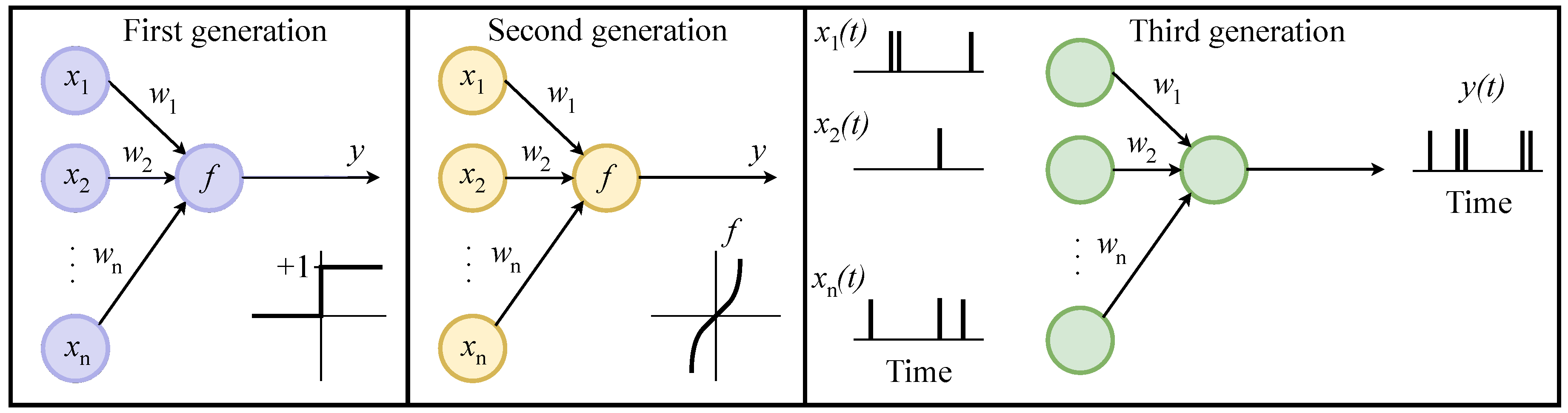
A brief description of various generations of neural networks is presented in Figure 1. The Rosenblatt perceptron belongs to the first generation. Its key feature is the binary activation function applied to the sum of input signals. However, by the end of the 1960s, it became clear that the capabilities of the perceptron are limited. Today’s wave of interest in neural networks comes from the invention of the continuous activation function. Examples of such functions are sigmoid, hyperbolic tangent, and ReLU [4]. All of them are non-linear, resulting in the complex nonlinear dynamics of the whole network. Unlike the first generation, the second one provides the ability to activate input neurons with analog signals. The second generation includes a lot of widely used solutions, such as deep learning, convolutional, and generative neural networks. Spiking neurons are the third generation of artificial neuron models, which closely mimic the dynamics of biological neurons [5]. Spiking neural networks (SNN) operate not with numbers but with one-time pulses (spikes) and their trains (bursts). The distribution of impulses over time makes it possible to encode and process the information. Neurons of the third generation also have an activation function, which, at a certain threshold of magnitude, generates an impulse, and thereafter the neuron is put to reset and a recovery period begins. SNNs are usually considered as having more potential than traditional ANNs due to the fact they outperform in terms of energy efficiency and are better suited to work with time-varying data [6]. However, the widespread use of SNNs is limited by several shortcomings. First, one needs to choose a method for representing data in the form of pulses [7]. A choice of encoding technique may be of key importance in terms of the network’s computational and energy costs [2]. Second, special learning methods are in demand for SNN. Finally, the most important limitation is modern von Neumann’s architecture itself, which is poorly adapted to reproduce the dynamics of spiking networks [8], which has led to the absence of time-efficient software solutions. However, with the development of dedicated architectures (e.g., memristor-based computers), this problem may be solved. Reservoir computing is a framework designed for computing based on the theory of recurrent neural network architecture, which maps input signals to higher-dimensional computational spaces through the dynamics of a fixed non-linear system called a reservoir [9]. After the input signal enters the tank, which is considered a “black box”, a simple readout mechanism is trained to read the state of the tank and output it in the desired format. The key advantage of this framework is that learning takes place only on the output layer since the reservoir dynamics are fixed. Reservoirs can be either physical or virtual. Virtual reservoirs are usually randomly generated to be similar to real neural networks. In virtual reservoirs, connections between blocks are randomized and remain unchanged throughout the computation process. The key factor for the correct operation of a reservoir neural network is the distinguishability condition: the system must be sufficiently distinguishable relative to the other patterns of behavior of reservoir neurons for different data classes [10]. While several types of reservoir computing exist, this work mainly focuses on the echo state network and the liquid state machine. The reservoir computing paradigm also aims to address the problem of the energy-inefficient operation of ANN [9]. Recall that a neural network containing more than one hidden layer is called a deep neural network [3]. To enforce the strength of the deep network, the recursive propagation of data through the network is performed. This is beneficial for overall accuracy, but the computational costs can be very high. Reservoir computing implements the opposite idea: the internal layers, which are called a reservoir, are not trained. They follow only their own dynamic properties affected by the input data and/or environment. Connection weights are deliberately optimized only at the output layer. The immutability of the hidden layers results in a huge advantage of RC: the facilitated learning process [3]. Figure 2 briefly represents the RC architecture.

Figure 1. Three generations of neural networks.

Figure 1. Three generations of neural networks.

RC and SNN, separately and in combination, have recently shown their advantages in solving many practical tasks. Morando et al. [11] used reservoir computing with automatic parameter optimization for proton-exchange membrane fuel cell (PEMFC) fault diagnostic. A possibility of online diagnostics without changing the system operating conditions with an error of less than 5% was shown. Zhang et al. [12] used pre-classified reservoir computing (PCRC) for the fault diagnosis of 3D printers equipped with a low-cost attitude sensor. An echo state network (ESN) was used as an RC for extracting faulty features and for the simultaneous classification of condition patterns. The authors demonstrated that the PCRC method has the best performance in comparison with RC, random forest (RF), support vector machine (SVM), and sparse auto-encoder (SAE). In [13], Kulkarni and Rajendran demonstrated the use of SNNs for handwritten digit recognition. In their experiments, an accuracy of 98.17% had been achieved on the MNIST dataset using the normalized approximate descent (NormAD) learning algorithm. Yan Z. et al. [14] used SNN for ECG classification. The authors provide a comparison between SNN and convolutional neural networks and show that SNN is much more energy efficient and, at the same time, demonstrates higher accuracy. Oikonomou et al. [15] successfully applied SNN in combination with deep learning in a robotic arm target-reach task. The authors of [16] used a probabilistic spiking response model (PSRM) with a multi-layer structure to classify bearing vibration data: the model was proven to be an effective tool for fault diagnosis.

However, in the current scientific literature, there is a lack of comparison between the second and third generations of neural networks with a reservoir architecture, which should be studied not only in terms of accuracy but also in learning and classification speed. In particular, the question arises: if ANNs are so expensive in terms of computing resources, can they be surpassed by SNNs on the same conventional computer?

Figure 2. Reservoir computing architecture.

Figure 2. Reservoir computing architecture.

Driven by this motivation, we designed the current study to perform the comparative evaluation of the second- and third-generation neural networks with reservoir architecture, namely, ESN and LSM, on the same datasets representing data from different types of sensors. The dependence of accuracy and speed on the number of neurons in the reservoir is evaluated. For the experimental study, we use the same hardware (personal computer), as well as the same open-source RCNet library.

The rest of the paper is organized as follows. In Section 2, we briefly describe ESN and LSM architectures, as well as datasets used in the study. In Section 3, the experimental results are presented. Section 4 discusses the obtained results and concludes the paper.

2. Materials and Methods

2.1. Neuron Models

The neurons in SNNs are built on mathematical descriptions of biological neurons (see Figure 3). There are two main groups of methods for modeling a neuron: either models based on conductivity (the Hodgkin–Huxley model, the Izhikevich model, the FitzHugh–Nagumo model, etc.) or threshold models (ideal, fluid, adaptive, exponential, and other integrate-and-fire models) [17]. One of the most common models for an SNN neuron is the leaky integrate-and-fire (LIF) model [18].

Figure 3. Biological neuron and its model used to build artificial neural networks.

Figure 3. Biological neuron and its model used to build artificial neural networks.

2.2. Learning Methods for Neural Networks

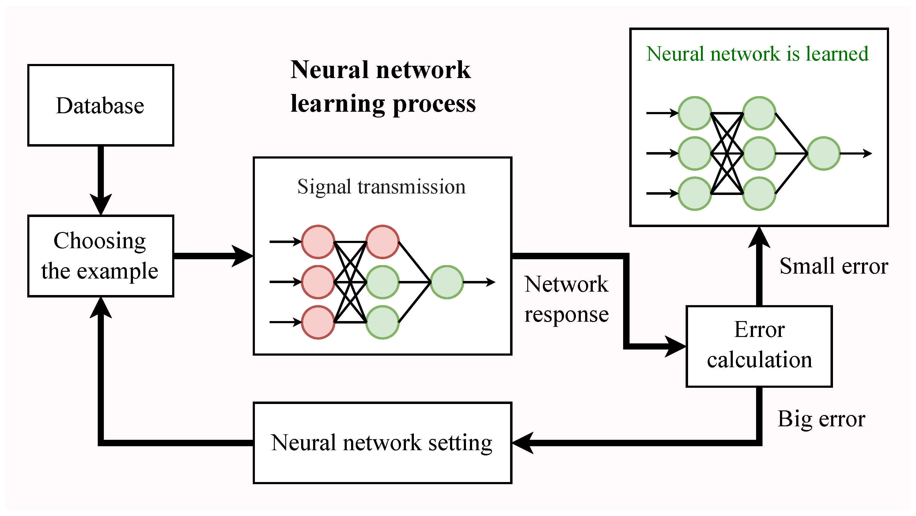
Learning methods of neural networks are divided into two main types: supervised learning and unsupervised learning. In some cases, elements of these two types are combined (reinforcement learning). Supervised learning implies that the learning material contains pairs of an example and the corresponding correct answer. A key aspect of learning is error calculation. This may be performed in two stages: forward or backward propagation of the error, respectively [19]. This learning method uses the so-called “chain rule” for functioning: after each pass through the network, an opposite pass is made in order to adjust its parameters. The result of running a neural network on a given training example is a numerical value that can be compared with the correct answer and evaluate the error. The estimation is made using a loss function, e.g., root mean square error (RMSE) or cross-entropy. Then, based on the value of this function, back-propagation is performed with the adjustment of the connection weights to get closer to the desired result of the network operation. Thus, the task of supervised learning can be described as finding the minimum estimated error (the result of the loss function). For this purpose, optimization algorithms are used. The number of learning process iterations may be referred to as the number of epochs and is often used as a comparative parameter. The authors of [20] show in detail how supervised learning is applied to spiking neural networks (Figure 4).

Figure 4. Supervised learning.

Figure 4. Supervised learning.

2.2.1. Echo State Network

The echo state network (ESN) [21] is a type of reservoir computing that uses a recurrent neural network with a sparsely connected hidden layer. Weights of connections between hidden neurons are randomly determined and fixed. The weight of the output neuron connections can be changed through training, so specific temporal patterns created by the reservoir can be interpreted. ESN is a second-generation neural network.

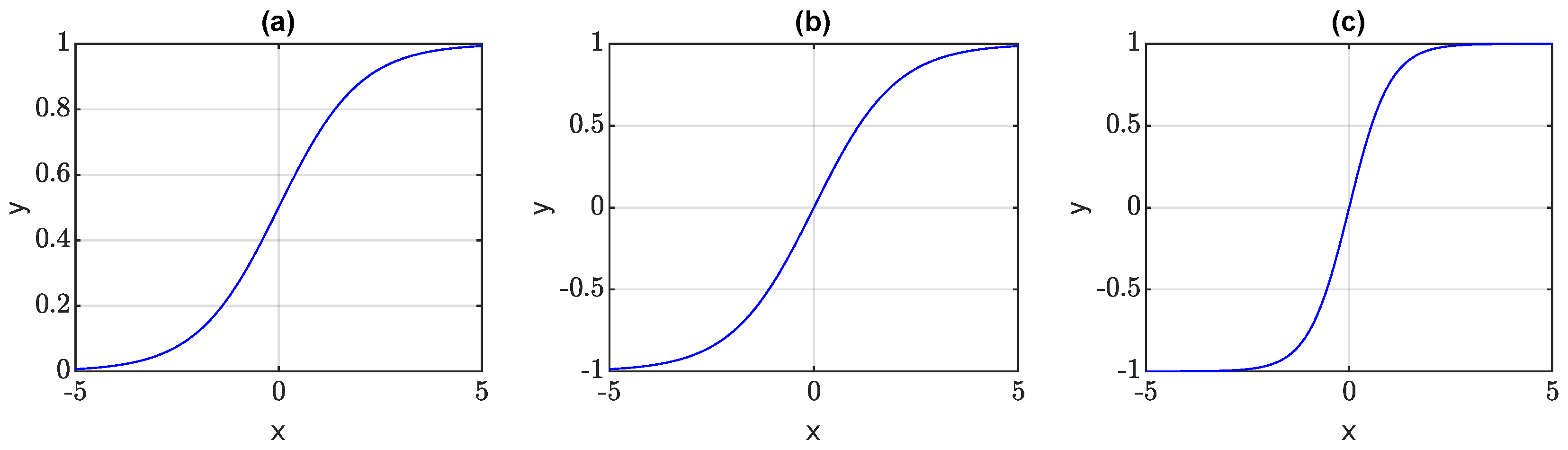
In paper [22], experimental data on activation functions’ performance was obtained. The tested neural networks were using a feedforward multilayer-perceptron architecture with one hidden layer. Firstly, there were 10 neurons in the hidden layer, and secondly there were 40 neurons. Five activation functions were tested, three of them being uni-polar sigmoid, bi-polar sigmoid, and hyperbolic tangent (Figure 5). Though the learning rates of these functions were not the fastest, their accuracy greatly exceeded the results obtained from the other two functions: conic section and the radial basis function. The hyperbolic tangent (tanh) showed the best accuracy rate with both 10 and 40 neurons. Based on this result, tanh was chosen as an activation function for ESN.

A hyperbolic tangent function can be expanded as the ratio of the half-difference and half-sum of two exponential functions in the points x and $-x$ as follows:

$$\begin{array}{cc}\hfill & tanh\left(x\right)=\frac{e^x-e^{-x}}{e^x+e^{-x}};\hfill \end{array}$$

(1)

2.2.2. Liquid State Machine

The liquid state machine (LSM) [23] is a type of reservoir computing that implements spiking reservoir architecture. The “soup” of a large number of recurrently connected neurons forms a large variety of non-linear functions. With a sufficient variety of these non-linear functions, it becomes possible to obtain linear combinations, respectively, to perform any mathematical operations necessary to achieve a given goal, such as speech recognition or computer vision. The name comes from an analogy with a stone that has fallen into a liquid: it creates circles on its surface. Thus, the input (movement of the falling stone) was translated into a spatiotemporal pattern of fluid movement (circles).

For LSM, an adaptive exponential integrate-and-fire model was chosen. According to [24], this model is both biologically accurate and simple enough to potentially show good results in terms of both accuracy and speed.

The traditional integrate-and-fire model combines linear filtering of input currents with a strict voltage threshold. Exponential integrate-and-fire neurons allow for the replacement of the strict voltage threshold by a more realistic smooth spike initiation zone, and the addition of a second variable allows for the inclusion of subthreshold resonances or adaptation [24]. An integrate-and-fire model with adaptation is defined as:

$$\begin{array}{cc}\hfill & C\frac{dV}{dt}=f\left(V\right)-w+I;\hfill \end{array}$$

(2)

where C is the membrane capacitance, w is an adaptation variable, I is the synaptic current, V is the membrane potential, and $f\left(V\right)$ is a function that characterizes the spiking mechanism and is taken as a combination of linear and exponential functions:

$$\begin{array}{cc}\hfill & f\left(V\right)=g_L(V-E_L)+g_L{\mathrm{\Delta }}_{T}exp\left(\frac{V-V_T}{{\mathrm{\Delta }}_T}\right);\hfill \end{array}$$

(3)

where $g_L$ is the leak conductance, $E_L$ is the resting potential, ${\mathrm{\Delta }}_T$ is the slope factor, and $V_T$ is the threshold potential.

The resulting model is called adaptive exponential integrate-and-fire [24].

2.3. Libraries, Programming Languages, and Hardware

The RCNet library by Oldřich Koželský was chosen for implementing both ESN and LSM. The mathematical background of the library is taken from the book by Gerstner et al. [25], summarizing the basics of modern computational and theoretical neuroscience. This library provides features such as converting analog signals to spikes, which can be used in further studies of the applicability of spiking neural networks.

One of the main features of the RCNet library is that the reservoir architectures of both generations of neural networks are built identically, up to the possibility of combining two generations of neurons in different layers without loss of functionality. In the RCNet library, input and hidden layers are combined in a single component NeuralPreprocessor, which, together with ReadoutLayer, form StateMachine, an instance of a complete neural network. The number of input layer neurons is determined automatically by the length of input data. The number of hidden layer neurons is defined freely; in our study, it was chosen as the number from 50 to 250 with the step of 50. The number of output layer neurons is defined according to the number of data classes.

The programming language used was C#, and the development environment was Visual Studio 2022. All of the computations were performed using the PC with the following configuration.

• Model: ASUS ROG STRIX G15 G513IH-HN002;
• CPU: AMD Ryzen 7 4800H 8 cores 2.9-4.2 GHz;
• GPU: GeForce GTX 1650;
• RAM: DDR4 8 Gb;
• Storage device: SSD M.2 PCIe 512 Gb.

2.4. Datasets

2.4.1. ETU Bearing Dataset

This dataset was created especially for research and development of electric motor faults diagnosis systems based on the phase currents analysis. It was named after Saint Petersburg Electrotechnical University (ETU), where the data was collected.

For a long time, the main instrument for diagnosing motor faults was the accelerometer capturing the vibration signals. Vibration signatures of faults are well-recognizable, even in presence of the background noise. However, the disadvantage of measuring vibration with accelerometers is the need for additional sensors and signal processing units, which is not always reasonable or even possible. 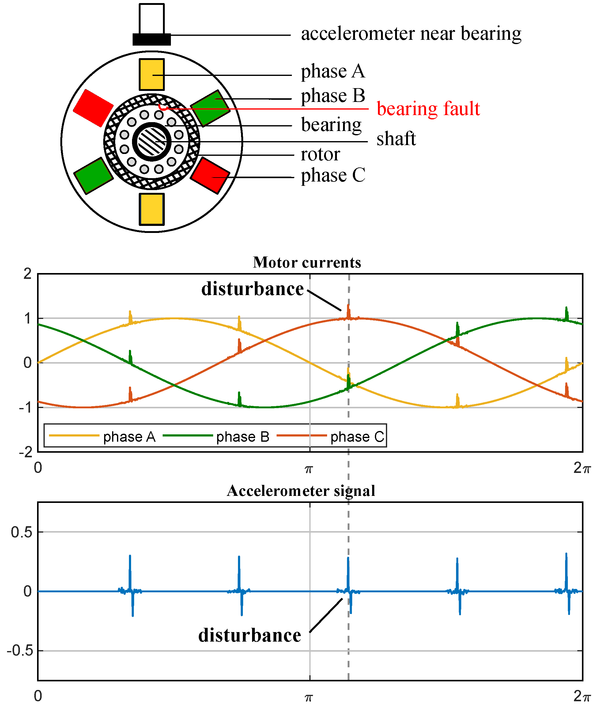The authors of [26] first proposed the idea to consider the rotor of the electric motor as an accelerometer itself, which makes possible the application of vibration analysis methods for current data without external sensors. The idea of phase current diagnostics and the relationship between signals from the accelerometer and current sensors is presented in Figure 6: a mechanical defect can be detected not only by the accelerometry but also with current measurements as the similar disturbances are induced in the phase current signals. Theoretically, a single-phase signal should be sufficient for analysis purposes. The authors of [27] first used this approach to detect motor bearing faults.

The classical bearing fault detection algorithms are based on spectrum analysis. It is known that different bearing faults induce specific mechanical frequencies in the signal spectrum. For the rotor frequency $F_R$, the ball diameter $D_b$, the pitch diameter $D_c$, the number of rolling elements $N_B$, and the ball contact angle $\beta$, mechanical frequencies for the faults will be:

$$\begin{array}{cc}\hfill & F_I=\frac{N_B}{2}{F}_R(1+\frac{D_{b}cos\beta }{D_c});\hfill \end{array}$$

(4)

$$\begin{array}{cc}\hfill & F_O=\frac{N_B}{2}{F}_R(1-\frac{D_{b}cos\beta }{D_c});\hfill \end{array}$$

(5)

$$\begin{array}{cc}\hfill & F_B=\frac{D_c}{D_b}{F}_R[1-{\left(\frac{D_{b}cos\beta }{D_c}\right)}^2];\hfill \end{array}$$

(6)

where $F_I$ is the inner race fault frequency, $F_O$ is the outer race fault frequency, and $F_B$ is the ball fault frequency.

The commonly used approach of evaluating the frequencies of defects is based on the representation of vibration as a torque component that generates a chain of frequency components $F_{be}$ in the current signal.

To perform the analysis of signal with frequencies $F_{be}$, it is first required to separate the mechanical characteristic signal from the carrier f, which can be done in different ways, for example, by bandpass filtering of the signal.

With all of its advantages, phase current analysis possesses its difficulties and limitations. The exact characteristics of the motor as a sensor are unknown, and the current signals induced from mechanical defects are weak, and they must be detected in the presence of a powerful component–the supply frequency. Additionally, the motor itself, even in good condition, generates a wide range of harmonics that must be distinguished from mechanical signals. Immovilli et al. [28] conclude that only defects characterized by relatively low mechanical frequency can be detected in such a way. However, the recent development of machine learning and neural networks has led to promising results. Wagner and Sommer [29] show that phase current analysis by a multilayer perceptron in the feature space makes it possible not only to recognize bearing faults at different motor rotation speeds but also to adapt the trained model to conditions different from those where the model learning was performed.

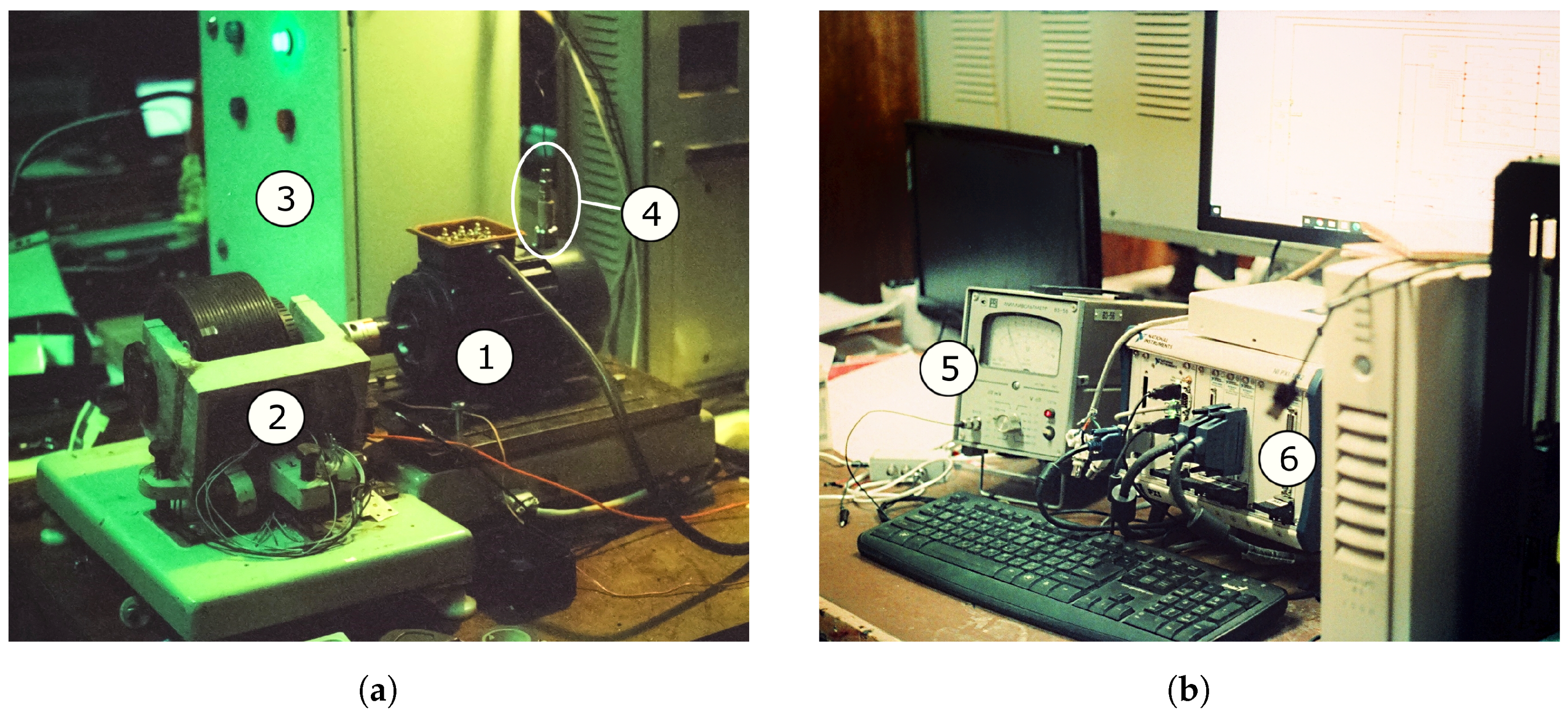
Figure 7 presents the experimental bench for ETU bearing dataset recording. It includes a 0.75-kW asynchronous motor (AIR71V4U2) and electromagnetic brake, connected via the clutch. The bench allows for simulating the nominal state of electric motor operation, as well as the overload mode. Currents are acquired by the Hall effect sensors LTS 25-NP with a frequency band of up to 100 kHz. Sensor data is collected through the SCB-68A analog input/output unit. The acquired signals are transferred to the 16-bit ADC of the NI PXI-6123 board, where they are digitized with a sampling rate of 10 kS/s. The digitized signals are processed and recorded into TDMS files using the NI PXI-8106 device and NI LabVIEW 2020 software.

Table 1 presents the content of the dataset used for the study. The motor had no load and ran at a speed of 1498 RPM. The bearing with artificially induced inner race fault was installed to record data for broken bearing. Each of the 10 recordings lasts for 60 s, and for the dataset, 50 pieces (each 5 s long) were randomly taken from every phase current A waveform. At a pre-processing stage, the waveforms were cleared from the supply frequency and bandpass filtered to leave the frequency content only in the range from 1 Hz to 260 Hz.

The difficulty of the classification task in this dataset is that the introduced bearing fault had not noticeably affected the phase currents due to strong mechanical vibrations in the electromagnetic brake bearings and inaccurate alignment of the motor and brake axes. Thus, the collected data present a challenge for classification algorithms.

Table 1. Classes of ETU Bearing Dataset for 1498 RPM.

Classes	Number of Points in Waveforms	If the Class Is Used in This Work	Number of Segments of 50,000 Points Length for Training	Number of Segments of 50,000 Points Length for Testing
Healthy	6,000,000	yes	30	20
Broken	6,000,000	yes	30	20

Table 1. Classes of ETU Bearing Dataset for 1498 RPM.

Classes	Number of Points in Waveforms	If the Class Is Used in This Work	Number of Segments of 50,000 Points Length for Training	Number of Segments of 50,000 Points Length for Testing
Healthy	6,000,000	yes	30	20
Broken	6,000,000	yes	30	20

2.4.2. Bearing Data Center Dataset

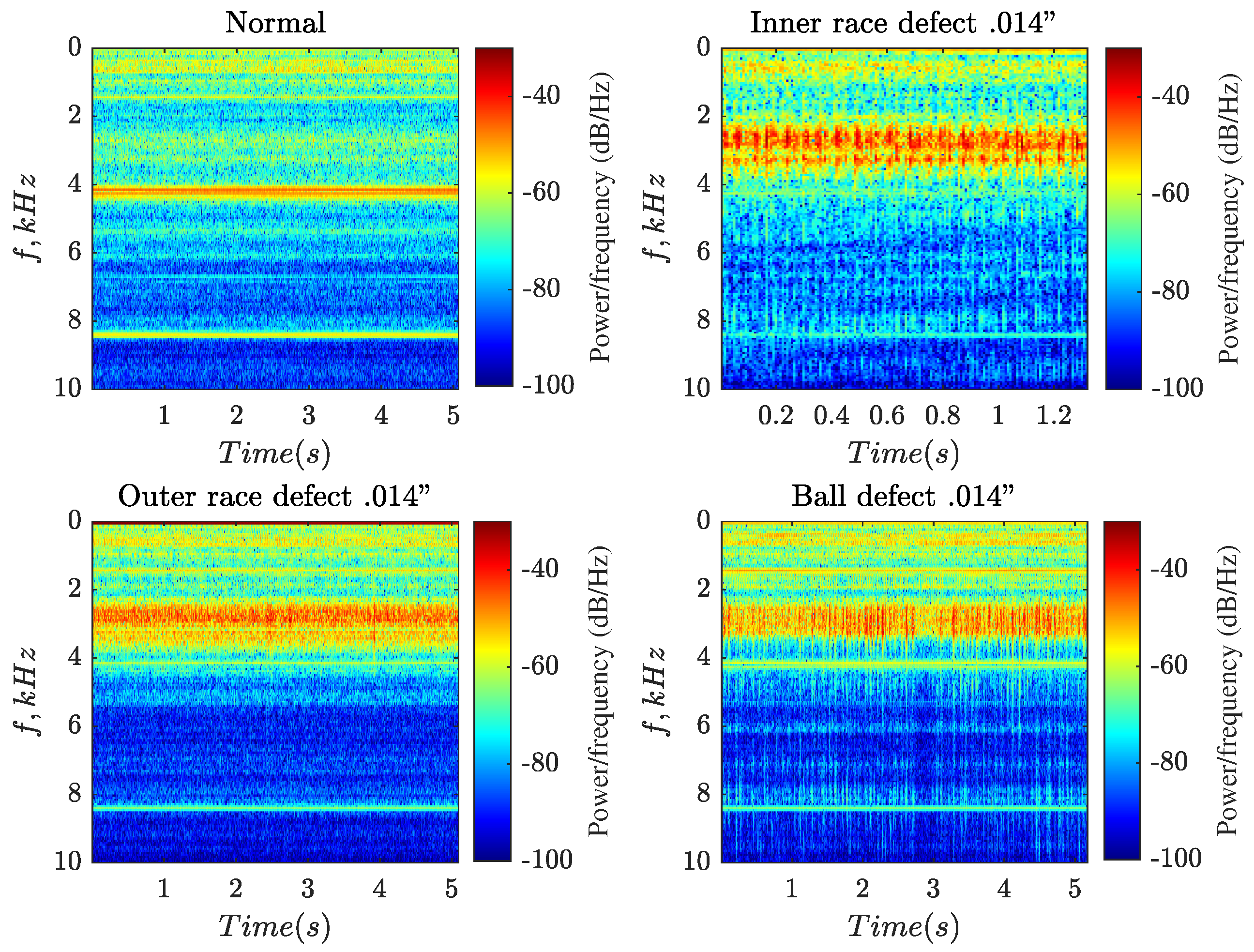
The popular dataset by [30] contains ball bearing test data for normal and faulty bearings. Experiments were conducted using a 2-horse-power reliance electric motor. The acceleration data was recorded at locations that were near and remote from the motor bearings. There are ten classes of data: one for normal bearing and nine for three types of fault (ball defect, inner race defect, and outer race defect) and three degrees of damage–refer to

Table 2. Classes of bearing data center dataset for drive end accelerometer and 1797 RPM speed.

Classes	Number of Points in Waveform	If the Class Is Used in This Work	Number of Segments of Length 2400 Points for Training	Number of Segments of Length 2400 points for Testing
Normal	243,938	yes	50	50
B007	244,739	yes	50	50
B014	249,146	yes	50	50
B021	243,938	yes	50	50
IR007	243,938	yes	50	50
IR014	63,788	yes	50	50
IR021	244,339	yes	50	50
OR007	244,739	yes	50	50
OR014	245,140	yes	50	50
OR021	246,342	yes	50	50

. Before feeding the data into the neural network, the waveform is converted into a spectrogram using short-time Fourier transform (STFT), a technique that is widely used in signal-processing tasks such as human voice detection and machine pattern recognition [31] (see Figure 8 for examples and Section 2.5 for deeper explanation).

2.4.3. Gearbox Fault Diagnosis Dataset

The last used dataset is [32] available at Kaggle online platform. It includes the vibration data recorded from SpectraQuest’s Gearbox Fault Diagnostics Simulator and contains data on healthy and broken tooth conditions. The dataset has been recorded with the help of four vibration sensors (A1–A4) placed in four different directions (see Table 3). Load values vary from 0 to 90 percent. For this work, the load value was taken as 90 percent, and measurements from sensor A2 were used as samples.

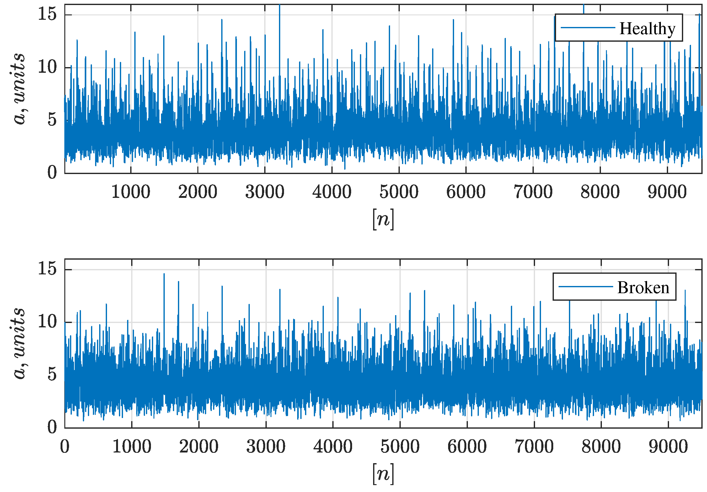
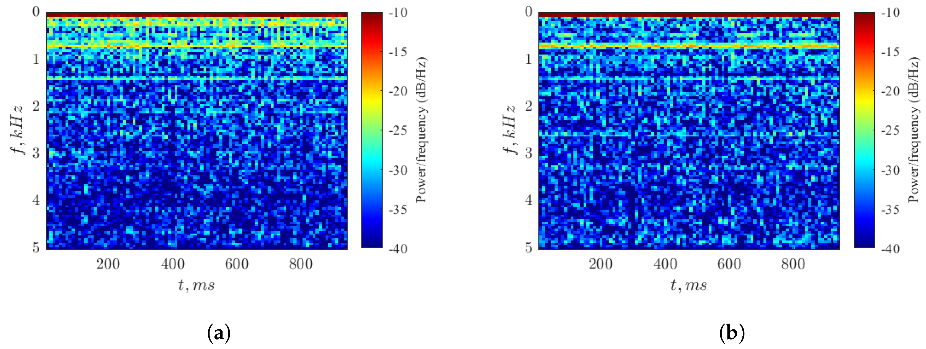
In Figure 9, examples of records from the dataset are given. Samples present vibration waveforms taken from the accelerometer, with values in conventional units. There are no noticeable signs of a defect in the waveforms, so it is necessary to apply a preliminary analysis to enable the neural network to find the defect features. The spectrograms of healthy and broken gearboxes are shown in Figure 10.

Figure 9. Examples of data samples in gearbox fault diagnosis dataset. Recordings from accelerometer A2.

Figure 9. Examples of data samples in gearbox fault diagnosis dataset. Recordings from accelerometer A2.

Figure 10. Healthy (a) and broken (b) gearbox vibration spectrograms for load value 90. Visualization is performed in the assumption of the 10 kS/sec rate.

Figure 10. Healthy (a) and broken (b) gearbox vibration spectrograms for load value 90. Visualization is performed in the assumption of the 10 kS/sec rate.

Table 3. Classes of gearbox dataset for load value of 90.

Classes	Number of Points in Waveform	If the Class is Used in This Work	Number of Segments of Length 10,000 Point for Training	Number of Segments of Length 10,000 Point for Testing
Healthy A1	106,752	no	-	-
Broken A1	105,728	no	-	-
Healthy A2	106,752	yes	50	50
Broken A2	105,728	yes	50	50
Healthy A3	106,752	no	-	-
Broken A3	105,728	no	-	-
Healthy A4	106,752	no	-	-
Broken A4	105,728	no	-	-

Table 3. Classes of gearbox dataset for load value of 90.

Classes	Number of Points in Waveform	If the Class is Used in This Work	Number of Segments of Length 10,000 Point for Training	Number of Segments of Length 10,000 Point for Testing
Healthy A1	106,752	no	-	-
Broken A1	105,728	no	-	-
Healthy A2	106,752	yes	50	50
Broken A2	105,728	yes	50	50
Healthy A3	106,752	no	-	-
Broken A3	105,728	no	-	-
Healthy A4	106,752	no	-	-
Broken A4	105,728	no	-	-

2.5. Datasets Pre-Processing

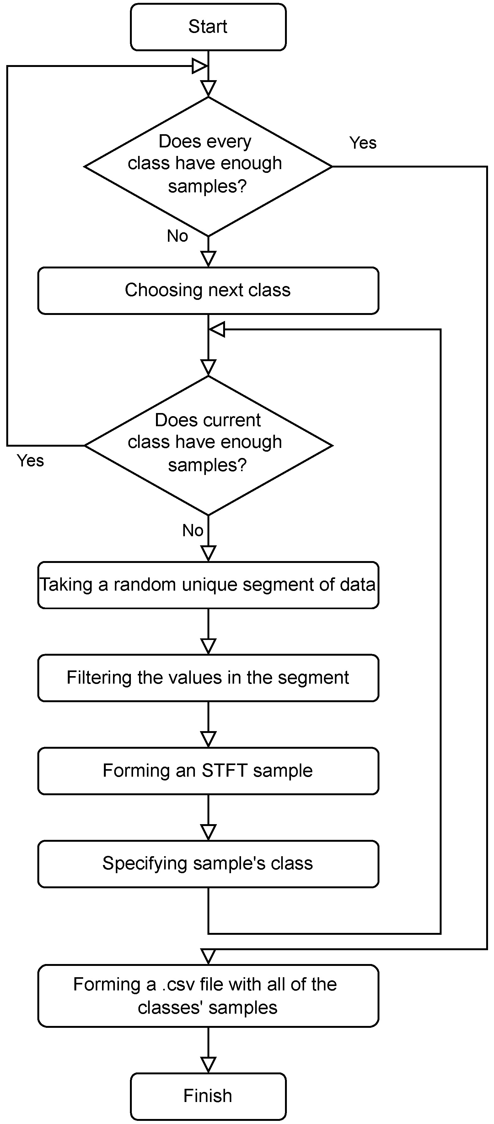
All three datasets consist of long recordings. In order for the classification process to be effective, not all of the data have to be worked with. The data must be mapped into a feature space, the number of which should not exceed the order of ${10}^3$. As a feature extraction algorithm, we utilized fast and efficient short-time Fourier transform (STFT). The amount of short signal segments is equal for every class of data and is 10 samples at minimum. The full process of a dataset pre-processing is demonstrated in Figure 11.

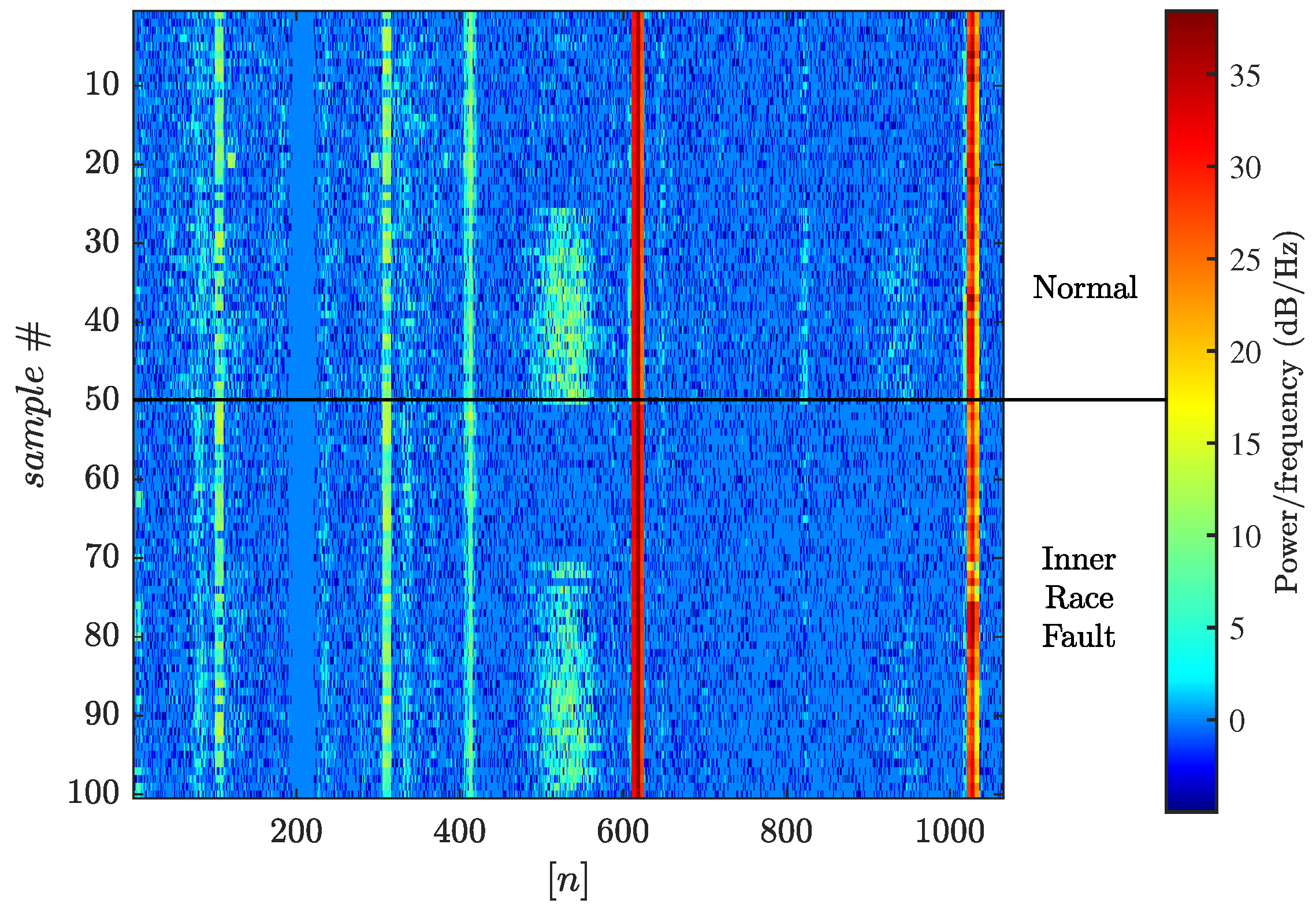
Examples of the data ready for feeding into the RCNet neural network are represented as images and are shown in Figure 12 and Figure 13. Every line corresponds to one sample of the training or testing dataset. Depending on the settings, the repeated patterns of the spectrogram appear in the dataset. It can be seen that the repetitions are slightly different, which is a consequence of the variability of the spectrum of the analyzed waveforms.

Figure 11. Order of operations in forming a dataset.

Figure 11. Order of operations in forming a dataset.

2.6. Comparative Evaluation

To compare the effectiveness of neural networks with each other, three parameters were identified: training time, testing time, and accuracy. Accuracy was calculated as the ratio of correct network classifications to their total number. These parameters were used to analyze the speed and accuracy of the networks under test.

The number of neurons in the hidden layer (reservoir) was set as a variable parameter. Thus, the dependence of the three previously described parameters on the volume of the reservoir was established.

Hyperparameters, when possible, were chosen to be equal for ESN and LSM. The main parameters were set as follows: number of training attempts was 5; the number of epochs within one attempt was 400. Thus, each training attempt had a sufficient number of epochs to create a potentially optimal neural network, and, due to several training attempts, the influence of the randomness factor was reduced, as the best configuration was chosen automatically.

3. Results and Discussion

3.1. Training Time

As a result of testing, the comparative data obtained are shown in Figure 14 (logarithmic axis scale) and

Table 4. Comparative training time values.

Number of Neurons	ETU Bearing–ESN, sec	ETU Bearing– LSM, sec	Bearing Data Center– ESN, sec	Bearing Data Center–LSM, sec	Gearbox Fault Diagnosis–ESN, sec	Gearbox Fault Diagnosis–LSM, sec
50	47.353	543.39	114.633	373.073	21.896	180.414
100	48.093	592.891	149.854	628.645	24.776	210.002
150	61.192	680.536	198.986	934.213	27.655	258.775
200	76.618	819.313	243.586	1402.423	32.759	306.776
250	86.761	1023.68	306.056	1985.818	27.649	371.039

. One may see that a spiking neural network requires an order longer time to train for a dataset with a small number of classes. However, in the case of a dataset with a large number of classes (bearing data center), the difference in training time is times, not orders. Figure 14 shows the training time in the case of different datasets vs. the number of neurons N. For ESN, this value depends on N almost linearly, but for LSM, this dependence is exponential (notice the logarithmic scale of Y axis).

3.2. Testing Time

As a result of testing, the comparative data obtained are shown in Figure 15 (logarithmic axis scale) and presented in

Table 5. Comparative testing time values.

Number of neurons	ETU Bearing–ESN, sec	ETU Bearing– LSM, sec	Bearing Data Center–ESN, sec	Bearing Data Center–LSM, sec	Gearbox Fault Diagnosis–ESN, sec	Gearbox Fault Diagnosis–LSM, sec
50	10.512	153.374	10.87	282.399	11.572	156.648
100	11.231	333.218	16.197	536.306	14.684	203.9
150	14.51	301.042	23.358	814.411	16.932	245.516
200	19.453	367.4	33.259	1263.825	18.923	287.556
250	25.124	505.474	51.35	1694.431	20.647	341.287

. The spiking neural network requires an order longer time for testing in all cases. In Figure 15, the testing time vs. the number of neurons N is plotted. One can see that the testing time of ESN increases exponentially with the growth of N in the case of 2 of 3 datasets, but for LSM these curves are more linear.

3.3. Accuracy

As a result of testing, the comparative data obtained are shown in Figure 16 and presented in

Table 6. Comparative accuracy values.

Number of Neurons	ETU Bearing–ESN, Percent	ETU Bearing– LSM, Percent	Bearing Data Center–ESN, Percent	Bearing Data Center– LSM, Percent	Gearbox Fault Diagnosis–ESN, Percent	Gearbox Fault Diagnosis–LSM, Percent
50	67.5	85	51	100	81	100
100	75	80	50	100	86	100
150	72.5	90	53.8	100	82	100
200	72.5	82.5	60.8	100	90	100
250	65	87.5	55.2	100	89	100

. Figure 16 shows the dependence of accuracy on the number of neurons N. One may see that for both architectures, the increase of N from 50 to 250 usually leads to an increase of accuracy up to 10%. Nevertheless, in the case of the ETU bearing dataset and ESN, accuracy does not increase. This may be considered a case of overtraining as the features presented in the dataset cannot be captured by ESN, in contrast to LSM.

3.4. Discussion

Generalizing the obtained results, we have found a large superiority of SNN over ANN in the spectrogram’s recognition accuracy, which is one of the important insights of our study. For all three considered datasets, SNN provides much fewer errors than ANN. The use of a small amount of samples with specific patterns for teaching may result in recognition accuracy of SNN up to 100%, while ANN fails.

With that, we should list some limitations of the approach. First, we cannot generalize our results to all ANNs. We compared SNN to ANN, whose architecture differed in the dynamics of individual neurons but not in the structure of layers or the type of learning. Second, we believe that SNN would show their best performance in dedicated neuromorphic hardware but not in conventional computers. Figure 14 and Figure 15 clearly show that training and testing times increase dramatically when using SNN, up to 10 times and higher, in comparison with ANN.

4. Conclusions

In this study, we performed a comparative evaluation of artificial and spiking neuron networks with reservoir architecture. The research was carried out using three datasets for solving the following tasks: ball bearing fault detection using an induction motor phase currents signals (ETU bearing dataset), ball bearing fault detection using signals from an accelerometer (bearing data center dataset), gearbox broken tooth detection using signals from the accelerometer (gearbox fault diagnosis dataset). The spectral analysis, namely, STFT, was used for feature extrication from the waveforms and the preparation of samples for learning and tests.

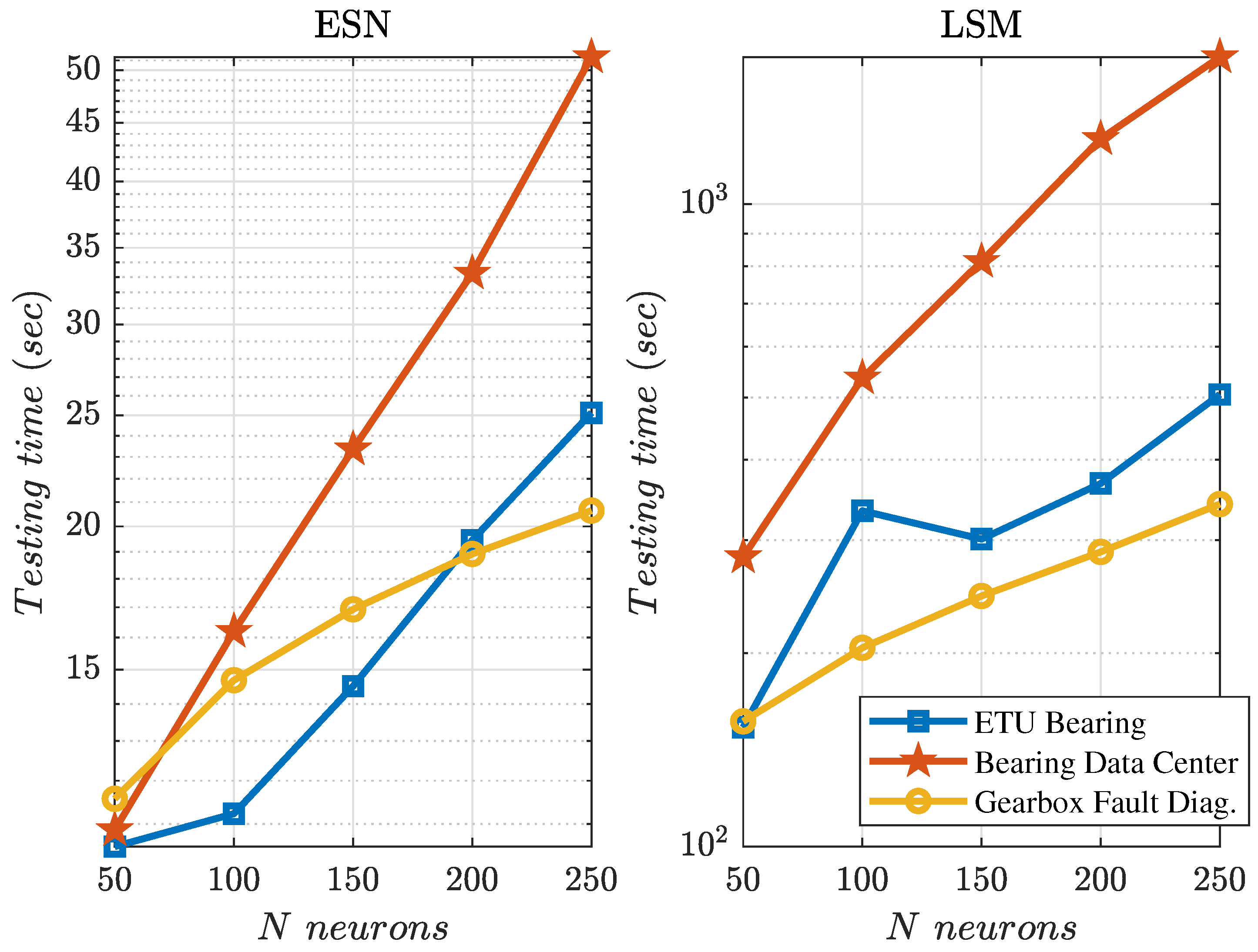
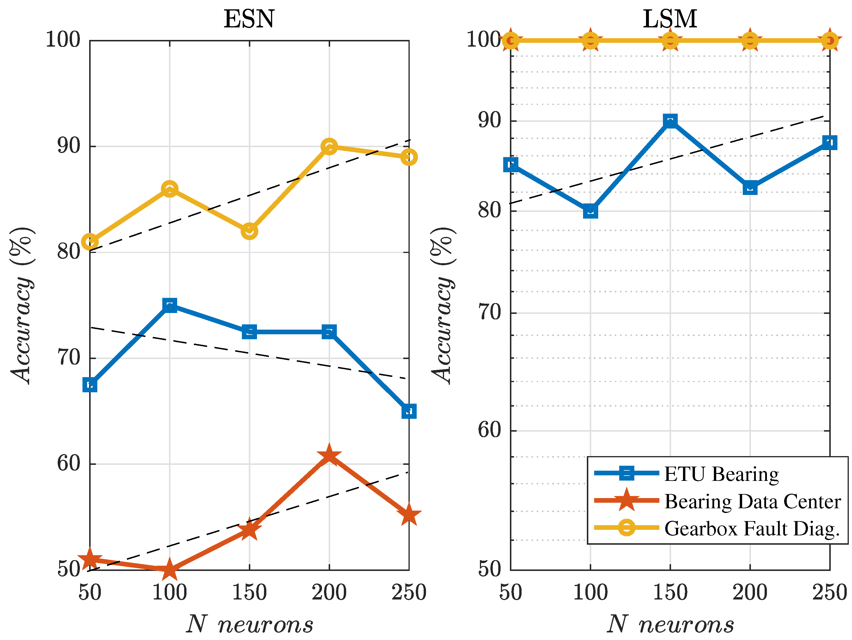
The experimental results show that the second-generation reservoir architecture (ESN) is significantly inferior to the third-generation (LSM) in terms of accuracy (11–64%). The training time of the third generation neural network (LSM) exceeds those for ESN by 2.2–10 times, and an operating time by one order (12–25 times). The brief comparison of numerical values for ESN and LSM is shown in Table 7.

Additionally, we obtained some observations on the neural network training and testing times and accuracy in the dependence on the number of neurons N. For ESN, training time linearly grows with an increase of N but testing time grows rather exponentially. For LSM, this was found to be converse. Additionally, with growths of N from 50 to 250, the total increase of accuracy for both architectures was not more than 10%. In the case of the ETU bearing dataset, the accuracy of ESN even decreased.

Table 7. Comparative peak values.

	Dataset 1: ETU Bearing	Dataset 2: Bearing Data Center	Dataset 3: Gearbox Fault Diagnosis
3rd gen overcame 2nd gen in peak accuracy	20%	64.47%	11.11%
2nd gen overcame 3rd gen in peak training time	1047.53%	225.45%	723.96%
2nd gen overcame 3rd gen in peak testing time	1359.04%	2497.97%	1253.68%

Table 7. Comparative peak values.

	Dataset 1: ETU Bearing	Dataset 2: Bearing Data Center	Dataset 3: Gearbox Fault Diagnosis
3rd gen overcame 2nd gen in peak accuracy	20%	64.47%	11.11%
2nd gen overcame 3rd gen in peak training time	1047.53%	225.45%	723.96%
2nd gen overcame 3rd gen in peak testing time	1359.04%	2497.97%	1253.68%

We may conclude that LSM architecture is able to show exceptional accuracy for fault detection in electrical and mechanical machines. However, due to its high computational demands, the use of LSM for real-time diagnostics may be limited. For a wider application of third-generation neural networks, it is necessary to continue the search for solutions that would reduce the time of their work and training. One of the promising directions in this area may be the creation of hardware architectures based on memristive elements.