Article

Analysis of the Numerical Solutions of the Elder Problem Using Big Data and Machine Learning

by
Roman Khotyachuk
1,* and
Klaus Johannsen
2
1
Faculty of Mathematics and Natural Sciences, University of Bergen, 5020 Bergen, Norway
2
NORCE Norwegian Research Center AS, 5008 Bergen, Norway
*
Author to whom correspondence should be addressed.
Big Data Cogn. Comput. 2023, 7(1), 52; https://doi.org/10.3390/bdcc7010052
Submission received: 27 December 2022 / Revised: 28 February 2023 / Accepted: 15 March 2023 / Published: 20 March 2023
(This article belongs to the Topic Big Data and Artificial Intelligence)

Abstract

:
In this study, the numerical solutions to the Elder problem are analyzed using Big Data technologies and data-driven approaches. The steady-state solutions to the Elder problem are investigated with regard to Rayleigh numbers ( R a ), grid sizes, perturbations, and other parameters of the system studied. The complexity analysis is carried out for the datasets containing different solutions to the Elder problem, and the time of the highest complexity of numerical solutions is estimated. An approach to the identification of transient fingers and the visualization of large ensembles of solutions is proposed. Predictive models are developed to forecast steady states based on early-time observations. These models are classified into three possible types depending on the features (predictors) used in a model. The numerical results of the prediction accuracy are given, including the estimated confidence intervals for the accuracy, and the estimated time of 95% predictability. Different solutions, their averages, principal components, and other parameters are visualized.

1. Introduction

Density-driven flows in porous media are frequently observed in natural and technical systems. They are caused by different densities of mixing fluids or changes in their temperature, and sometimes by a combination of these two factors. Such fluid and thermal processes have significant environmental and economic impacts.
The Elder problem is the example of density-driven flows induced by variations in density. This type of flow appears in many practical cases, such as freshwater–saltwater interactions, heat transfer, and carbon dioxide sequestration. John Elder provided an original formulation of this problem for thermal convection flows [1,2]. Later, the equations mathematically identical to the Elder problem were used to describe other physical processes. For example, Voss and Souza (1987) [3] reformulated them for the case of saltwater–freshwater flows. In addition, there is a connection between the Elder problem and the broader class of other problems that describe convection in porous media [4].
The numerical modeling of flows in porous media is used, in addition to its undoubtedly high theoretical value, to predict their behavior in a number of important practical cases, such as risk assessment, water resource management, geothermal reservoir study, and evaluating the safety of reservoirs for radioactive waste. Such modeling is challenging because of the high variability in flow processes, the non-linearity of governing equations, and the wide range of time and space domains where a problem is solved numerically.
In the present study, we analyze large sets (ensembles) of numerical solutions to the Elder problem using Big Data technologies and machine learning (ML) techniques.
The paper is organized as follows. In Section 2, we describe the Elder problem itself, the governing partial differential equations (PDEs) and their numerical models, scientific questions, and some other related subtasks. In Section 3, we briefly describe the methods, approaches, and software used in this work. In Section 4, we present and discuss our results, including unperturbed and perturbed simulations, and the identification and visualization of the properties of numerical solutions, complexity analysis, and predictive modeling of the Elder problem.

2. Models and Scientific Questions

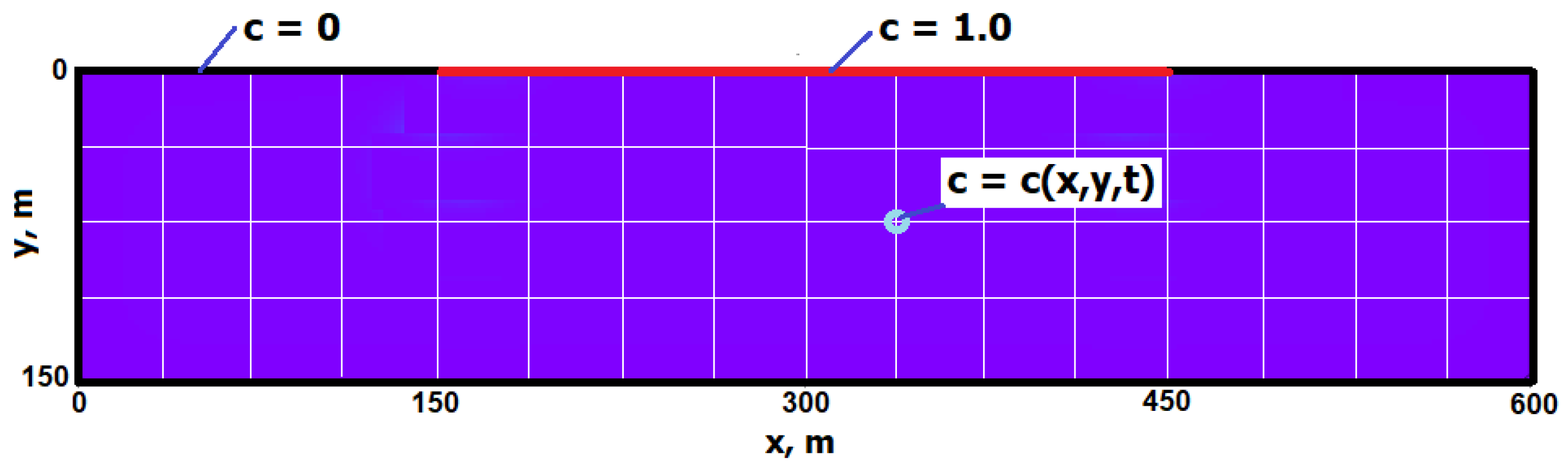
2.1. The Elder Problem

The governing equations for density-driven flows in porous media are derived from the mass-conservation principles:
n ρ t = ρ ν n ρ ω t + ρ ω ν ρ D m ω = 0 ,
where ω is the salt mass fraction, ρ is the density, n is the porosity, D m is the molecular diffusion coefficient, and ν is the average mass velocity. ν is given by Darcy’s law:
ν = K μ ( ρ ρ g ) ,
where K denotes permeability, μ denotes viscosity, and g denotes the gravity vector. Density is obtained from the ideal mixing relation:
1 ρ = ( 1 ω ω m a x ) 1 ρ m i n + ω ω m a x 1 ρ m a x ,
where ω m a x is the maximum salt mass fraction, ρ m i n is the minimum density, and ρ m a x is the maximum density. In the present work, we use salt concentrations c in a non-dimensional form, and it is rescaled to the range c = 0 , 1 .
The geometry and boundary conditions of the Elder problem are provided in Figure 1, and physical parameters are provided in Table 1.
The Rayleigh number is a measure of the strength of the non-linearity existing in a system studied. It is widely used to characterize the regime of fluid flows. In the case of the Elder problem, it is defined as follows:
R a : = K ( ρ m a x ρ m i n ) g h D m μ n ,
where h = 150 m is the characteristic length of the problem (see Figure 1).
The Elder problem, as a dynamical system described by the system of Equation (1), is known to have three stable steady-state solutions. They are obtained asymptotically when t . If we visualize these solutions using contour plots at each time t, we can notice some concentration fields with the shape of a human finger. The process typically starts with more than two “fingers” at t = 1–2 years; small fingers are merged into larger ones, and at t , the process converges to a solution with one, two, or three fingers, depending on physical parameters, initial conditions, etc. These solutions are called one-, two-, or three-finger steady-state solutions. They are usually denoted S1, S2, or S3, respectively [5,6]. These three solutions are depicted in Figure 2. S1 and S2 solutions are also mentioned as upwelling and downwelling solutions [2], respectively. The solutions at t = 0 are called initial solutions, and the solutions in 0 < t < are called transient solutions.
Fingering can be defined as the process of appearing, growing, and merging small fingers into larger ones. It is highly dependent on the physical parameter of the studied system, perturbations, etc. The one-, two-, and three-finger solutions may look quite similar at an early time (Figure 2, see the solutions at t = 2 years). However, they start to change very significantly over the next periods, and finally become S1, S2, or S3 solutions at t . In Section 4.3, we will describe our approach and the results in identifying transient fingers and in estimating their positions and strength.
For the given initial conditions of the Elder problem, the correct steady-state solution is very likely the S1 or S2 solution, although a proof does not exist. If the initial conditions of the problem are slightly altered, the S1 solution could be the result instead of the expected S2 solution and vice versa: the S2 instead of the expected S1 solution. If the setup of the problem is significantly altered, the three-finger solution (S3) could also arise, but this is a rare situation.

2.2. Existing Approaches to the Elder Problem

The numerical solutions of PDEs that describe the Elder problem have been investigated by many researchers. As mentioned above, Elder originally reported such solutions after his thermal convection experiments in porous media [7]. They have been studied by other researchers (Voss and Souza 1987 [3]; Johannsen 2003 [5]; Simmons et al., 1999 [8]; Van Reeuwijk et al., 2009 [9]). They focused basically on obtaining numerical solutions to the Elder problem using different numerical solvers for Equations (1), and investigated the numerical stability and sensitivity of the obtained solutions. There was some controversy in the results reported by different researchers; that is, about which solution is the right one. It was associated with the number of fingers in a steady state (S1, S2, or S3) and was caused by different numerical methods applied to solve the PDEs, or different parameters of the problem.
This discussion started with Elder’s results (1967) [1]. He provided a single-finger solution for the case of R a = 400 in dimensionless time t = 0.1 , i.e., near steady state. Then, Voss and Souza (1987) [3] reproduced Elder’s one-finger solution using the SUTRA model [10]. This S1 solution was considered correct for the next eight years until Oldenberg and Pruess (1995) [11] reported the S2 result. They claimed that the two-finger solution is closer to the original solution provided by Elder (1967) [1]. This S2 result has been reproduced using other models (Kolditz et al. 1998 [12]; Prasad and Simmons 2003 [13]), so S2 has been considered to be the correct solution. However, Frolkovič and de Schepper (2001) [6] again reported the S1 solution obtained from a finer grid than that used by Oldenberg and Pruess (1995) [11]. Furthermore, Frolkovič and de Schepper (2001) [6] reported a new S3 solution obtained using an approach based on adaptive grids. Diersch and Kolditz (2002) [2] confirmed the S1 solution obtained by Frolkovič and de Schepper (2001) [6], although this result was opposite to their S2 solution reported in 1998 [12]. Based on a bifurcation analysis with respect to the Rayleigh number ( R a ), Johannsen (2002 and 2003) [5,14] confirmed the existence of several possible steady-state solutions to the Elder problem. He reported three stable solutions (S1, S2, and S3) and eight other unstable solutions. This motivated other researchers to continue studying the Elder problem using different approaches. Woods et al. (2003) [15] investigated numerical errors using SUTRA [10] and indicated that the Elder problem is extremely sensitive to the methods used to solve PDEs and their numerical errors. Thornea et al. (2004) [16] developed the lattice Boltzmann model for the Elder problem. Van Reeuwijk et al. (2009) [9] investigated the Elder problem using a pseudospectral method to avoid numerical errors associated with spatial discretization, and confirmed the results reported by Johannsen (2003) [5] in his bifurcation analysis. Musuuza et al. (2011) [17] investigated the perturbed solutions to the Elder-like problem (for the domain different from the classical one), perturbing the inflow region with sinusoidal functions of different wavelengths. Ataie-Ashtiani et al. (2014) [18] explored the influence of different boundary conditions and again showed that there are multiple solutions to the Elder problem.
Nowadays, the three stable solutions (S1, S2, and S3) are considered physically possible, that is, not only numerical artifacts [19]. Different models with slightly different parameters, numerical solvers, and spatial and temporal discretizations can arbitrarily yield one of these steady-state solutions.
Among the newest advancements in the Elder problem, we can outline the following studies. Yan et al. (2019) [20] applied the modified Elder problem to investigate the impact of permeability inclusions on the migration of an unstable salt plume. Shafabakhsh et al. (2019) [21] investigated the fractured Elder problem, that is, the influence of different fracture networks on the Elder problem using the finite element method (FEM). Bahlali et al. (2022) [22] developed an efficient numerical solver to simulate density-driven flows based on a dynamic mesh optimization technique (DMO) with applications to the Elder problem for several Rayleigh numbers.

2.3. Background for Our Study

As was suggested by Xie et al. (2012) [23], a paradigm shift is needed to analyze free convection in porous media, and the stochastic rather than the deterministic framework required. Primarily, the researchers of the Elder problem focused on analyzing a relatively small number of numerical solutions to the examined problem (i.e., under the deterministic framework) without obtaining large ensembles of perturbed solutions and without analyzing their complexity and other statistical properties. From the point of view of dynamical system analysis, they only analyzed a small fraction of the full phase space of the Elder problem.
This study is an attempt to investigate and to understand a larger fraction of the full phase space. We are sampling the phase space with a larger number of samples (10,000 or even more perturbed solutions) with the aim of understanding the nonlinear dynamics of the Elder problem using data-driven approaches for complex nonlinear dynamical systems [24,25]. Figure 3 is a visualization of one of the variables (features) (12) used for predictive modeling in Section 4. This plot gives a 1-dimensional projection of the phase space of the Elder problem and allows us to consider the problem’s dynamics in a simplified representation.
In Figure 3, we can observe multiple trajectories of perturbed solutions instead of three stable trajectories. These trajectories are quite similar in early time but diverge in a time of t = 6–14 years to three branches with S1, S2, or S3 solutions, respectively. Therefore, the discussion about the right solution to the Elder problem (Section 2.2) can be considered in terms of the behaviors of different perturbed solutions to Equation (1) in the phase space.
To perform such an analysis, the authors implemented a setup that allows obtaining large ensembles of numerical solutions and then efficiently analyzing them with Big Data technologies [26,27]. It is described in Section 3.2.

2.4. Numerical Solution

To solve the system of PDEs that describe the Elder problem, we use d 3 f software [28] based on the general-purpose PDE simulation software UG [29]. It uses a finite-volume scheme for spatial discretization and the backward Euler method for discretization in time. Square grids are used to perform numerical calculations. They are obtained from the coarse grid, which contains four squares via uniform refinement [30].
N = n x n y = ( 2 l + 1 ) ( 2 l + 2 + 1 ) ,
where n x and n y are the numbers of nodes along axes x and y, respectively.
Parameter l denotes the number of refinements of the initial grid (also called the grid level). The number of nodes in a grid with level l is calculated using the Formula (5), and the numerical values can be found in Table 2. The grid of level l = 2 is shown in Figure 1, together with the boundary conditions.

2.5. Perturbations

Perturbations are the small variations in the variables of the system studied, which arise naturally in real-world systems or which are intentionally introduced into the numerical model to investigate perturbed solutions and their behaviors. In the context of the Elder problem, perturbations could mean some variations in the concentration in a transient or an initial solution. Without perturbations, it is not possible to obtain both S1 and S2 solutions in the same output ensemble of solutions; i.e., all solutions would be S1 or S2, as described above. In this work, we use two types of perturbations, as follows:
  • Perturbations that are applied to the initial conditions (weak perturbations);
  • Perturbations that are applied to the solutions in an early time t < 1 year (strong perturbations).
In both cases, a small random number in the range [ α , α ] is added to each concentration value in the grid as follows:
c ˜ ( x , y , t ) = c ( x , y , t ) + α 1 2 r r m a x ,
where c ( x , y , t ) is an original (unperturbed) concentration value, c ˜ ( x , y , t ) is a perturbed concentration value, r [ 0 , r m a x ] is an integer random number generated by the C function rand() [31], and α is the scale of perturbation.
The value of the scale of perturbation α is selected experimentally with the aim of obtaining approximately 50% S1 and 50% S2 in an output ensemble of solutions. Usually, it is between 0.0001 and 0.01. In our setup, we used mainly the first type of perturbation.

2.6. The Steady-State Predicting Problem

Steady-state predictions are important for a number of theoretical and practical cases when fingering is observed:
  • Estimating the predictability of the Elder problem in early times;
  • Solving problems in water resource management, for example, the salt lake problem [8];
  • Studying the CO 2 injections and sequestration processes [32].
Some researchers [5,9] investigated the steady states of the Elder problem and developed analytical or semi-analytical methods to calculate a steady state, given the physical parameters of the system.
In this study, we use an approach based on machine learning. In machine learning, the problem of predicting steady states can be formulated as a classification problem [33,34], which is an example of supervised learning. Three-finger steady-state solutions (S3) are assumed to be very rare outcomes (anomalies) at standard R a = 400 , and they should be excluded from training/testing datasets. Thus, the problem becomes a binary (two-class) classification problem with a set of possible outcomes {S1, S2}.
The performances of classification models can be measured using different performance metrics. We use classification accuracy as our main performance metric, that is, the percentage of correctly classified solutions. To estimate the uncertainty of the classification model, we use bootstrap techniques [35,36]. The bootstrap technique is based on resampling an original dataset. This allows us to obtain a population of the model performance metric(s) by sampling a dataset with replacements. Then, this population is used to estimate statistics and confidence intervals for classification accuracy or other performance metrics.

2.7. Complexity Analysis

The complexity analysis of the numerical solutions of the Elder problem is important for describing the properties of large ensembles of numerical solutions at different time steps and for designing appropriate ML models for predicting steady states.
There are many different definitions of complexity for different study cases. Regarding the complexity of numerical solutions from PDEs (i.e., the complexity of data), the following measures can be used to estimate this kind of complexity.
  • The number of degrees of freedom (DoF) in a dataset.
  • Metrics based on the principal component analysis (PCA) of a dataset. The singular value decomposition (SVD) is used as the computational technique for PCA.
  • Metrics related to classification problems and algorithms [37,38].
In this study, we use complexity measures based on PCA/SVD [39] and the approximation precision calculated for large ensembles of solutions. Specifically, the measure is the number of principal components (PCs) needed to approximate a dataset with 95% precision. PCA/SVD is an example of unsupervised learning [40] in ML, where unlabeled data are not separated into training and testing datasets. An unsupervised algorithm uses statistic-based methods to identify patterns in unlabeled data, and to correlate between raw and unlabeled data.

3. Methods

3.1. Numerical Solvers for PDEs

The d 3 f software, which was used to solve the governing PDEs, implements the finite volume method (FVM, FV method) [30,41] for space discretization and the backward Euler schema for time discretization. FVM is one of the most popular discretization techniques in fluid dynamics. The basic idea of the FVM is to split the domain into a number of control elements (volumes) where the variables are located at the center of the control volume. The next step is to integrate the governing equations in each control volume. FVM has several advantages that make it the preferred method compared to other methods, such as the finite difference method (FDM) and the finite element method (FEM) [42]. These advantages are as follows.
  • It can be used both on structured (squares) and unstructured (triangles) grids for complex geometries.
  • It uses an integral formulation of conservation laws, which is the native form of conservation laws.
For time integration, the backward Euler discretization schema is used due to its high numerical stability [43].

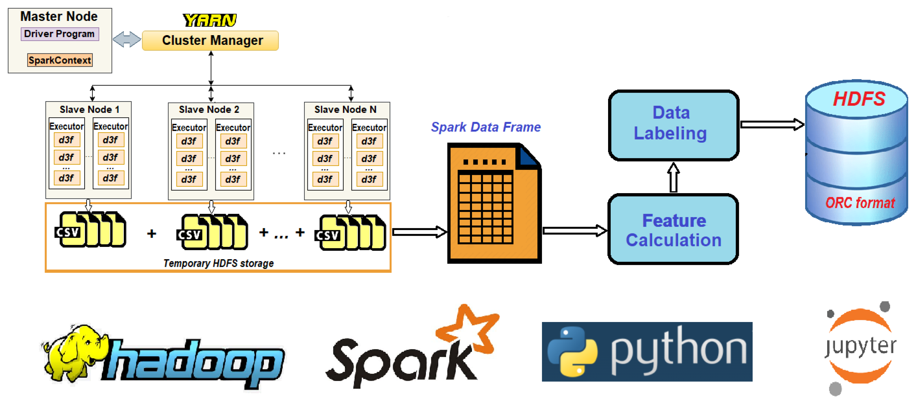
3.2. Big Data Setup for Large-Scale Simulations

In achieving the goals of this study, the authors encountered some challenges related to software engineering and machine learning in a Big Data environment:
  • The implementation of a Big Data setup, allowing mass parallel runs of the legacy d 3 f solver for numerical PDEs;
  • The implementation of the pipelines for collecting, post-processing, and storing large amounts of data from numerical PDEs in the Big Data ecosystem;
  • The implementation of machine learning pipelines for supervised (classification) and unsupervised (dimensionality reduction) models for the studied problem.
Some solutions to these challenges are briefly described below.
A single run of the d 3 f software does not require a special technical environment, and it can be executed on a single workstation. However, we need to execute many runs (thousands, dozens of thousands, or even more) with different parameters and obtain large ensembles of numerical solutions of the governing PDEs (1). These solutions require large amounts of disk space (terabytes or even dozens of terabytes of raw data), CPU, and memory resources, and they take a long time if the d 3 f software is running sequentially on a workstation. It is particularly critical in the case of higher grid levels l 7 , small time steps Δ t , and large ensemble sizes N > 1000 .
For these reasons, the d 3 f software has been ported to a Spark cluster [27]. This allows multiple simulations to run in parallel, saving simulation results to an HDFS (Hadoop file system [44]) in the optimized row columnar (ORC) format with compression [45]. The run time of the d 3 f software in this configuration is dramatically reduced. For example, if the grid level l = 5 , the time step Δ t = 0.2 years, and the simulation time T = 50 years, one run of the d 3 f software takes approx. 5 min. To obtain an ensemble of N = 100,000 solutions, we would need around 347 days if the d 3 f software ran sequentially. This long time for obtaining such a dataset was reduced to approx. 33 h when our Spark setup was used.
This allows us to generate and to analyze very large ensembles of numerical solutions. Our typical run has the following parameters: l = 6 , Δ t = 0.1 years, simulation time T m a x = 50 years (plus some additional steps to obtain steady-state solutions using a different solving schema), and ensemble size N = 10,000 solutions, with a perturbation of the initial conditions. The output of such a run is about 2 Tb of raw data. We used Spark libraries to preprocess our raw data and to solve ML tasks.
From a technical point of view, we implemented the system of parallel runs of legacy d 3 f software that produces comma-separated values (CSV) files with output results. All these files are saved to a given directory in HDFS, together with a file of parameters of each d 3 f run. After completing all d 3 f runs, a Spark job reads all of these files and transforms the data into a Spark dataframe, performs some preprocessing steps, performs labeling of the S1/S2/S3 solutions, calculates features, and finally, saves this data frame to HDFS in ORC format with compression. Our data-processing pipeline is shown in Figure 4. The configuration of our Hadoop/Spark cluster is provided in Table 3.

3.3. Machine Learning

As we already mentioned above, the problem of predicting the steady states of the Elder problem is formulated as a binary (two-class) classification problem. In machine learning, classification is considered an example of supervised learning. In the case of supervised learning, the data are labeled and divided into the following subsets [35,46]:
(i)
A train set with correctly defined labels to fit a model;
(ii)
A validation dataset to estimate the model’s skill while tuning the model’s hyperparameters;
(iii)
A test set to obtain the performance metrics of a trained model.
Finally, the trained model is used to make predictions on new data.
Let X = { X j } , j = 1 , , P be a feature vector, and let Y = { 1 , 2 } be a vector of possible outcomes, i.e., S1 or S2 steady-state solutions. P denotes the number of features (predictors). Each feature is a function of numerical solutions to the Elder problem:
X j = f j ( c ( x , y , t ) )
where c ( x , y , t ) ) = { c i ( t ) } , i = 1 , , N , N is large (see Table 2).
The goal is to predict a steady state with 95% accuracy as early as possible, based on observations from the beginning and up to time t. Many different classification methods [33,34,47] can be used to predict steady states with an acceptable performance. In this study, we use support vector machines (SVMs), random forest (RF), and gradient boosting (GB) classifiers [33,47] implemented in the SciKit-learn package [48], and the Apache Spark MLlib library [49]. This library was also used for PCA, dimensionality reduction, and the complexity analysis of large ensembles of solutions.
The SciKit-learn package in Python [48] was used for preliminary investigations and the design of ML models based on the features precalculated in Spark. Jupyter notebooks [50] were used for interactive data exploration and visualization. All plots were created using the Matplotlib package [51].

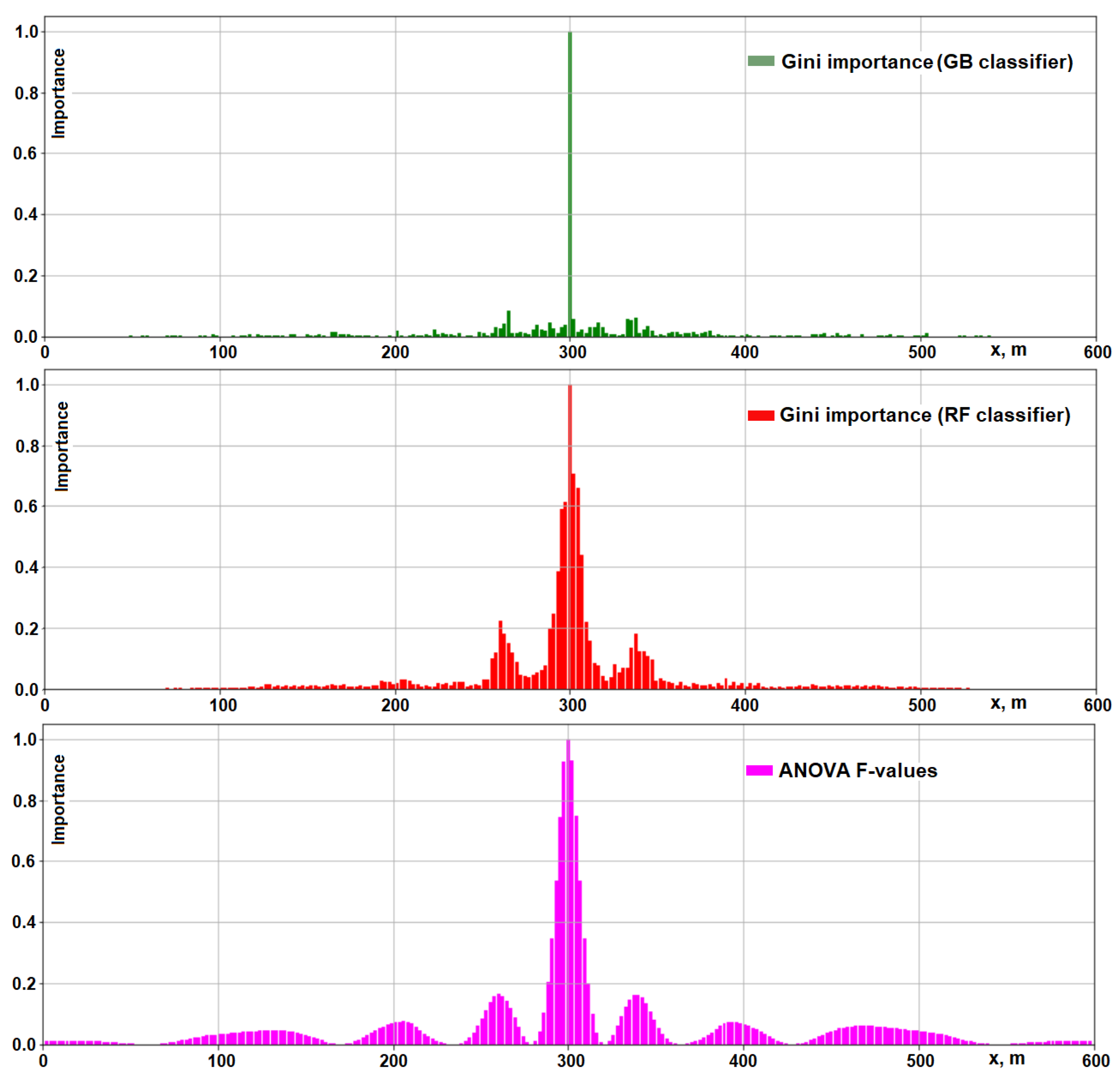
3.4. Feature Engineering

The ML algorithms themselves, the approaches to training, and the validation of ML models are more or less standardized procedures. The important task for an ML algorithm/method is to design a set of features (predictors) that are relevant to the studied process and that can predict an outcome with a given degree of accuracy. This is more critical for the classic ML algorithms used in this paper. For the deep learning models, it is less important, as they are able, in a number of cases, to extract features when fitting a training dataset. There are many approaches, techniques, and tools for feature design or engineering [52]. Some of them can be used for designing predictive models of the Elder problem.
We developed several predictive models for the Elder problem using the classification methods mentioned above. These models are capable of predicting a steady state with acceptable accuracy, and they can be divided into three types, as follows.
  • Fully informed models (Type I);
  • Partially informed models (Type II);
  • Black-box models (Type III).
Type I models are the models based on domain knowledge. This means that we are designing features using all of the possible information about the system studied, including unperturbed transient solutions and steady-state solutions.
Type II. In such models, we design features based on partial knowledge of the system. In our case, we use the knowledge that the presence of fingers characterizes the studied process. Those fingers can be measured using their positions and relative strength, as described in Section 4.3. Thus, we obtain the initial set of features. We then apply one of the feature selection techniques [52] to identify a subset of the most important features. For example, it could be the feature importance based on the Gini impurity [53] implemented in RF and GB classifiers [33], univariate statistical tests [54], or the coefficients of the SVM classifier [47] with the linear kernel. The final model uses k features selected from the initial set. For example, for the solution with grid level l = 6 containing 16,705 values at each time t, we calculate the initial set with 257 features, as described in Section 4.3. Then, we apply one of the feature selection techniques to the initial set and select k = 18 features with the highest importance scores.
Type III models are the models designed using purely data-driven approaches. We do not make any assumptions about the process and we do not use any a priori information for designing features. For example, projections on the k first principal components (PCs) of the original dataset can be used as features in such a classification model.

4. Results and Discussion

In this section, we present some results of our Big Data analysis of the Elder problem based on the approaches and models described above.

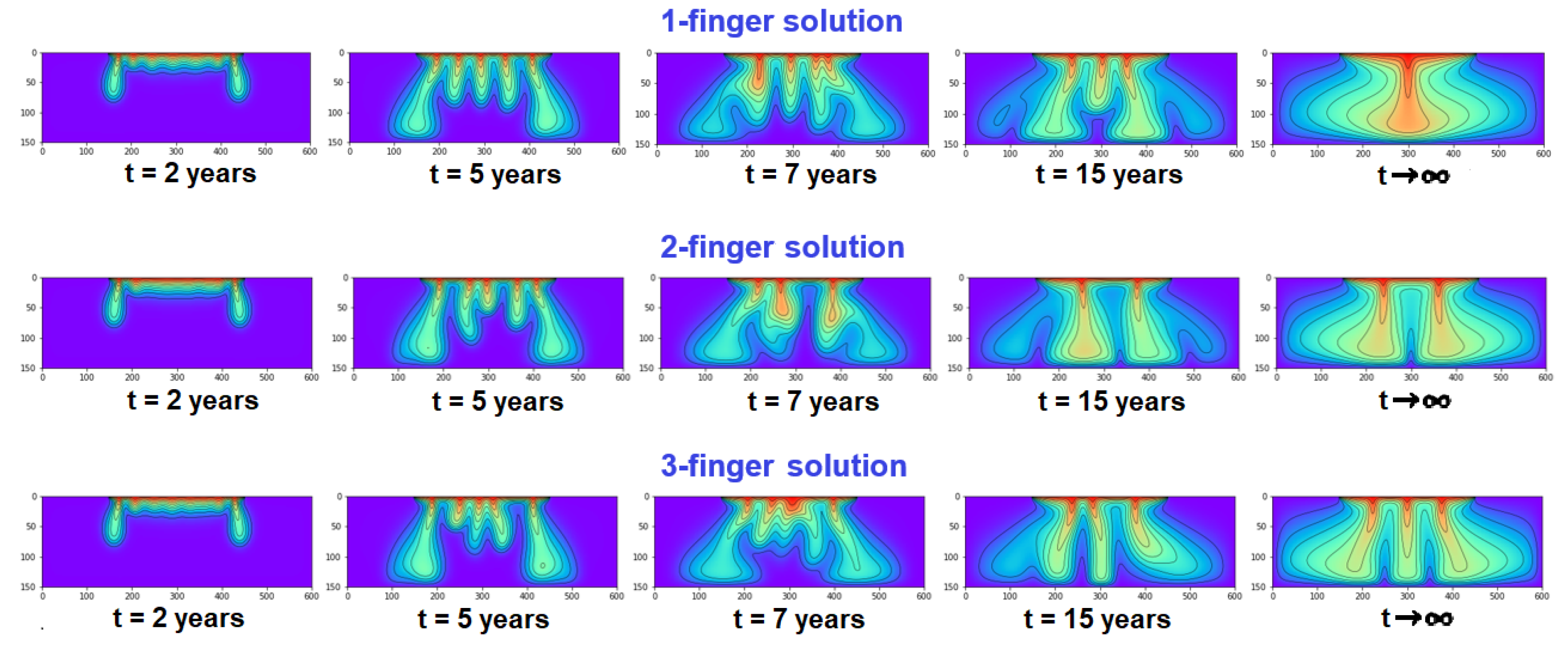
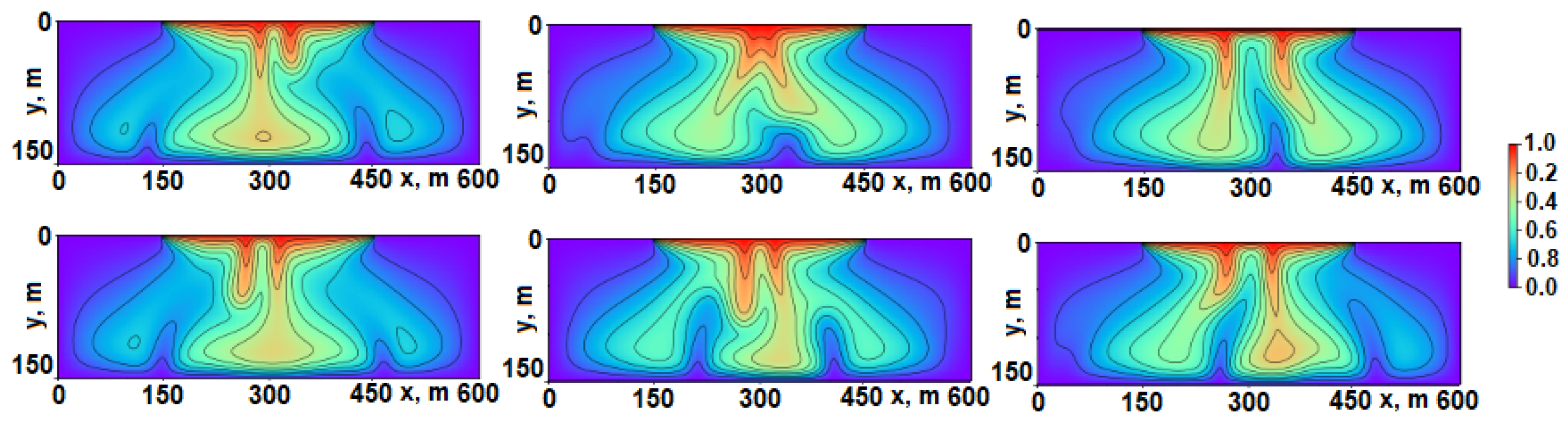
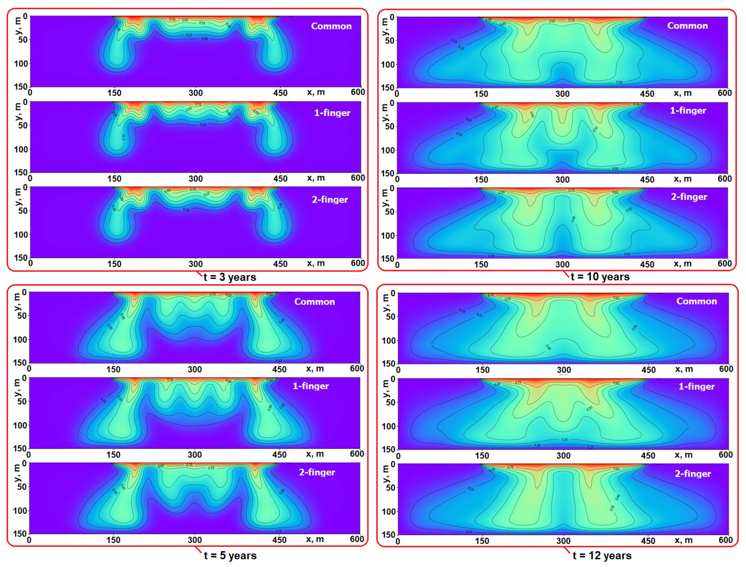
4.1. Unperturbed Solutions

First, aiming to investigate the influences of the different levels l of the grid and time steps Δ t on numerical solutions for the Elder problem, we performed simulations with a wide range of Rayleigh numbers ( R a ) from 0 to 475, with increasing grid levels l = { 6 , 7 , 8 , 9 } and different time steps, such as Δ t = { 0.05 , 0.1 , 0.2 } years, but without any perturbations, that is, the scale of perturbation α = 0 in (6). For the grid with the finest resolution l = 9 (it contains more than 10 6 points), we obtained the following steady-state solutions (Table 4).
We believe that these solutions (Table 4) are the true solutions to the Elder problem for a given R a , and this is our word for the discussion on the right solution to the Elder problem (see Section 2.2). The problem is nonlinear and is highly sensitive to different discretization schemes, time steps, numerical errors, etc. Any of these factors can play the role of perturbations and can cause essential changes in the observed solution dynamics and lead to a steady state that is different from the expected one. Therefore, we consider this situation as a problem that contains uncertainty, and we introduce the conditional probabilities P ^ ( S k | R a ) of the S1/S2/S3 solution, given R a . It is calculated as the ratio of counts, as follows:
P ^ ( S k | R a ) = N S k | R a k = 1 3 N S k | R a ,
where N S k | R a is the number of S k solutions obtained for a given R a , k = 1 , 2 , 3 . Table 5 contains the summary of all our unperturbed simulations, with the estimated probabilities (8) of an S k solution for each given R a .

4.2. Perturbed Solutions

In this and in the following sections, we consider the cases of perturbed simulations. We have generated large ensembles of perturbed solutions for the standard value R a = 400 , perturbing the initial conditions as described above. A typical dataset that is used in this study consists of N = 10,000 solutions (4676 S1 solutions, 5322 S2 solutions, and two S3 solutions) with the time step Δ t = 1 year. For the purpose of predictive modeling, S3 solutions are excluded from the dataset as very rare outcomes. Thus, we have N = 9998 samples that are available at each time t.
Inspecting large ensembles of perturbed solutions to the Elder problem, we observed a number of quite unusual solutions. For example, there are significantly asymmetric solutions (numerically and visually) at time t > 15 years; see Figure 5.
Furthermore, we have obtained steady-state solutions S3 at the standard value R a = 400 of the Rayleigh number. They have a low probability, p 0.0002 . That is, each of our ensembles of solutions contains 1–3 three-finger steady-state solutions.

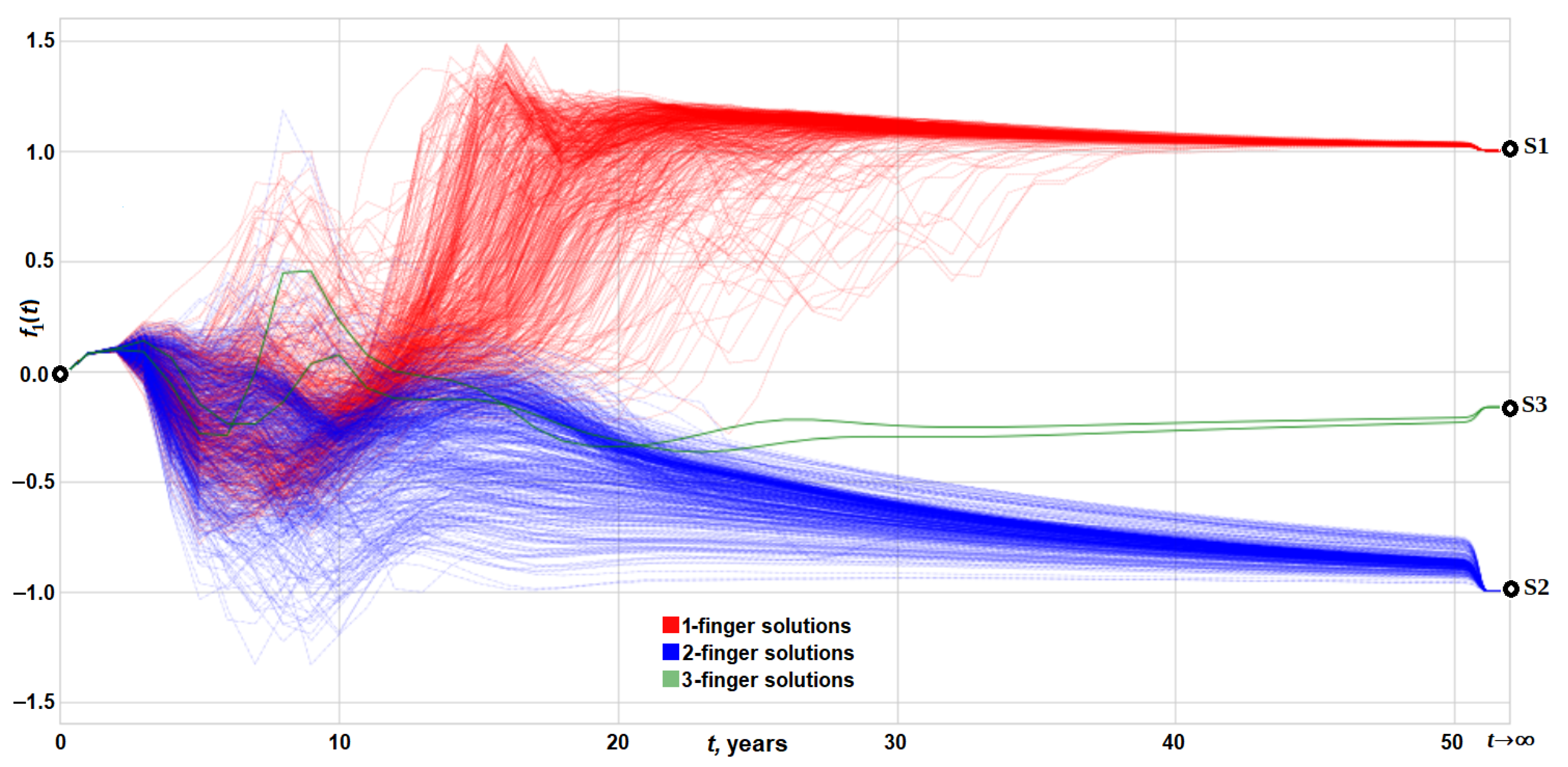
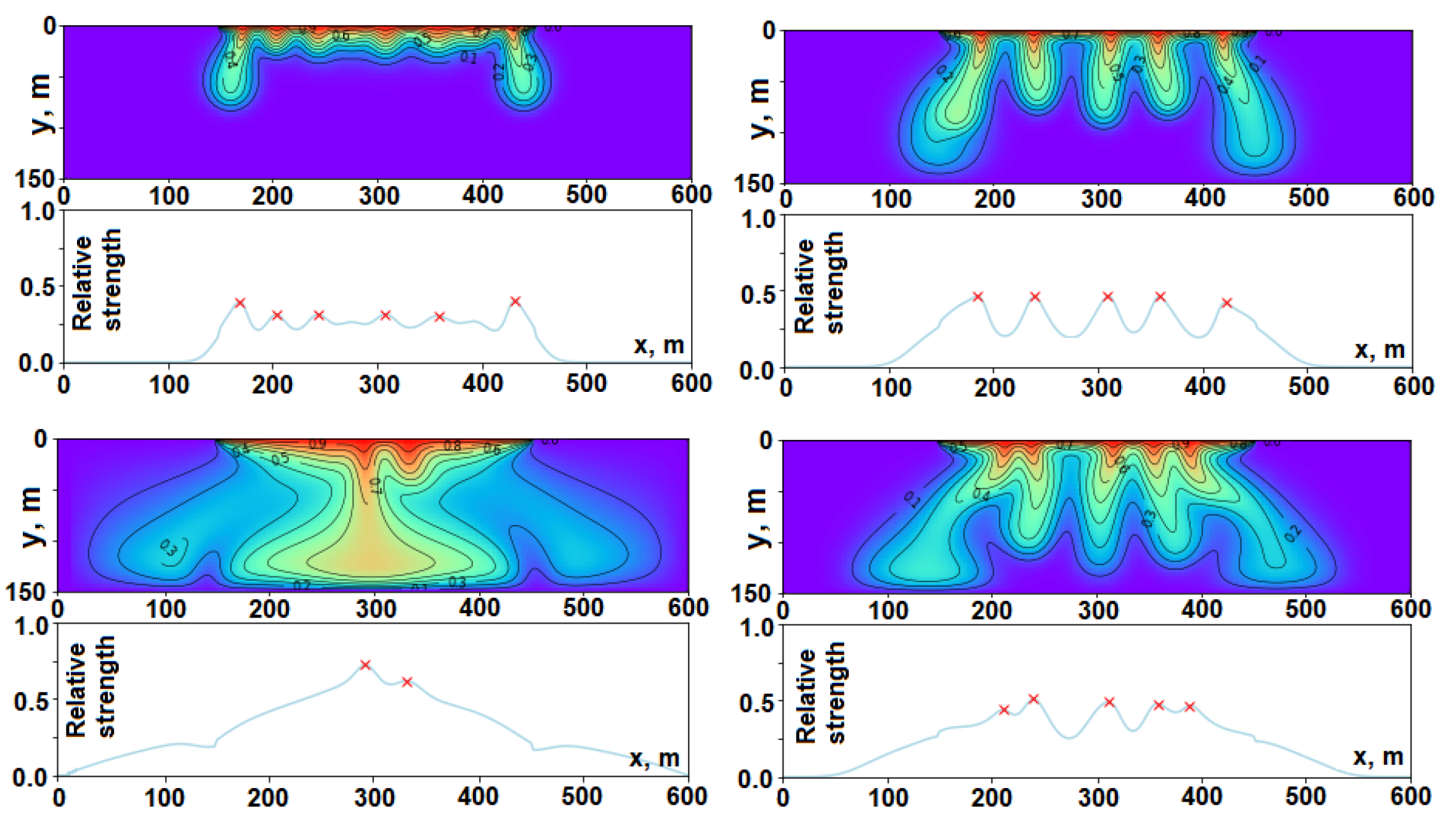
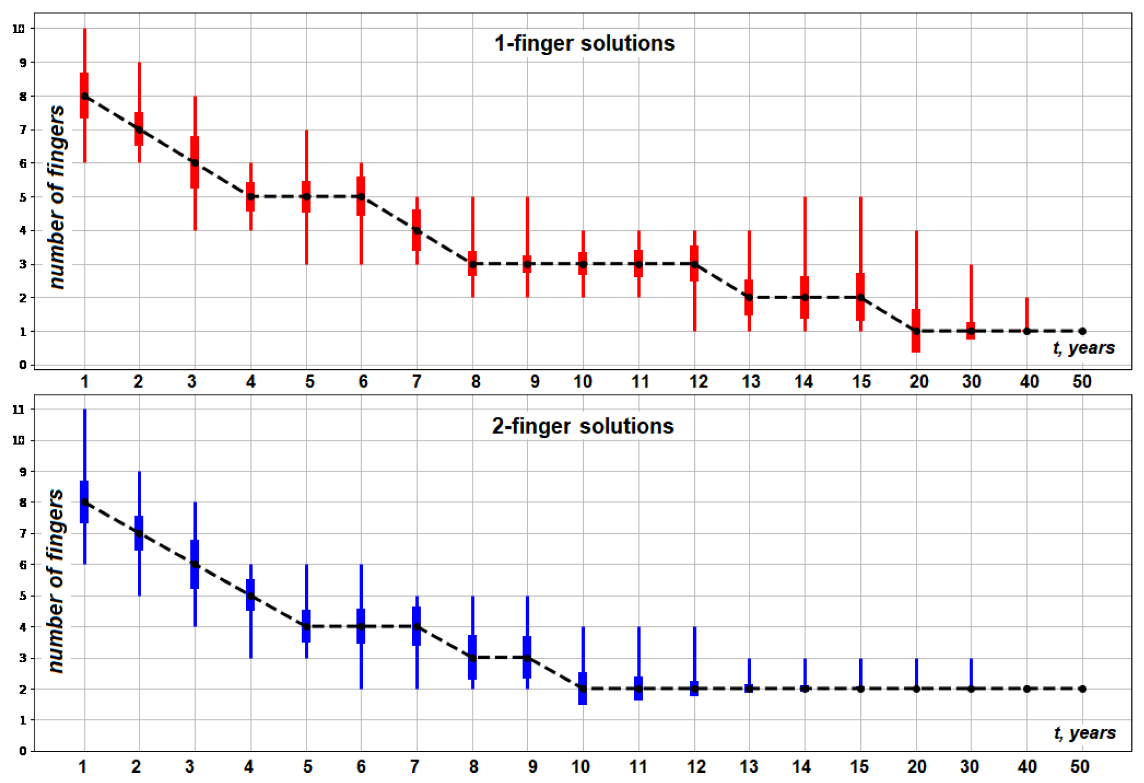
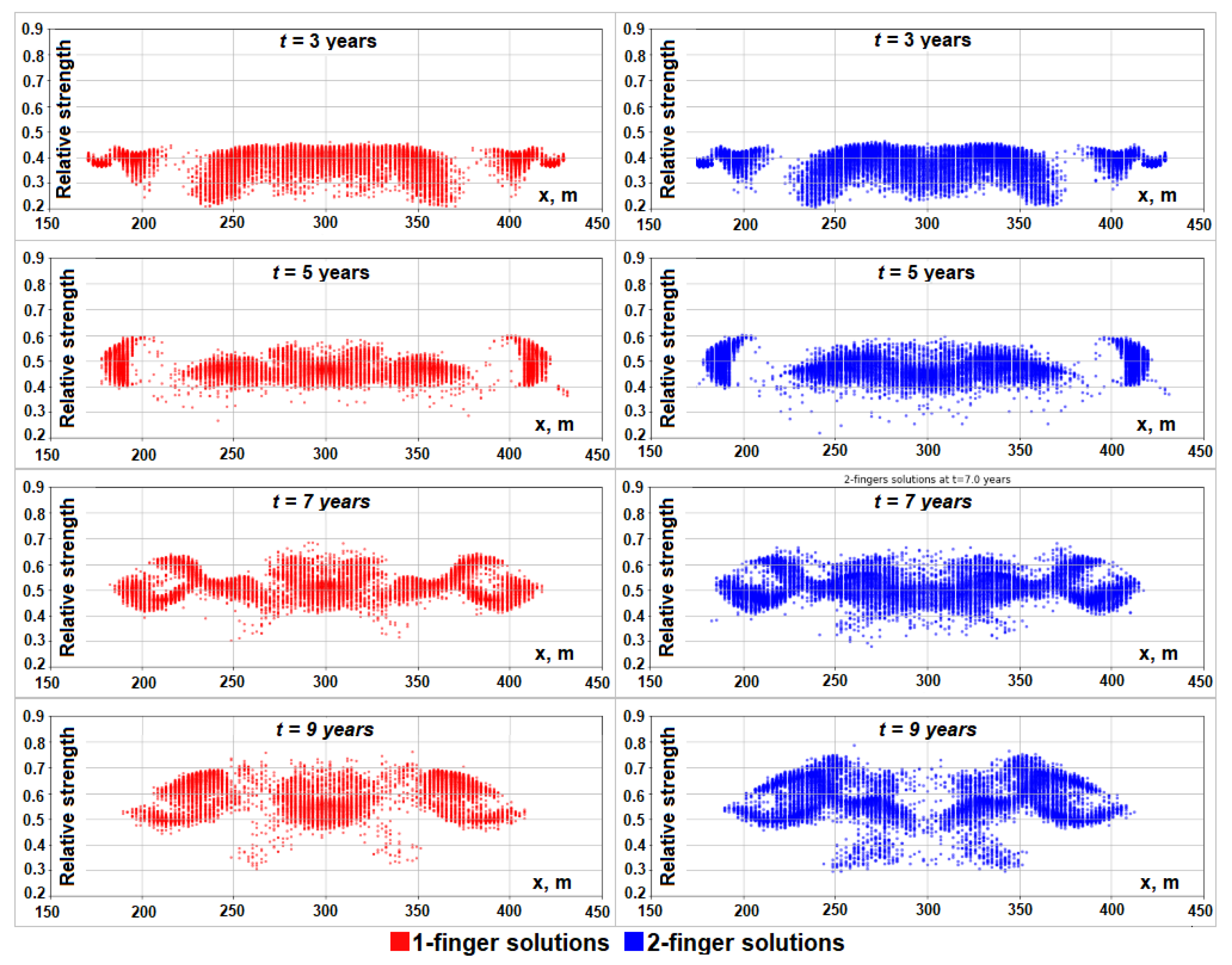
4.3. Identification of Transient Fingers, Their Positions, and Strengths

An important subtask in our study is to calculate the number of fingers in a transient solution of the Elder problem at time t. To achieve this goal, we developed the following approach.
Step 1. Calculate the vertical norm (that is, along the y-axis), L 2 -norm, of the solution for each point x.
Step 2. Divide the values of the L 2 norm by the maximum possible value of the L 2 norm to scale it to the range of [ 0 , 1 ] :
f j = i = 1 n y c i j 2 n y ,
where c i j = c ( x , y ) , i = 1 n y , j = 1 n x .
Step 3. Now, we have a curve (9) with peaks that reflect the position and relative strength of each finger at time t. Then, we just need to find those peaks and calculate the estimated number of fingers n ^ f . It was implemented using the SciPy function find_peaks() [55]. Figure 6 shows four examples of such curves and peaks determined by this algorithm.
Using the abovementioned approach, we calculated the estimated number of fingers for the S1 and S2 solutions at time t = 1 , 2 , , 50 years. As shown in Figure 7, the estimated number of fingers for two-finger solutions decreases faster than for one-finger solutions. It becomes more or less stable at time t = 8–10 years. Probably, this is the time for when it is possible to predict a steady state with acceptable accuracy. We will consider the problem of predicting steady states in Section 4.6 of this paper.

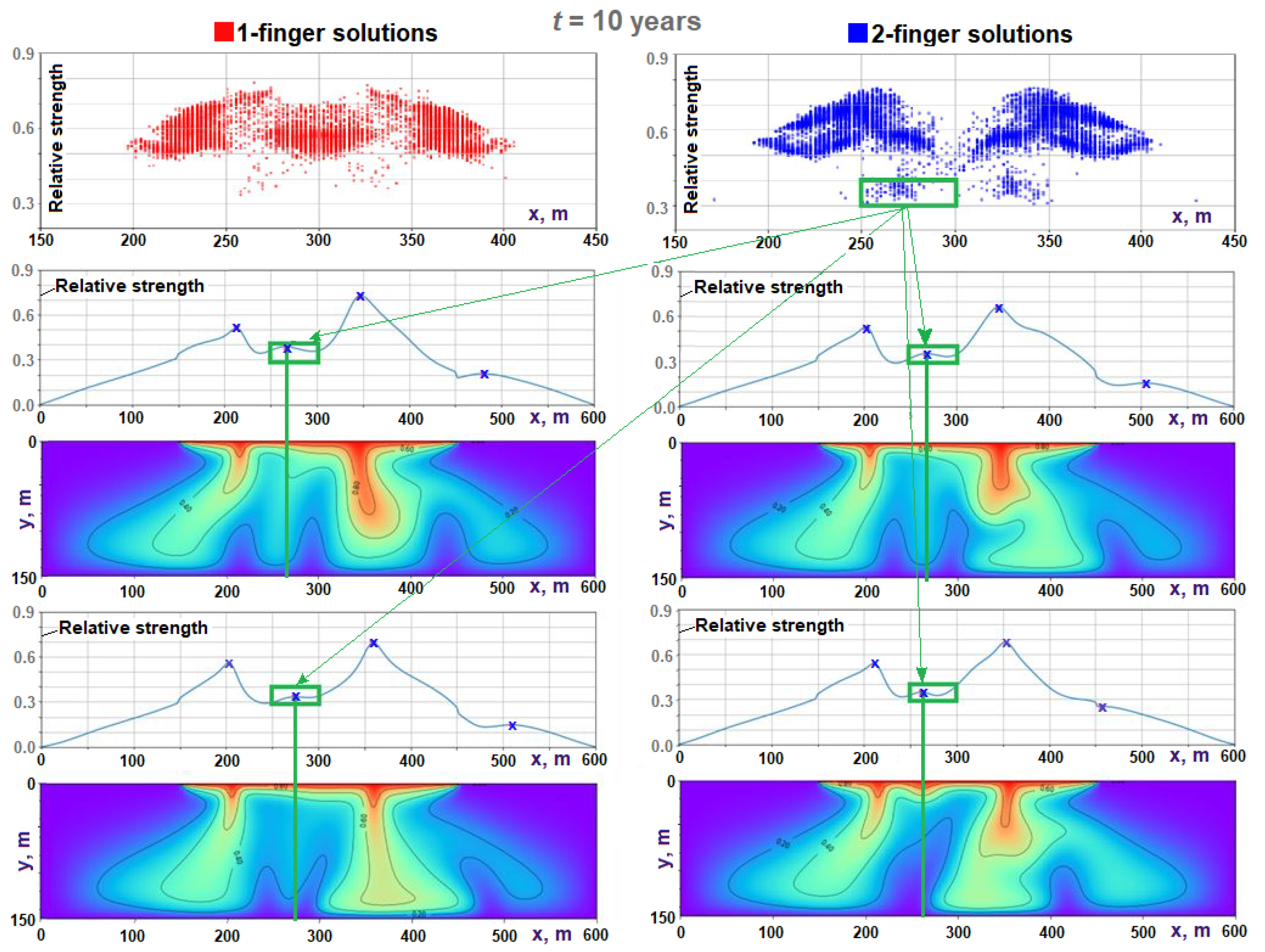
4.4. Interactive Visualization of Transient Solutions and Their Fingers

Based on the approach described in Section 4.3, we developed a tool for the interactive visualization of the fingers (Figure 8). All finger parameters, including the curve (9), are precalculated and saved in HDFS, together with the original solution vectors c ( t ) .
This interactive visualization tool is shown in Figure 8, and works as described below:
  • The positions and strengths of all one- and two-finger solutions in an ensemble at time t are visualized on separate plots.
  • The rectangular selector (in green in Figure 8) is used to specify the selection criteria.
  • Spark executes queries for the solution datasets using given input parameters (that is, the green rectangle in Figure 8), and returns the subset of selected solutions and their curves (9).
This visualization gives us important insights regarding the transient solutions. For example, the points inside the green rectangle in Figure 8 ( t = 10 years, relative strength in the range [ 0.3 , 0.4 ] , x [ 250 , 300 ] m) correspond to the minor fingers in the S2 solutions. These minor fingers disappear at t 10 years.
Another important application of this approach is the possibility of the visual analysis of the dynamical properties of transient solutions at different time steps (i.e., the distribution of fingers in the large ensemble of solutions, considered as a process developing in time). Such distributions for time, t = 3 , 5 , 7 , 9 years, are shown in Figure 9. From this visualization, we can observe a significant difference in the central part of the domain (x = 280–320 m) for S1 solutions, starting from t = 9–10 years. This fact suggests that the most important predictors (features) are likely concentrated in the central part of the rectangular domain.

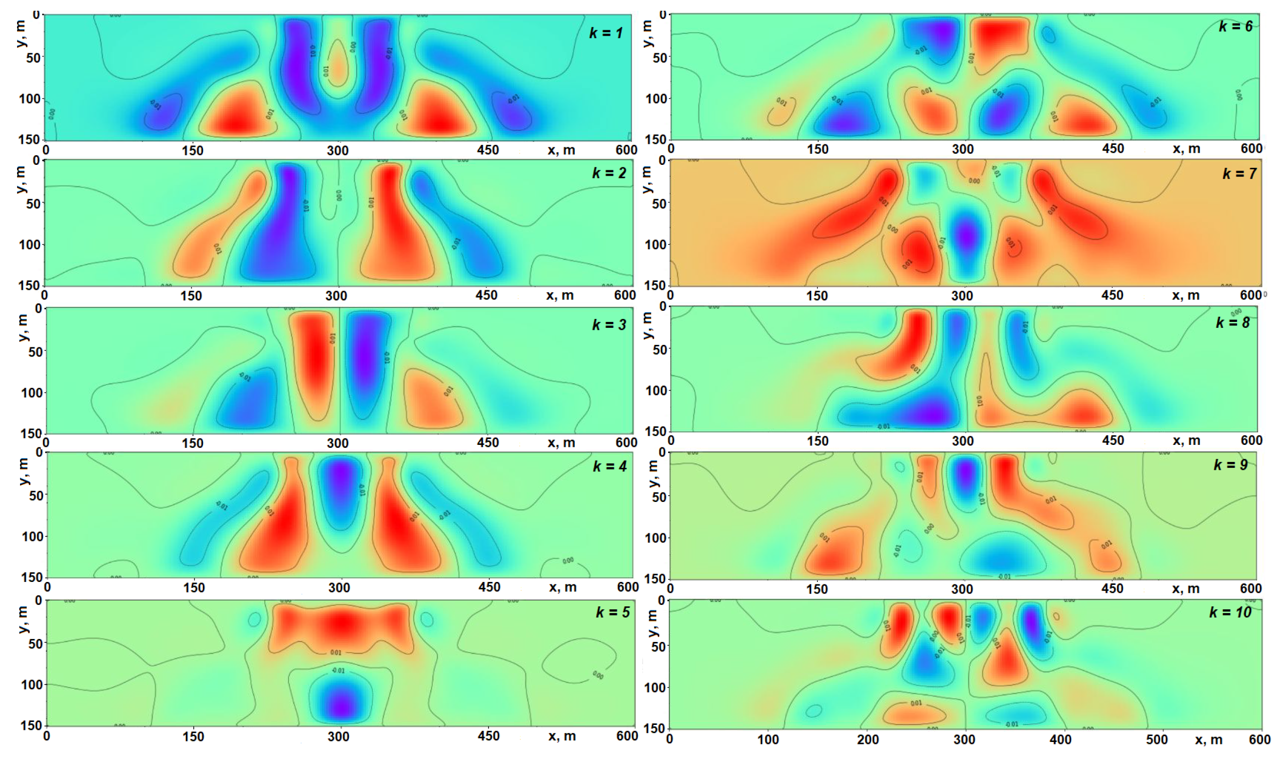
4.5. Complexity Analysis of Transient Solutions

In this section, we analyze the complexity of transient solutions. The high-level description of our analysis is as follows. For each time, t = 1 , 2 , , 50 years, we have the following steps:
  • Create a subset of a dataset ( D S 1 , 2 ) that consists of both one-finger and two-finger solutions at time t.
  • Calculate the SVD of the D S 1 , 2 dataset.
  • Approximate D S 1 , 2 with 95% precision and save the number of principal components k needed for this approximation.
  • Calculate the average solution of the D S 1 , 2 .
  • Create a subset of a dataset D S 1 consisting of only one-finger solutions at time t.
  • Repeat steps 3–4 for the D S 1 dataset, using the set of PCs obtained at step 3.
  • Create a subset of a dataset D S 2 consisting of only two-finger solutions at time t.
  • Repeat steps 3–4 for the D S 2 dataset using the set of PCs obtained at step 3.
Using Spark MLlib, we performed the principal component analysis of the ensemble of N = 10,000 solutions for 1 to 50 years and in the steady state. The results of this complexity analysis are shown in Figure 10. The selected average solutions are presented in Figure 11.
The curves in Figure 10 demonstrate the complexity of transient solutions at different time steps. As we can see from this graph, the complexity of transient solutions starts from the value of 1 at t 1 year, and then rapidly increases and reaches a maximum value of 27 at t = 6–7 years. After that, the complexity starts to decrease and equals to 2 in a steady state. The complexity of two-finger solutions decreases faster than those of one-finger solutions, starting from t = 11 years. It is reasonable to think that the time of highest complexity (t = 6–7 years) determines the limit of predictability, i.e., time T ^ , when it is possible to predict a steady state with acceptable accuracy. Furthermore, the time level around t = 6 was indicated by Diersch and Kolditz [2] as being the most critical for the evolution of the process.
Analyzing the set of average solutions, we noticed that one-finger solutions have a clearly recognizable finger at the center of the domain ( x = 300 m), when the time was t 3 years (see Figure 11). From t 10 years, the average transient solution corresponding to the S1 steady-state solution has three fingers. They merge into a single finger at t > 10 years. We obtained some three-finger solutions (S3) in a steady state. They are rare for standard R a = 400 , e.g., 1–3 S3 solutions in an ensemble of 10,000 solutions. We assume those three fingers observed in the average transient solution are not merging into a single finger in a steady state due to special initial conditions. Thus, we can observe three-finger steady-state solutions (S3).
The first k = 10 principal components at t = 10 years are presented in Figure 12 in order to indicate some symmetric and antisymmetric patterns in these principal components. To explain these patterns, an additional investigation is needed. It will be based, most likely, on even larger ensembles of perturbed solutions.

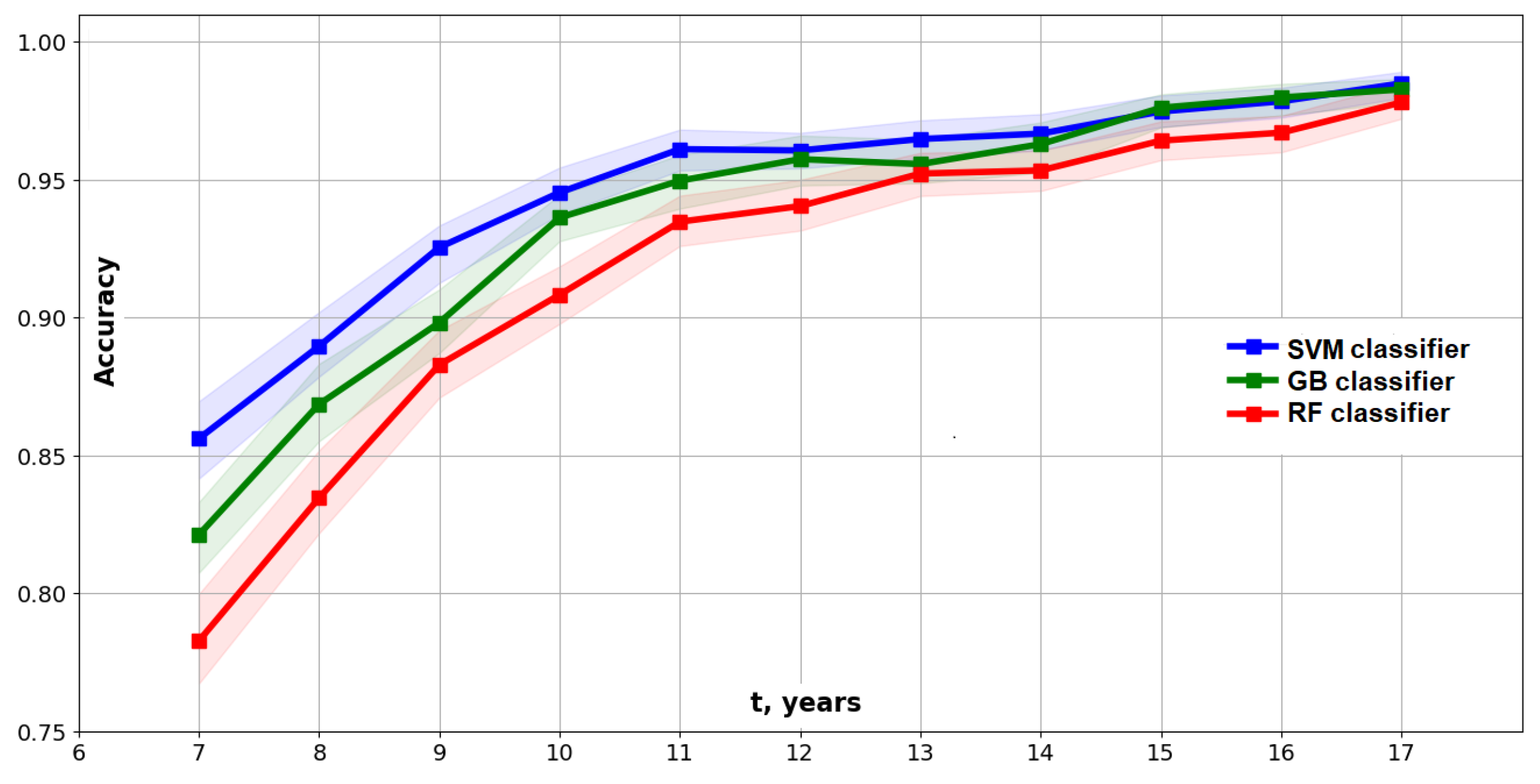
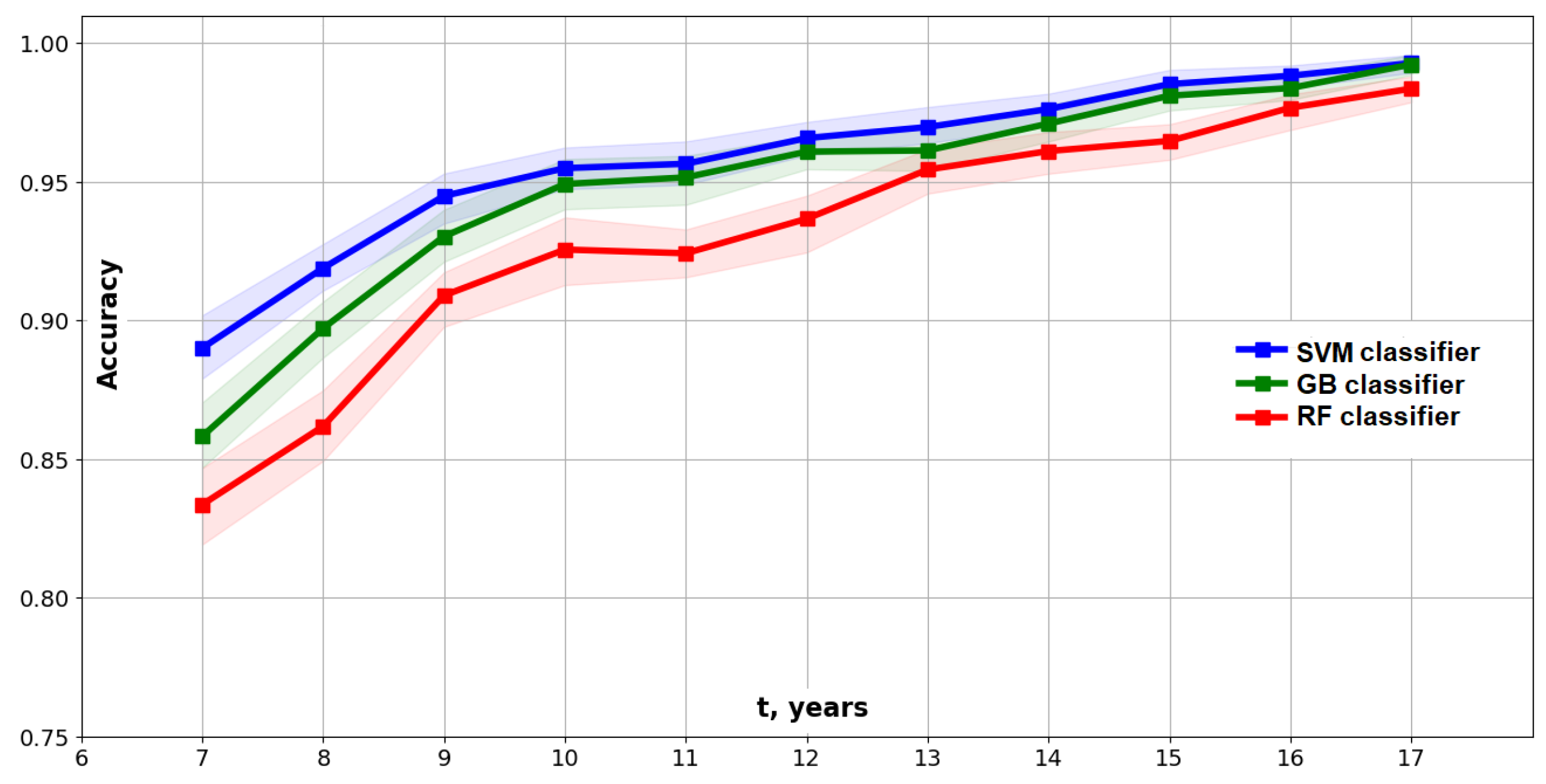
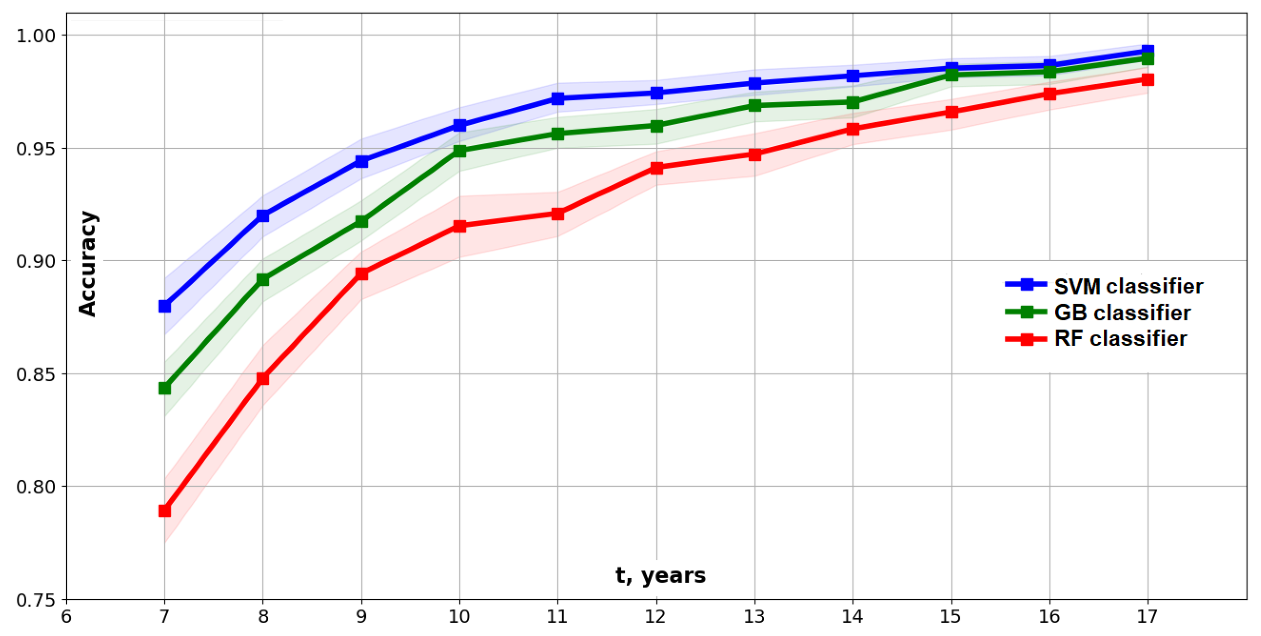
4.6. Predictive Modeling for the Elder Problem

In this section, we present the results of predictive modeling of the Elder problem regarding three types of models, as introduced in Section 3.4. Each of these three models has been implemented with the same number of features X = { f j } , j = 1 , , P , P = 18 to make the three models comparable with each other. Our ML training–testing pipeline is shown in Figure 13 and includes the following steps:
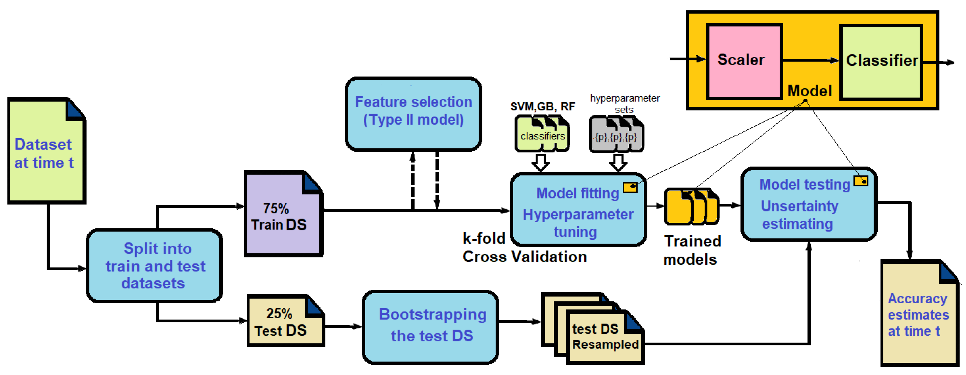
  • Data at time t are queried from HDFS and are transformed into a Pandas data frame.
  • The dataset at time t is randomly divided into training (75%) and testing (25%) datasets.
  • Each model is supposed to be a small internal pipeline (in orange in Figure 13) that consists of a Scaler and a Classifier. Such a solution prevents data leakage in ML models [56].
  • The k-fold cross-validation schema with k = 5 folds is used to search for the best parameters in the hyperparameter spaces. This means that a small internal pipeline is fitted k times on the training datasets, and is evaluated k times on the validation datasets. This block returns the best model and combinations of hyperparameters found on the grid.
  • The features of the training, validation, and testing datasets are scaled using the Standard Scaler, which removes the mean and performs scaling to unit variance.
  • In the case of the Type II model, there is a feature selection step selecting the 18 most important features from the original feature set.
  • Bootstrap is used to create resampled datasets from the test dataset.
  • Finally, we calculate the prediction accuracy and estimate the uncertainty using the resampled datasets for each of the models. Namely, we estimate the mean values and 95% confidence intervals for this accuracy.
On the step of hyperparameter tuning, the following combinations of hyperparameters were used in our classification models. We selected for tuning the hyperparameters that have the most significant influence on the performances of the classifiers.
SMV hyperparameters:
{ k e r n e l = RBF , C , g a m m a } ,
where C is the regularization parameter, that is, the penalty for each misclassified data point, and g a m m a is the kernel coefficient for the radial basis function (RBF) kernel;
RF hyperparameters:
{ n _ e s t i m a t o r s , m a x _ d e p t h , m i n _ s a m p l e s _ s p l i t , m i n _ s a m p l e s _ l e a f } ,
where n _ e s t i m a t o r s is the number of estimators (trees) in the forest, m a x _ d e p t h is the maximum depth of the tree, m i n _ s a m p l e s _ s p l i t is the minimum number of samples required to split an internal node, and m i n _ s a m p l e s _ l e a f is the minimum number of samples at a leaf node;
GB hyperparameters:
{ n _ e s t i m a t o r s , m a x _ d e p t h , l e a r n i n g _ r a t e , m i n _ s a m p l e s _ s p l i t , m i n _ s a m p l e s _ l e a f } ,
where n _ e s t i m a t o r s is the number of boosting stages to perform, m a x _ d e p t h is the maximum number of nodes in the tree, and l e a r n i n g _ r a t e is the parameter controlling the contribution of each model in the ensemble prediction. m i n _ s a m p l e s _ s p l i t and m i n _ s a m p l e s _ l e a f have the same meaning as the RF classifier.
Our Type I model has the following features:
  • The projection of a current solution c ( t ) on the vector
    ν 1 = a 1 c ( S 1 ) + a 2 c ( S 2 ) .
    ν 1 is a linear combination of steady-state solutions c ( S 1 ) and c ( S 2 ) satisfying the conditions below:
    c ( S 1 ) ν 1 = 1 , c ( S 2 ) ν 1 = 1 .
    After inserting (10) into (11) and solving the system of two linear equations, we obtain the coefficients a 1 and a 2 . Originally, the ν 1 vector was designed to automate the labeling of steady-state solutions in large ensembles of solutions. Then, we calculated the projections of all transient solutions on this vector and used them as a feature in the Type I model.
    f 1 ( t ) = c ( t ) ν 1 .
  • The projection of a current solution c ( t ) on vector ν 2 orthogonal to ν 1 is defined as follows:
    f 2 ( t ) = c ( t ) ν 2 ,
    where ν 2 = b 1 c ( S 1 ) + b 2 c ( S 2 ) and ν 1 ν 2 = 0 .
  • The estimated number of fingers (9) (see Section 4.3 for details):
    f 3 ( t ) = n ^ f ( t ) ,
  • Descriptive statistics (mean, standard deviation, and maximum) of a difference between a current perturbed solution c ( t ) and an unperturbed solution c * ( t ) :
    f 4 ( t ) = m e a n ( e ( t ) ) , f 5 ( t ) = s t d d e v ( e ( t ) ) , f 6 ( t ) = m a x ( e ( t ) )
    where e ( t ) = c ( t ) c * ( t ) .
  • The features f j , j = 1 6 described above but taken with a time lag of 1 year:
    f j ( t ) = f j 6 ( t 1 ) , j = 7 12
  • Features f j , j = 1 6 , taken with a time lag of 2 years, are described as follows:
    f j ( t ) = f j 12 ( t 2 ) , j = 13 18
This Type I model can predict a steady state with 95% accuracy at t 10.2 years with the SVM classifier with the RBF kernel (see Figure 14). The GB and RF classifiers demonstrated a lower prediction accuracy for this model (see Table 6).
The Type II model gives us 95% accuracy at t 9.6 years using 18 features selected from the initial 257 features (see Figure 15). Working on the Type II models, we evaluated the following measures of importance for feature selection:
  • The Gini importance in the RF classifier [57].
  • The Gini importance in the GB classifier [58].
  • The F-values, based on the univariate statistical test (ANOVA) and used for univariate feature selection [54].
In Figure 16, the three types of feature importance at t = 9 years are plotted along the x-axis, with scaling to the range [ 0 , 1 ] . This visualization shows us again that the most important features lie in the central part of the domain. The feature selection step in our ML pipeline (see Figure 13) can be developed around any of these three approaches, as each of them gave us quite similar results for the three classifiers mentioned. However, the best accuracy was achieved through the features selected using the GB feature importance. The accuracy of the Type II models is depicted in Figure 15, and the SVM is the best classifier for this model type in our study.
The feature importance along the x-axis in Figure 16 can be interpreted as a statistical measure of the number of fingers occurring in that horizontal region. The fingers are the drivers of the dynamics. The more fingers that occur, the more likely that this region has an important influence in the dynamics of the process, and therefore, the higher the importance is.
In our Type III model, the projections on the first k principal components are used as features in the classification model. The selection of the number k of PCs is based on the complexity analysis of large ensembles of solutions (see Section 4.5). The 95% accuracy level is reached at t 9.3 years using the model with the first k = 18 principal components (Figure 17) as features. SVM with the RBF kernel is again the best classifier.
Overall, our predictive models can predict a steady state with 95% accuracy at t = 9–11 years. PCA is an orthogonal transformation [39], which transforms input data into a set of uncorrelated features. This property of PCA features can explain a slightly better prediction accuracy that is achieved with the Type III model.
Using a linear interpolation of the bootstrapped accuracy data, we estimated the time T ^ , when it is possible to predict a steady state with 95% accuracy for each model type and each classifier (see Table 6).

5. Conclusions

The presented results are focused on analyzing large ensembles of solutions to the Elder problem. This is made possible with our setup based on Big Data tools and data science approaches. We contributed to the discussion on the right solution(s) to the Elder problem, and estimated the conditional probabilities of different steady-state solutions with respect to the value of the Rayleigh number R a .
We developed an approach to identify, visualize, and estimate the positions and strengths of transient fingers. The PCA-based complexity analysis allows us to estimate the complexities of transient solutions, estimate the time of the highest complexity, and reasonably select the number of principal components for supervised ML models at different time steps. We designed and evaluated three possible types of low-order predictive models and their features, and then estimated the prediction accuracy and the time of the 95% predictability of steady states of the Elder problem.
Considering the complexity and the estimated prediction accuracy simultaneously, we can reasonably make the conclusions as follows.
  • A low-order model such as the 18-feature model in this study only has limited capabilities for predicting the full dynamics of the studied system at any given time.
  • At the early time 0 < t < 5 years, the system is nearly unpredictable when using such a low-dimensional (10–20 DoF) model. During this time, we observe quickly growing fingers and the increasing complexity of solutions.
  • At the time 5 < t < 9 years, we observe the highest complexity of solutions and less than 95% predictability.
  • Prediction at the 95% level of accuracy with the 18-feature models becomes possible at the time t > 9 years, when the complexity is significantly decreased. The fingers become more stable and start asymptotically moving to the fingers of a steady-state solution.
  • It might be possible to predict the full dynamics of the Elder problem at time 5 < t < 9 years using models of the order that are higher than 18 features (but that are still low-dimensional models).
These results extend our knowledge of the Elder problem, especially about the properties of large ensembles of perturbed solutions. However, they raise new questions that could be the subject of further studies in the following directions:
  • Investigation of predictability at the transient period 5 < t < 9 years using models of the higher order, as indicated above;
  • More accurate characterizations of transient fingers and their parameters;
  • Nonlinear dimensionality reduction for numerical solutions to the Elder problem;
  • Complexity analysis based on other complexity measures/approaches;
  • Investigation of Deep Learning models for the Elder problem.

Author Contributions

Methodology, supervision, and writing—review and editing, K.J.; software, data, implementation, visualization, and writing—original draft preparation, R.K. All authors have read and agreed to the published version of the manuscript.

Funding

This research was funded by the Research Council of Norway, grant number 259870.

Institutional Review Board Statement

Not applicable.

Informed Consent Statement

Not applicable.

Data Availability Statement

The data related to this study and findings are partially available from the corresponding author upon reasonable request. The raw original datasets are very large, and there are objective limitations on the size of the data provided.

Acknowledgments

The authors appreciate the technical support from the NORCE Norwegian Research Center AS.

Conflicts of Interest

The authors declare no conflict of interest.

Abbreviations

The following abbreviations are used in this paper:
PDEPartial differential equation;
FVMFinite volume method;
FDMFinite difference method;
FEMFinite element method;
R a Rayleigh number;
SUTRA Saturated and/or unsaturated fluid flow, and solute/energy transport;
DMODynamic mesh optimization;
HDFSHadoop file system;
ORCOptimized row columnar;
CSVComma-separated values;
MLMachine learning;
PCPrincipal component;
PCAPrincipal components analysis;
SVDSingular value decomposition;
DoFDegrees of freedom;
SVMSupport vector machines;
RBFRadial basis function;
RFRandom forest;
GBGradient boosting;
ANOVAAnalysis of variation.

References

  1. Elder, J.W. Transient convection in a porous medium. J. Fluid Mech. 1967, 27, 609–623. [Google Scholar] [CrossRef]
  2. Diersch, J.G.; Kolditz, O. Variable-density flow and transport in porous media: Approaches and challenges. Adv. Water Resour. 2002, 25, 899–944. [Google Scholar] [CrossRef]
  3. Voss, C.I.; Souza, W.R. Variable density flow and solute transport simulation of regional aquifers containing a narrow freshwater-saltwater transition zone. Water Resour. 1987, 26, 2097–2106. [Google Scholar] [CrossRef]
  4. Nield, D.A.; Bejan, A. Convection in Porous Media, 4th ed.; Spinger: Berlin/Heidelberg, Germany, 2013; ISBN 978-1-4614-5540-0. [Google Scholar] [CrossRef]
  5. Johannsen, K. On the validity of the Boussinesq approximation for the Elder problem. Comput. Geosci. 2003, 7, 169–182. [Google Scholar] [CrossRef]
  6. Frolkovič, P.; De Schepper, H. Numerical modelling of convection dominated transport coupled with density driven flow in porous media. Adv. Water Resour. 2001, 24, 63–72. [Google Scholar] [CrossRef]
  7. Elder, J.; Simmons, C.T.; Diersch, H.-J.; Frolkovic, P.; Holzbecher, E.; Johannsen, K. The Elder Problem. Fluids 2017, 2, 11. [Google Scholar] [CrossRef] [Green Version]
  8. Simmons, C.T.; Narayan, K.A.; Wooding, R.A. On a test case for density-dependent groundwater flow and solute transport models: The salt lake problem. Water Resour. Res. 1999, 35, 3607–3620. [Google Scholar] [CrossRef]
  9. van Reeuwijk, M.; Mathias, S.A.; Simmons, C.T.; Ward, J.D. Insights from a pseudospectral approach to the Elder problem. Water Resour. Res. 2009, 45, 1–13. [Google Scholar] [CrossRef] [Green Version]
  10. SUTRA: A Model for 2D or 3D Saturated-Unsaturated, Variable-Density Ground-Water Flow with Solute or Energy Transport. Available online: https://www.usgs.gov/software/sutra-model-2d-or-3d-saturated-unsaturated-variable-density-ground-water-flow-solute-or (accessed on 23 December 2022).
  11. Oldenburg, C.; Pruess, K. Dispersive transport dynamics in a strongly coupled groundwater–brine flow system. Water Resour. Res. 1995, 31, 289–302. [Google Scholar] [CrossRef]
  12. Kolditz, O.R.; Ratke, H.-J.; Diersch, W. Coupled groundwater flow and transport: 1. Verification of variable density flow and transport models. Adv. Water Resour. 1998, 21, 7–46. [Google Scholar] [CrossRef]
  13. Prasad, A.; Simmons, C.T. Unstable density-driven flow in heterogeneous porous media: A stochastic study of the Elder “short heater” problem. Water Resour. Res. 2003, 39, 4-1–4-21. [Google Scholar] [CrossRef] [Green Version]
  14. Johannsen, K. The Elder problem—bifurcations and steady state solutions. Dev. Water Sci. 2002, 47, 485–492. [Google Scholar] [CrossRef]
  15. Woods, J.A.; Teubner, M.D.; Simmons, C.T.; Narayan, K. Numerical error in groundwater flow and solute transport simulation. Water Resour. Res. 2003, 39, 1–13. [Google Scholar] [CrossRef] [Green Version]
  16. Thornea, D.T.; Sukopa, M.C. Lattice Boltzmann model for the elder problem. Dev. Water Sci. 2004, 55 Pt 2, 1549–1557. [Google Scholar] [CrossRef]
  17. Musuuza, J.L.; Radu, F.A.; Radu, F.A.; Attinger, S.; Attinger, S. The effect of dispersion on the stability of density-driven flows in saturated homogeneous porous media. Adv. Water Resour. 2011, 34, 417–432. [Google Scholar] [CrossRef]
  18. Ataie-Ashtiani, B.; Simmons, C.T.; Werner, A.D. Influence of Boundary Condition Types on Unstable Density-Dependent Flow. Groundwater 2014, 52, 378–387. [Google Scholar] [CrossRef]
  19. Simmons, C.T.; Elder, J.W. The Elder Problem. Groundwater 2017, 55, 926–930. [Google Scholar] [CrossRef]
  20. Yan, M.; Lu, C.; Yang, J.; Xie, Y.; Luo, J. Impact of Low- or High-Permeability Inclusion on Free Convection in a Porous Medium. Geofluids 2019, 2019, 8609682. [Google Scholar] [CrossRef]
  21. Shafabakhsh, P.; Fahs, M.; Ataie-Ashtiani, B.; Simmons, C.T. Unstable Density-Driven Flow in Fractured Porous Media: The Fractured Elder Problem. Fluids 2019, 4, 168. [Google Scholar] [CrossRef] [Green Version]
  22. Bahlali, M.L.; Salinas, P.; Jackson, M.D. Efficient numerical simulation of density-driven flows: Application to the 2- and 3-D Elder problem. Water Resour. Res. 2022, 58, e2022WR032307. [Google Scholar] [CrossRef]
  23. Xie, Y.; Simmons, C.; Werner, A.; Diersch, J.G. Prediction and uncertainty of free convection phenomena in porous media. Water Resour. Res. 2012, 48, 1944–7973. [Google Scholar] [CrossRef]
  24. Kutz, J.N. Data-Driven Modeling & Scientific Computation: Methods for Complex Systems & Big Data; Oxford University Press: Oxford, UK, 2013; ISBN 978-0-19-966034-6. [Google Scholar]
  25. Brunton, S.; Kutz, J.N. Data-Driven Science and Engineering: Machine Learning, Dynamical Systems, and Control; Oxford University Press: Oxford, UK, 2022; ISBN 9781009089517. [Google Scholar] [CrossRef]
  26. Apache Hadoop. Available online: https://hadoop.apache.org/ (accessed on 23 December 2022).
  27. Apache Spark. Available online: https://spark.apache.org/ (accessed on 23 December 2022).
  28. Fein, E. d3f—Ein Programmpaket zur Modellierung von Dichtegetriebenen Strömungen; GRS: Braunschweig, Germany, 1998; ISBN 3-923875-97-5. [Google Scholar]
  29. Bastian, P.; Birken, K.; Johannsen, K.; Lang, S.; Eckstein, K.; Neuss, N.; Rentz-Reichert, H.; Wieners, C. UG—A Flexible Software Toolbox for Solving Partial Differential Equations. Comput. Vis. Sci. 1997, 1, 27–40. [Google Scholar] [CrossRef] [Green Version]
  30. Ferziger, J.; Perić, M.; Street, R. Computational Methods for Fluid Dynamics, 4th ed.; Springer: Cham, Switzerland, 2020; ISBN 978-3-319-99691-2. [Google Scholar]
  31. ISO Random (The GNU C Library). Available online: https://www.gnu.org/software/libc/manual/html_node/ISO-Random.html#index-rand (accessed on 23 December 2022).
  32. Ajibola, J.; Adam, A.; Ann Muggeridge, A. Gravity Driven Fingering and Mixing During CO2 Sequestration. In Proceedings of the the SPE Asia Pacific Oil & Gas Conference and Exhibition, Perth, Australia, 25–27 October 2016. [Google Scholar] [CrossRef]
  33. Aggarwal, C. (Ed.) Data Classification: Algorithms and Applications; Chapman & Hall/CRC: Boca Raton, FL, USA, 2014; ISBN 1466586745. [Google Scholar]
  34. Bishop, C. Pattern Recognition and Machine Learning; Springer: New York, NY, USA, 2006; ISBN 978-0-387-31073-2. [Google Scholar]
  35. Kuhn, M.; Johnson, K. Applied Predictive Modeling, 2nd ed.; Springer: Berlin/Heidelberg, Germany, 2018; ISBN 978-1461468486. [Google Scholar]
  36. Di Ciccio, T.; Efron, B. Bootstrap confidence intervals. Stat. Sci. 1996, 11, 189–228. [Google Scholar] [CrossRef]
  37. Ho, T.K.; Basu, M. Complexity measures of supervised classification problems. IEEE Trans. Pattern Anal. Mach. Intell. 2002, 24, 289–300. [Google Scholar] [CrossRef] [Green Version]
  38. Baumgartner, R.; Somorjai, R.L. Data complexity assessment in undersampled classification of high-dimensional biomedical data. Pattern Recognit. Lett. 2006, 27, 1383–1389. [Google Scholar] [CrossRef]
  39. Eldén, L. Matrix Methods in Data Mining and Pattern Recognition; Society for Industrial & Applied Mathematics: Philadelphia, PA, USA, 2007; ISBN 978-0-89871-626-9. [Google Scholar]
  40. Dulhare, U.; Ahmad, K.; Bin Ahmad, K.A. (Eds.) Machine Learning and Big Data: Concepts, Algorithms, Tools and Applications.; John Wiley & Sons, Inc.: Hoboken, NJ, USA, 2020; ISBN 9781119654742. [Google Scholar]
  41. Pulliam, T.H.; Zingg, D.W. Fundamentals Algorithms in Computational Fluid Dynamics; Scientific Computation; Springer: Berlin, Germany, 2014. [Google Scholar] [CrossRef]
  42. Chakraverty, S.; Mahato, N.R.; Karunakar, P.; Rao, T.D. Advanced Numerical and Semi-Analytical Methods for Differential Equations; John Wiley & Sons, Inc.: Hoboken, NJ, USA, 2019. [Google Scholar] [CrossRef]
  43. Rapp, B. Microfluidics: Modeling, Mechanics and Mathematics; Elsevier Inc.: Amsterdam, The Netherlands, 2017. [Google Scholar] [CrossRef]
  44. HDFS Architecture Guide. Available online: https://hadoop.apache.org/docs/r1.2.1/hdfs_design.html (accessed on 23 December 2022).
  45. Apache ORC—High-Performance Columnar Storage for Hadoop. Available online: https://orc.apache.org/ (accessed on 23 December 2022).
  46. Brownlee, J. What Is the Difference Between Test and Validation Datasets? 2017. Available online: https://machinelearningmastery.com/difference-test-validation-datasets/ (accessed on 23 December 2022).
  47. Calvetti, D.; Somersalo, E. Mathematics of Data Science: A Computational Approach to Clustering and Classification; Society for Industrial & Applied Mathematics: Philadelphia, PA, USA, 2020; ISBN 9781611976366. [Google Scholar]
  48. Scikit-Learn—Machine Learning in Python. Available online: https://scikit-learn.org/ (accessed on 23 December 2022).
  49. Apache Spark MLlib. Available online: https://spark.apache.org/mllib/ (accessed on 23 December 2022).
  50. Project Jupyter. Available online: https://jupyter.org/ (accessed on 23 December 2022).
  51. Matplotlib: Visualization with Python. Available online: https://matplotlib.org/ (accessed on 23 December 2022).
  52. Duboue, P. The Art of Feature Engineering: Essentials for Machine Learning; Cambridge University Press: Cambridge, UK, 2020. [Google Scholar] [CrossRef]
  53. Hastie, T.; Tibshirani, R.; Friedman, J. The Elements of Statistical Learning: Data Mining, Inference, and Prediction, 2nd ed.; Springer Series in Statistics; Springer: Berlin/Heidelberg, Germany, 2009. [Google Scholar] [CrossRef]
  54. Univariate Feature Selection—Scikit-Learn 1.2.0 Documentation. Available online: https://scikit-learn.org/stable/modules/feature_selection.html#univariate-feature-selection (accessed on 23 December 2022).
  55. Scipy.Signal.Find_PEAKS—SciPy v1.9.1 Manual. Available online: https://docs.scipy.org/doc/scipy/reference/generated/scipy.signal.find_peaks.html (accessed on 23 December 2022).
  56. Tingle, M. Preventing Data Leakage in Your Machine Learning Model. Available online: https://towardsdatascience.com/preventing-data-leakage-in-your-machine-learning-model-9ae54b3cd1fb (accessed on 26 February 2023).
  57. Random Forest Classifier—Scikit-Learn 1.2.0 Documentation. Available online: https://scikit-learn.org/stable/modules/generated/sklearn.ensemble.RandomForestClassifier.html#sklearn.ensemble.RandomForestClassifier.feature_importances_ (accessed on 23 December 2022).
  58. Gradient Boosting Classifier—Scikit-Learn 1.2.0 Documentation. Available online: https://scikit-learn.org/stable/modules/generated/sklearn.ensemble.GradientBoostingClassifier.html#sklearn.ensemble.GradientBoostingClassifier.feature_importances_ (accessed on 23 December 2022).
Figure 1. The Elder problem: domain, boundary conditions, and the l = 2 grid.
Bdcc 07 00052 g001
Figure 2. Development in time of the Elder problem for 1-, 2-, and 3-finger solutions.
Bdcc 07 00052 g002
Figure 3. The behavior of the feature (12) in time for the ensemble of N = 10,000 solutions.
Bdcc 07 00052 g003
Figure 4. The data-processing pipeline.
Bdcc 07 00052 g004
Figure 5. Asymmetric solutions at t > 15 years.
Bdcc 07 00052 g005
Figure 6. Examples of the curve (9) and the peaks (the x markers in red) corresponding to the solution fingers.
Bdcc 07 00052 g006
Figure 7. Estimated number of fingers (median, min, max, and stddev) for 1- and 2-finger solutions.
Bdcc 07 00052 g007
Figure 8. Visualization of the fingers of 2-finger solutions for a given subset of positions and strengths (the area inside the green rectangle). The x markers in blue indicate the peaks of the curve (9).
Bdcc 07 00052 g008
Figure 9. Distributions of fingers in the ensemble of N = 10,000 solutions at t = 3 , 5 , 7 , 9 years.
Bdcc 07 00052 g009
Figure 10. The number of principal components needed for the approximation with 95% precision.
Bdcc 07 00052 g010
Figure 11. Average solutions at t = 3 , 5 , 10 , 12 years.
Bdcc 07 00052 g011
Figure 12. The first 10 principal components at t = 10 years.
Bdcc 07 00052 g012
Figure 13. Machine learning pipeline.
Bdcc 07 00052 g013
Figure 14. Accuracy of the Type I model: mean values and 95% confidence intervals.
Bdcc 07 00052 g014
Figure 15. Accuracy of the Type II model: mean values and 95% confidence intervals.
Bdcc 07 00052 g015
Figure 16. Feature importance at t = 9 years for the Type II models (scaled to the range [0, 1]).
Bdcc 07 00052 g016
Figure 17. Accuracy of the Type III model: mean values and 95% confidence intervals.
Bdcc 07 00052 g017
Table 1. Parameters of the Elder problem.
NameSymbolValueUnit
Porosityn0.1-
Molecular diffusion coefficient D m 3.565 × 10 6 m 2 · s 1
Viscosity μ 0.001kg· m 1
PermeabilityK 4.845 × 10 13 m 2
Max. salt mass fraction ω m a x 20%-
Min. density ρ m i n 1000.0kg· m 3
Max. density ρ m a x 1200.0kg· m 3
Gravityg9.81 s 2
Table 2. Number of nodes at the grid level l.
l123456789
n x 359173365129257513
n y 917336512925751310252049
N27852971105425716,70566,177263,4251,051,137
Table 3. Hadoop cluster configuration.
ParameterValue
Number of nodes10
CPU type×86_64, the mix of Intel and AMD CPUs
Total cores available208 (416 threads)
Total memory (RAM) available1792 GB
RAM per nodefrom 128 to 256 GB
HDFS storage available192 TB
Cluster managerYARN
Table 4. Steady-state solutions obtained for different R a on the grid l = 9 .
Ra 0255075100125150175200225
SolutionS1S1S1S1S2S2S2S1S2S2
Ra 250275300325350375400425450475
SolutionS1S3S3S2S2S2S1S1S1S1
Table 5. Conditional probabilities P ^ ( S k | R a ) of S k solutions, k = { 1 , 2 , 3 } .
Sk | Ra 0255075100125150175200225
S 1 1.001.001.000.830.000.000.480.870.000.00
S 2 0.000.000.000.171.001.000.520.001.001.00
S 3 0.000.000.000.000.000.000.000.130.000.00
Sk | Ra 250275300325350375400425450475
S 1 0.700.000.000.130.000.000.520.710.860.65
S 2 0.300.220.040.570.870.860.330.290.140.35
S 3 0.000.780.960.300.130.140.140.000.000.00
Table 6. Estimated time T ^ of 95% predictability in years (mean values and 95% confidence intervals).
Model TypeSVM ClassifierGB ClassifierRF Classifier
Type I 10.21 9.73 , 10.76 11.09 10.44 , 13.09 13.13 12.17 , 14.32
Type II 9.62 8.94 , 11.05 10.57 9.75 , 11.52 12.75 12.42 , 13.23
Type III 9.32 8.94 , 9.74 10.30 9.83 , 11.11 13.31 12.71 , 14.26
Disclaimer/Publisher’s Note: The statements, opinions and data contained in all publications are solely those of the individual author(s) and contributor(s) and not of MDPI and/or the editor(s). MDPI and/or the editor(s) disclaim responsibility for any injury to people or property resulting from any ideas, methods, instructions or products referred to in the content.

