

Classification of Microbiome Data from Type 2 Diabetes Mellitus Individuals with Deep Learning Image Recognition
 , , ,
, , ,
Abstract
:1. Introduction
2. Materials and Methods
2.1. Sample Preparation and NGS Data Processing
2.2. Dataset and Study Group
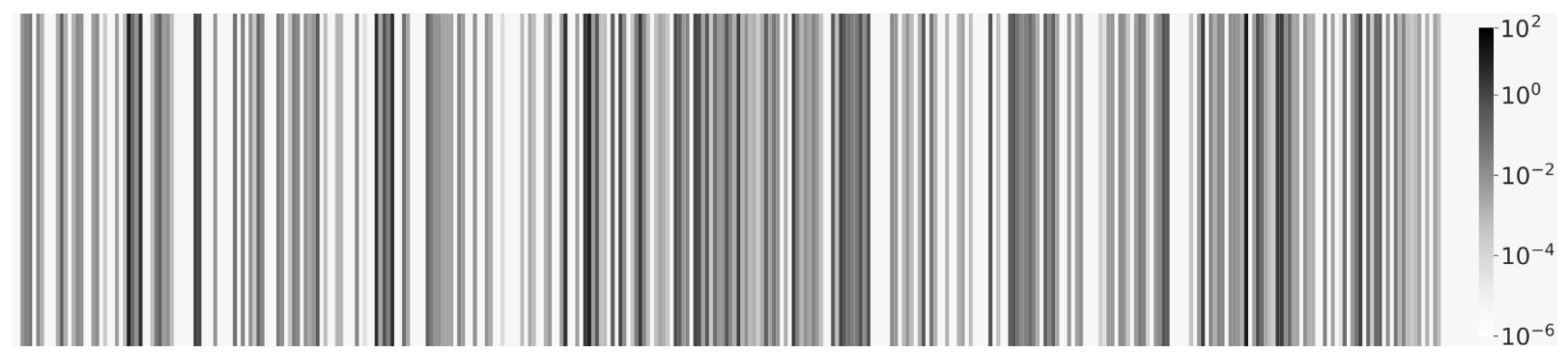
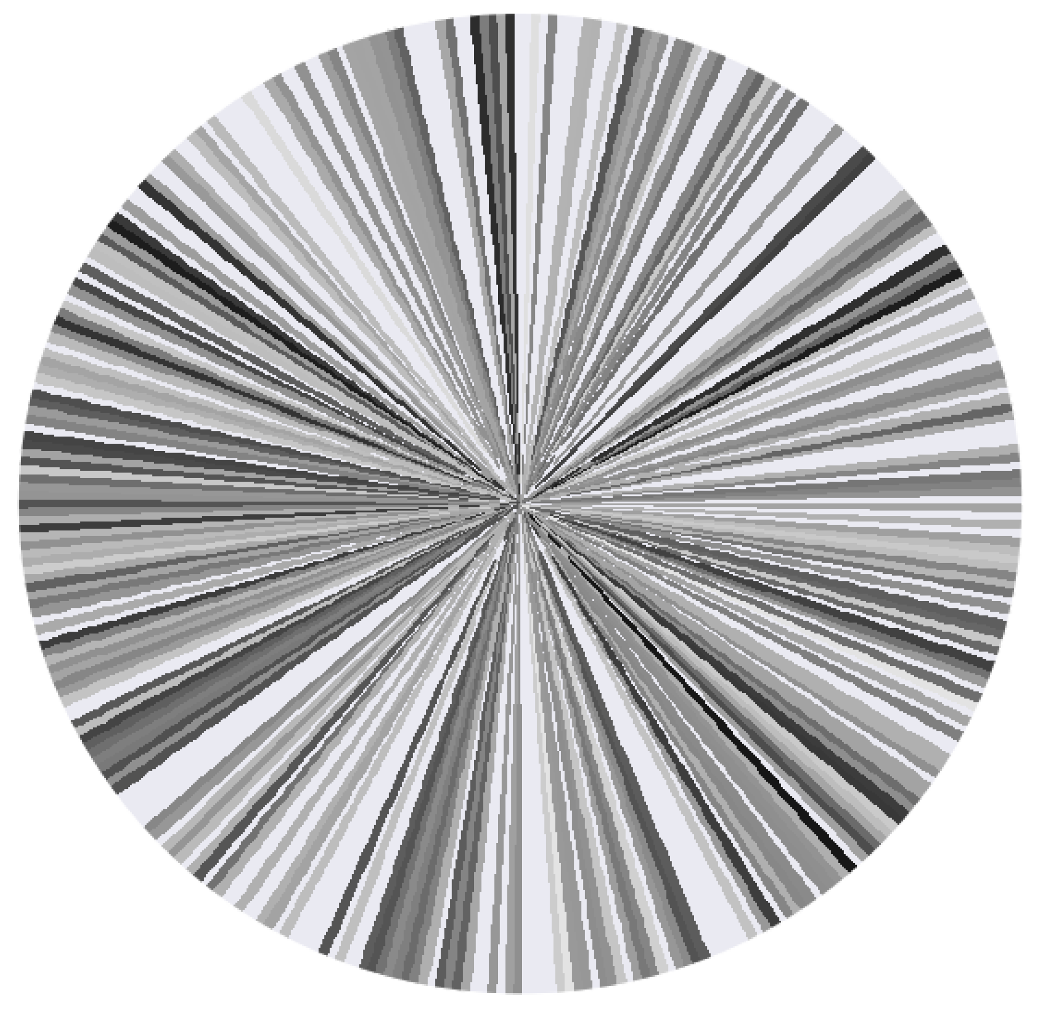
2.3. Visualization Methods
2.4. ML/DL Algorithms and Training
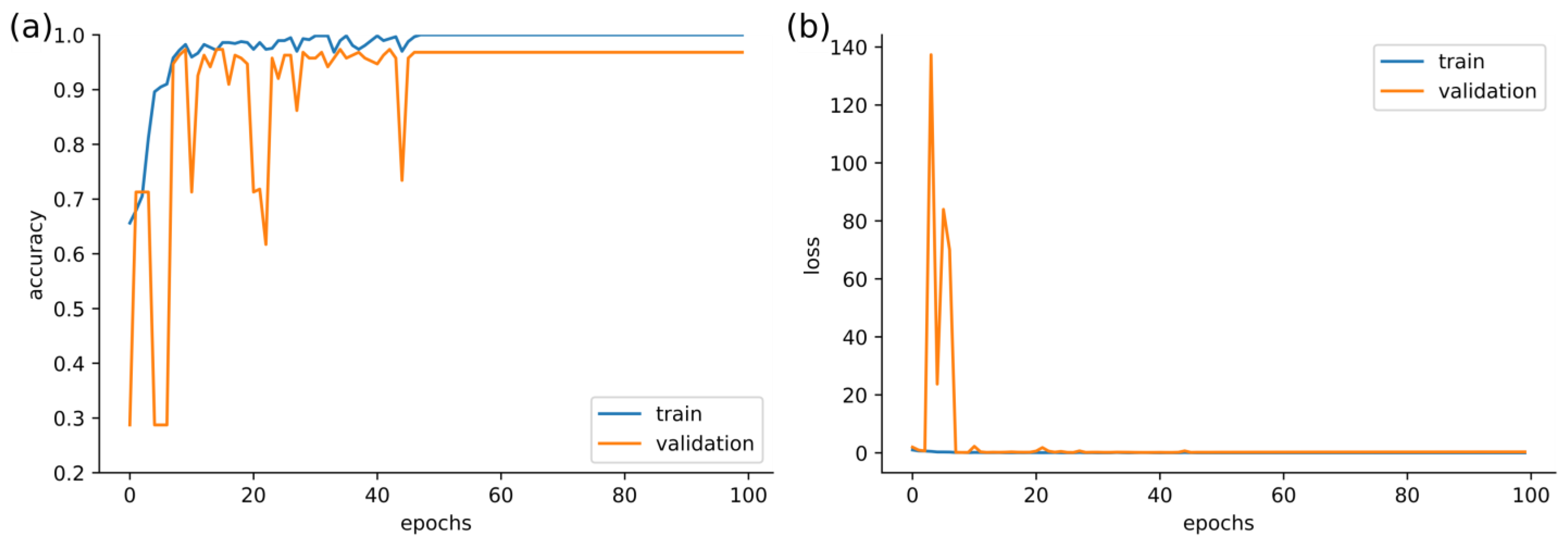
3. Results
4. Discussion and Conclusions
Author Contributions
Funding
Institutional Review Board Statement
Informed Consent Statement
Data Availability Statement
Acknowledgments
Conflicts of Interest
References
- Fan, Y.; Pedersen, O. Gut Microbiota in Human Metabolic Health and Disease. Nat. Rev. Microbiol. 2021, 19, 55–71. [Google Scholar] [CrossRef]
- Akimbekov, N.S.; Digel, I.; Sherelkhan, D.K.; Lutfor, A.B.; Razzaque, M.S. Vitamin D and the Host-Gut Microbiome: A Brief Overview. Acta Histochem. Cytochem. 2020, 53, 33–42. [Google Scholar] [CrossRef] [PubMed]
- Davis, C.D. The Gut Microbiome and Its Role in Obesity. Nutr. Today 2016, 51, 167. [Google Scholar] [CrossRef] [PubMed] [Green Version]
- Gevers, D.; Kugathasan, S.; Denson, L.A.; Vázquez-Baeza, Y.; Van Treuren, W.; Ren, B.; Schwager, E.; Knights, D.; Song, S.J.; Yassour, M. The Treatment-Naive Microbiome in New-Onset Crohn’s Disease. Cell Host Microbe 2014, 15, 382–392. [Google Scholar] [CrossRef] [PubMed] [Green Version]
- Sears, C.L.; Garrett, W.S. Microbes, Microbiota, and Colon Cancer. Cell Host Microbe 2014, 15, 317–328. [Google Scholar] [CrossRef] [Green Version]
- Xu, H.; Liu, M.; Cao, J.; Li, X.; Fan, D.; Xia, Y.; Lu, X.; Li, J.; Ju, D.; Zhao, H. The Dynamic Interplay between the Gut Microbiota and Autoimmune Diseases. J. Immunol. Res. 2019, 2019, 351–364. [Google Scholar] [CrossRef] [Green Version]
- Zhang, H.; Chen, Y.; Wang, Z.; Xie, G.; Liu, M.; Yuan, B.; Chai, H.; Wang, W.; Cheng, P. Implications of Gut Microbiota in Neurodegenerative Diseases. Front. Immunol. 2022, 13, 325. [Google Scholar] [CrossRef] [PubMed]
- Hasan, N.; Yang, H. Factors Affecting the Composition of the Gut Microbiota, and Its Modulation. PeerJ 2019, 7, e7502. [Google Scholar] [CrossRef] [PubMed] [Green Version]
- Loncar-Turukalo, T.; Claesson, M.J.; Bertelsen, R.J.; Zomer, A.; D’Elia, D. Towards the Optimisation and Standardisation of Machine Learning Techniques for Human Microbiome Research: The ML4Microbiome COST Action (CA 18131). EMBnet J. 2020, 26, 997. [Google Scholar] [CrossRef]
- Bansal, N. Prediabetes Diagnosis and Treatment: A Review. World J. Diabetes 2015, 6, 296. [Google Scholar] [CrossRef]
- Wukich, D.K.; Raspovic, K.M.; Suder, N.C. Patients with Diabetic Foot Disease Fear Major Lower-Extremity Amputation More than Death. Foot Ankle Spec. 2018, 11, 17–21. [Google Scholar] [CrossRef] [Green Version]
- Wensel, C.R.; Pluznick, J.L.; Salzberg, S.L.; Sears, C.L. Next-Generation Sequencing: Insights to Advance Clinical Investigations of the Microbiome. J. Clin. Investig. 2022, 132, e154944. [Google Scholar] [CrossRef]
- Douglas, G.M.; Maffei, V.J.; Zaneveld, J.R.; Yurgel, S.N.; Brown, J.R.; Taylor, C.M.; Huttenhower, C.; Langille, M.G. PICRUSt2 for Prediction of Metagenome Functions. Nat. Biotechnol. 2020, 38, 685–688. [Google Scholar] [CrossRef]
- Moreno-Indias, I.; Lahti, L.; Nedyalkova, M.; Elbere, I.; Roshchupkin, G.; Adilovic, M.; Aydemir, O.; Bakir-Gungor, B.; Santa Pau, E.C.; D’Elia, D. Statistical and Machine Learning Techniques in Human Microbiome Studies: Contemporary Challenges and Solutions. Front. Microbiol. 2021, 12, 277. [Google Scholar] [CrossRef]
- Shwartz-Ziv, R.; Armon, A. Tabular Data: Deep Learning Is Not All You Need. Inf. Fusion 2022, 81, 84–90. [Google Scholar] [CrossRef]
- Namkung, J. Machine Learning Methods for Microbiome Studies. J. Microbiol. 2020, 58, 206–216. [Google Scholar] [CrossRef]
- Sharma, D.; Paterson, A.D.; Xu, W. TaxoNN: Ensemble of Neural Networks on Stratified Microbiome Data for Disease Prediction. Bioinformatics 2020, 36, 4544–4550. [Google Scholar] [CrossRef]
- Reitmeier, S.; Kiessling, S.; Clavel, T.; List, M.; Almeida, E.L.; Ghosh, T.S.; Neuhaus, K.; Grallert, H.; Linseisen, J.; Skurk, T. Arrhythmic Gut Microbiome Signatures Predict Risk of Type 2 Diabetes. Cell Host Microbe 2020, 28, 258–272. [Google Scholar] [CrossRef]
- Hernández Medina, R.; Kutuzova, S.; Nielsen, K.N.; Johansen, J.; Hansen, L.H.; Nielsen, M.; Rasmussen, S. Machine Learning and Deep Learning Applications in Microbiome Research. ISME Commun. 2022, 2, 98. [Google Scholar] [CrossRef]
- Mulenga, M.; Kareem, S.A.; Sabri, A.Q.M.; Seera, M.; Govind, S.; Samudi, C.; Mohamad, S.B. Feature Extension of Gut Microbiome Data for Deep Neural Network-Based Colorectal Cancer Classification. IEEE Access 2021, 9, 23565–23578. [Google Scholar] [CrossRef]
- He, K.; Zhang, X.; Ren, S.; Sun, J. Deep Residual Learning for Image Recognition. In Proceedings of the IEEE Conference on Computer Vision and Pattern Recognition, Las Vegas, NV, USA, 27–30 June 2016; pp. 770–778. [Google Scholar]
- Sarwinda, D.; Paradisa, R.H.; Bustamam, A.; Anggia, P. Deep Learning in Image Classification Using Residual Network (ResNet) Variants for Detection of Colorectal Cancer. Procedia Comput. Sci. 2021, 179, 423–431. [Google Scholar] [CrossRef]
- O’Mahony, N.; Campbell, S.; Carvalho, A.; Harapanahalli, S.; Hernandez, G.V.; Krpalkova, L.; Riordan, D.; Walsh, J. Deep Learning vs. Traditional Computer Vision. In Advances in Computer Vision, Proceedings of the 2019 Computer Vision Conference (CVC), Las Vegas, NV, USA, 2–3 May 2019; Springer: Cham, Switzerland, 2019; pp. 128–144. [Google Scholar]
- Wang, W.; Yang, Y.; Wang, X.; Wang, W.; Li, J. Development of Convolutional Neural Network and Its Application in Image Classification: A Survey. Opt. Eng. 2019, 58, 040901. [Google Scholar] [CrossRef] [Green Version]
- Reiman, D.; Metwally, A.; Dai, Y. Using Convolutional Neural Networks to Explore the Microbiome. In Proceedings of the 2017 39th Annual International Conference of the IEEE Engineering in Medicine and Biology Society (EMBC), Jeju Island, Republic of Korea, 11–15 July 2017; IEEE: New York, NY, USA, 2017; pp. 4269–4272. [Google Scholar]
- Reiman, D.; Farhat, A.M.; Dai, Y. Predicting Host Phenotype Based on Gut Microbiome Using a Convolutional Neural Network Approach. In Artificial Neural Networks; Springer: Berlin/Heidelberg, Germany, 2021; pp. 249–266. [Google Scholar] [CrossRef]
- Chen, X.; Zhu, Z.; Zhang, W.; Wang, Y.; Wang, F.; Yang, J.; Wong, K.-C. Human Disease Prediction from Microbiome Data by Multiple Feature Fusion and Deep Learning. iScience 2022, 25, 104081. [Google Scholar] [CrossRef]
- Nguyen, T.H.; Prifti, E.; Sokolovska, N.; Zucker, J.-D. Disease Prediction Using Synthetic Image Representations of Metagenomic Data and Convolutional Neural Networks. In Proceedings of the 2019 IEEE-RIVF International Conference on Computing and Communication Technologies (RIVF), Danang, Vietnam, 20–22 March 2019; IEEE: New York, NY, USA, 2019; pp. 1–6. [Google Scholar]
- Li, B.; Zhong, D.; Jiang, X.; He, T. TopoPhy-CNN: Integrating Topological Information of Phylogenetic Tree for Host Phenotype Prediction from Metagenomic Data. In Proceedings of the 2021 IEEE International Conference on Bioinformatics and Biomedicine (BIBM), Houston, TX, USA, 9–12 December 2021; IEEE: New York, NY, USA, 2021; pp. 456–461. [Google Scholar]
- Sharma, A.; Vans, E.; Shigemizu, D.; Boroevich, K.A.; Tsunoda, T. DeepInsight: A Methodology to Transform a Non-Image Data to an Image for Convolution Neural Network Architecture. Sci. Rep. 2019, 9, 11399. [Google Scholar] [CrossRef] [Green Version]
- Bruno, P.; Calimeri, F. Using Heatmaps for Deep Learning Based Disease Classification. In Proceedings of the 2019 IEEE Conference on Computational Intelligence in Bioinformatics and Computational Biology (CIBCB), Siena, Italy, 9–11 July 2019; IEEE: New York, NY, USA, 2019; pp. 1–7. [Google Scholar]
- Deng, J.; Dong, W.; Socher, R.; Li, L.-J.; Li, K.; Fei-Fei, L. Imagenet: A Large-Scale Hierarchical Image Database. In Proceedings of the 2009 IEEE Conference on Computer Vision and Pattern Recognition, Miami, FL, USA, 20–25 June 2009; IEEE: New York, NY, USA, 2009; pp. 248–255. [Google Scholar]
- Deng, L. The Mnist Database of Handwritten Digit Images for Machine Learning Research [Best of the Web]. IEEE Signal Process. Mag. 2012, 29, 141–142. [Google Scholar] [CrossRef]
- Krizhevsky, A.; Hinton, G. Learning Multiple Layers of Features from Tiny Images. 2009. Available online: http://www.cs.utoronto.ca/~kriz/learning-features-2009-TR.pdf (accessed on 14 February 2023).
- Szegedy, C.; Liu, W.; Jia, Y.; Sermanet, P.; Reed, S.; Anguelov, D.; Erhan, D.; Vanhoucke, V.; Rabinovich, A. Going Deeper with Convolutions. In Proceedings of the IEEE Conference on Computer Vision and Pattern Recognition, Boston, MA, USA, 7–12 June 2015; pp. 1–9. [Google Scholar]
- Simonyan, K.; Zisserman, A. Very Deep Convolutional Networks for Large-Scale Image Recognition. arXiv 2014, arXiv:1409.1556. [Google Scholar]
- Lu, Z.; Lu, J.; Ge, Q.; Zhan, T. Multi-Object Detection Method Based on YOLO and ResNet Hybrid Networks. In Proceedings of the 2019 IEEE 4th International Conference on Advanced Robotics and Mechatronics (ICARM), Toyonaka, Japan, 3–5 July 2019; IEEE: New York, NY, USA, 2019; pp. 827–832. [Google Scholar]
- Sanchez, S.; Romero, H.; Morales, A. A Review: Comparison of Performance Metrics of Pretrained Models for Object Detection Using the TensorFlow Framework. IOP Conf. Ser. Mater. Sci. Eng. 2020, 844, 012024. [Google Scholar] [CrossRef]
- Lu, Y.; Qin, X.; Fan, H.; Lai, T.; Li, Z. WBC-Net: A White Blood Cell Segmentation Network Based on UNet++ and ResNet. Appl. Soft Comput. 2021, 101, 107006. [Google Scholar] [CrossRef]
- Pfeil, J.; Nechyporenko, A.; Frohme, M.; Hufert, F.T.; Schulze, K. Examination of Blood Samples Using Deep Learning and Mobile Microscopy. BMC Bioinform. 2022, 23, 65. [Google Scholar] [CrossRef]
- Michel-Mata, S.; Wang, X.; Liu, Y.; Angulo, M.T. Predicting Microbiome Compositions from Species Assemblages through Deep Learning. iMeta 2022, 1, e3. [Google Scholar] [CrossRef]
- Siptroth, J.; Moskalenko, O.; Krumbiegel, C.; Ackermann, J.; Koch, I.; Pospisil, H. Variation of Butyrate Production in the Gut Microbiome in Type 2 Diabetes Patients. Int. Microbiol. 2023. [Google Scholar] [CrossRef] [PubMed]
- Fu, L.; Niu, B.; Zhu, Z.; Wu, S.; Li, W. CD-HIT: Accelerated for Clustering the next-Generation Sequencing Data. Bioinformatics 2012, 28, 3150–3152. [Google Scholar] [CrossRef] [PubMed]
- Li, W.; Godzik, A. Cd-Hit: A Fast Program for Clustering and Comparing Large Sets of Protein or Nucleotide Sequences. Bioinformatics 2006, 22, 1658–1659. [Google Scholar] [CrossRef] [PubMed] [Green Version]
- Waskom, M.L. Seaborn: Statistical Data Visualization. J. Open Source Softw. 2021, 6, 3021. [Google Scholar] [CrossRef]
- Arlot, S.; Celisse, A. A Survey of Cross-Validation Procedures for Model Selection. Stat. Surv. 2010, 4, 40–79. [Google Scholar] [CrossRef]
- Chollet, F. Keras: The Python Deep Learning Library. Astrophys. Source Code Libr. 2018, 2018, ascl-1806. [Google Scholar]
- Liaw, A.; Wiener, M. Classification and Regression by RandomForest. R News 2002, 2, 18–22. [Google Scholar]
- Suykens, J.A.; Vandewalle, J. Least Squares Support Vector Machine Classifiers. Neural Process. Lett. 1999, 9, 293–300. [Google Scholar] [CrossRef]
- Thambawita, V.; Strümke, I.; Hicks, S.A.; Halvorsen, P.; Parasa, S.; Riegler, M.A. Impact of Image Resolution on Deep Learning Performance in Endoscopy Image Classification: An Experimental Study Using a Large Dataset of Endoscopic Images. Diagnostics 2021, 11, 2183. [Google Scholar] [CrossRef]
- Zhou, B.; Khosla, A.; Lapedriza, A.; Oliva, A.; Torralba, A. Learning Deep Features for Discriminative Localization. In Proceedings of the IEEE Conference on Computer Vision and Pattern Recognition, Las Vegas, NV, USA, 27–30 June 2016; pp. 2921–2929. [Google Scholar]
- Ribeiro, M.T.; Singh, S.; Guestrin, C. “Why Should i Trust You?” Explaining the Predictions of Any Classifier. In Proceedings of the 22nd ACM SIGKDD International Conference on Knowledge Discovery and Data Mining, San Francisco, CA, USA, 13–17 August 2016; pp. 1135–1144. [Google Scholar]
- Lundberg, S.M.; Lee, S.-I. A Unified Approach to Interpreting Model Predictions. Adv. Neural Inf. Process. Syst. 2017, 30, 7874. [Google Scholar] [CrossRef]
- Zentrale Ethikkommission Stellungnahme Der Zentralen Ethikkommission. Die (Weiter-)Verwendung von Menschlichen Körpermaterialien Für Zwecke Medizinischer Forschung (20.02.2003). Available online: https://www.zentrale-ethikkommission.de/fileadmin/user_upload/_old-files/downloads/pdf-Ordner/Zeko/Koerpermat-1.pdf (accessed on 22 December 2022).


| Study Group | Age [Years] | Women/Men/Other | BMI [kg/m2] |
|---|---|---|---|
| healthy | 42.55 ± 12.12 | 340/318/16 | 23.13 ± 2.24 |
| T2D | 59.71 ± 12.27 | 143/127/2 | 31.05 ± 6.38 |
| Dataset | Properties |
|---|---|
| original | genera sorted alphabetically by family level |
| 90° | original dataset 90° rotated clockwise |
| 180° | original dataset 180° rotated clockwise |
| 270° | original dataset 270° rotated clockwise |
| vertical | original dataset vertical mirrored |
| horizontal | original dataset horizontal mirrored |
| shuffled_a | original dataset randomly shuffled |
| shuffled_b | original dataset randomly shuffled |
| Epoch Number | Loss | Batch Size | Image Size | Optimizer | ||
|---|---|---|---|---|---|---|
| Class | Learning Rate | Epsilon | ||||
| 100 | categorical cross-entropy | 4 | 512 × 512 px | Adam | 0.001 | 10−8 |
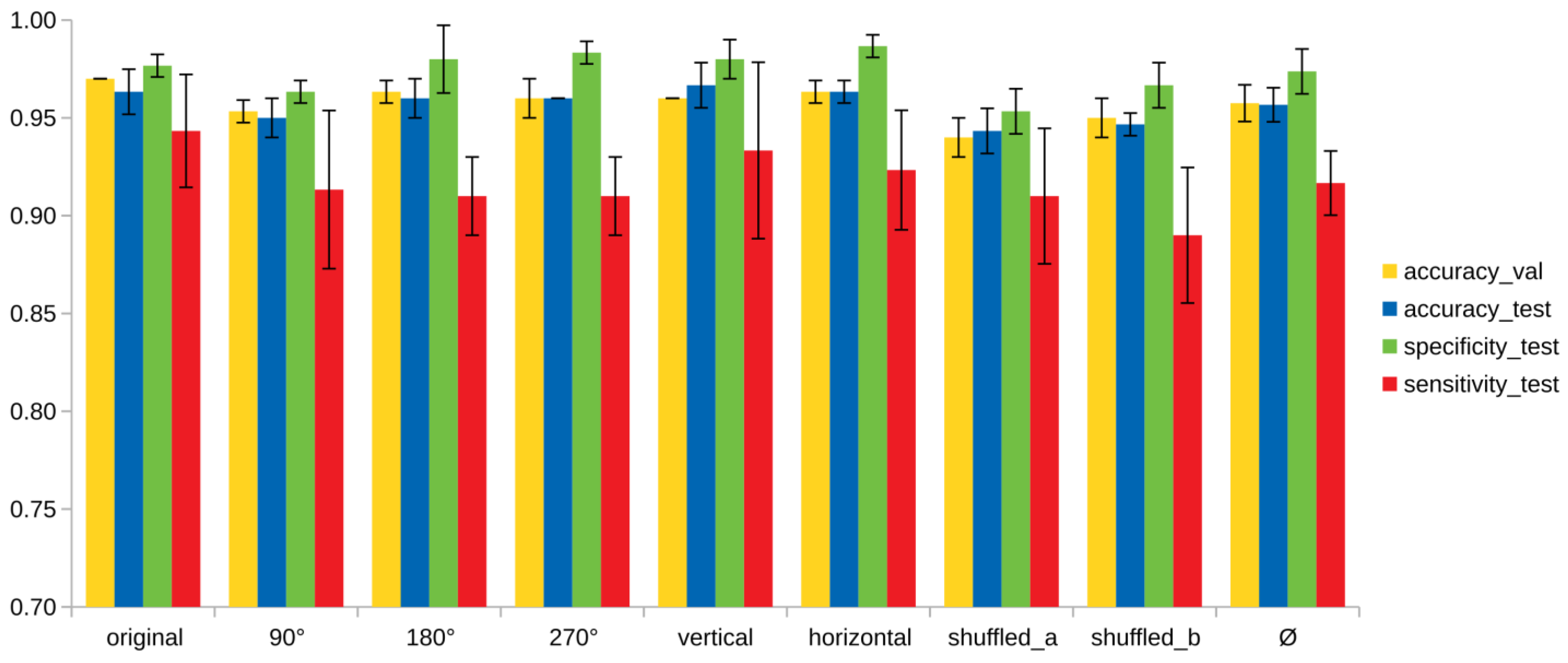
| Model | Validation Set | Test Set | Specificity | Sensitivity |
|---|---|---|---|---|
| original | 0.97 ± 0.00 | 0.96 ± 0.01 | 0.98 ± 0.01 | 0.94 ± 0.03 |
| 90° | 0.95 ± 0.01 | 0.95 ± 0.01 | 0.96 ± 0.01 | 0.91 ± 0.04 |
| 180° | 0.96 ± 0.01 | 0.96 ± 0.01 | 0.98 ± 0.02 | 0.91 ± 0.02 |
| 270° | 0.96 ± 0.01 | 0.96 ± 0.00 | 0.98 ± 0.01 | 0.91 ± 0.02 |
| vertical | 0.96 ± 0.00 | 0.97 ± 0.01 | 0.98 ± 0.01 | 0.93 ± 0.05 |
| horizontal | 0.96 ± 0.01 | 0.96 ± 0.01 | 0.99 ± 0.01 | 0.92 ± 0.03 |
| shuffled_a | 0.94 ± 0.01 | 0.94 ± 0.01 | 0.95 ± 0.02 | 0.91 ± 0.03 |
| shuffled_b | 0.95 ± 0.01 | 0.95 ± 0.01 | 0.97 ± 0.01 | 0.89 ± 0.03 |
| Ø | 0.96 ± 0.01 | 0.96 ± 0.01 | 0.97± 0.01 | 0.92 ± 0.02 |
Disclaimer/Publisher’s Note: The statements, opinions and data contained in all publications are solely those of the individual author(s) and contributor(s) and not of MDPI and/or the editor(s). MDPI and/or the editor(s) disclaim responsibility for any injury to people or property resulting from any ideas, methods, instructions or products referred to in the content. |
© 2023 by the authors. Licensee MDPI, Basel, Switzerland. This article is an open access article distributed under the terms and conditions of the Creative Commons Attribution (CC BY) license (https://creativecommons.org/licenses/by/4.0/).
Share and Cite
Pfeil, J.; Siptroth, J.; Pospisil, H.; Frohme, M.; Hufert, F.T.; Moskalenko, O.; Yateem, M.; Nechyporenko, A. Classification of Microbiome Data from Type 2 Diabetes Mellitus Individuals with Deep Learning Image Recognition. Big Data Cogn. Comput. 2023, 7, 51. https://doi.org/10.3390/bdcc7010051
Pfeil J, Siptroth J, Pospisil H, Frohme M, Hufert FT, Moskalenko O, Yateem M, Nechyporenko A. Classification of Microbiome Data from Type 2 Diabetes Mellitus Individuals with Deep Learning Image Recognition. Big Data and Cognitive Computing. 2023; 7(1):51. https://doi.org/10.3390/bdcc7010051
Chicago/Turabian StylePfeil, Juliane, Julienne Siptroth, Heike Pospisil, Marcus Frohme, Frank T. Hufert, Olga Moskalenko, Murad Yateem, and Alina Nechyporenko. 2023. "Classification of Microbiome Data from Type 2 Diabetes Mellitus Individuals with Deep Learning Image Recognition" Big Data and Cognitive Computing 7, no. 1: 51. https://doi.org/10.3390/bdcc7010051