An Obstacle-Finding Approach for Autonomous Mobile Robots Using 2D LiDAR Data

Abstract

Obstacle detection is crucial for the navigation of autonomous mobile robots: it is necessary to ensure their presence as accurately as possible and find their position relative to the robot. Autonomous mobile robots for indoor navigation purposes use several special sensors for various tasks. One such study is localizing the robot in space. In most cases, the LiDAR sensor is employed to solve this problem. In addition, the data from this sensor are critical, as the sensor is directly related to the distance of objects and obstacles surrounding the robot, so LiDAR data can be used for detection. This article is devoted to developing an obstacle detection algorithm based on 2D LiDAR sensor data. We propose a parallelization method to speed up this algorithm while processing big data. The result is an algorithm that finds obstacles and objects with high accuracy and speed: it receives a set of points from the sensor and data about the robot’s movements. It outputs a set of line segments, where each group of such line segments describes an object. The two proposed metrics assessed accuracy, and both averages are high: 86% and 91% for the first and second metrics, respectively. The proposed method is flexible enough to optimize it for a specific configuration of the LiDAR sensor. Four hyperparameters are experimentally found for a given sensor configuration to maximize the correspondence between real and found objects. The work of the proposed algorithm has been carefully tested on simulated and actual data. The authors also investigated the relationship between the selected hyperparameters’ values and the algorithm’s efficiency. Potential applications, limitations, and opportunities for future research are discussed.

1. Introduction

The development of autonomous mobile robots is increasingly attracting the attention of large groups of researchers. As is known [1,2,3,4,5], an autonomous mobile robot is an automatic device designed to perform industrial, transport, medical, military, space, and other operations, usually without human intervention. To complete the required tasks [6,7,8], this type of robot involves complex algorithms, such as algorithms for localization, navigation, control of the mechanical arm, the behaviour of combat robots, and service robotics. The input data are from sensors: cameras, humidity sensors, temperature sensors, GPS, and LiDAR. The algorithm developed and described in this paper uses information from the latest research (see Table 1).

LiDAR, which stands for Light Detection and Ranging, is a type of sensor that uses laser beams to measure distances and create precise maps of the environment. The basic principle of LiDAR is to emit laser beams and measure the time it takes for the light to reflect back to the sensor, allowing it to calculate the distance to objects. LiDAR sensors are typically composed of several components, including a laser source, a scanner, and a receiver. The laser emits a beam of light that is directed by the scanner towards the environment to be mapped. When the laser beam hits an object, some of the light is reflected back towards the sensor, where it is detected by the receiver. The time it takes for the light to return to the sensor is used to calculate the distance to the object. By repeating this process many times, a map of the environment can be created. LiDAR sensors are commonly used in a wide range of applications, including robotics, autonomous vehicles, surveying, and 3D mapping. They are especially useful in environments where other sensors, such as cameras or radar, may be less effective, such as in low-light conditions or when the environment is cluttered with obstacles.

LiDAR sensors are divided into two main types: 2D LiDAR and 3D LiDAR. The main difference between 2D and 3D LiDAR is the level of detail that can be captured and the types of information that can be extracted from the data.

Two-dimensional LiDAR, as the name suggests, captures data in two dimensions, typically creating a top-down view of the environment. The laser scanner rotates or oscillates to capture a 360-degree field of view, but the resulting data consist of a flat 2D map of the environment. Two-dimensional LiDAR is useful for obstacle detection, mapping, and navigation, but it cannot capture the full depth and shape of objects in the environment.

Three-dimensional LiDAR, on the other hand, captures data in three dimensions, creating a detailed map of the environment that includes depth information. This allows for more precise measurements of the distance between objects, as well as the shape and size of the objects themselves. Three-dimensional LiDAR is useful for a wider range of applications, including object recognition, tracking, and classification.

In addition to the difference in the level of detail captured, 2D and 3D LiDAR sensors also differ in their cost and complexity. Two-dimensional LiDAR sensors are generally simpler and less expensive than 3D LiDAR sensors, making them more suitable for some applications where high precision 3D data are not required. Overall, the choice between 2D and 3D LiDAR will depend on the specific application and the level of detail required. Two-dimensional LiDAR is often used in applications such as robotics and mapping, while 3D LiDAR is more commonly used in autonomous vehicles, industrial automation, and other applications that require highly detailed 3D data.

Many works have been written about finding obstacles using data from a 3D LiDAR sensor. Zermas et al. proposed a pipeline that aims to solve the problem of 3D point cloud segmentation for data received from LiDAR in a fast and low-complexity manner that targets real-world applications [9]. The two-step algorithm first extracts the ground surface in an iterative fashion using deterministically assigned seed points, and then clusters the remaining non-ground points taking advantage of the structure of the LiDAR point cloud. Himmelsbach et al. proposed a method for segmentation of 3D point clouds by labeling scanned points as either ground or non-ground [10]. The algorithm estimates the local ground plane by applying 2D line extraction algorithms to the domain of unorganized 3D points. This allows non-ground points to be separated from ground points, improving the accuracy of the segmentation process. Overall, the algorithm offers a promising approach to segmenting 3D point clouds, which has important applications in robotics, mapping, and other fields. Despite the advantages of 3D LiDAR in terms of its ability to capture detailed 3D information about the environment, there are also some limitations to its use. One of the main challenges with 3D LiDAR is that the data it captures are large and complex, which can result in longer processing times and higher computational requirements.

Two-dimensional LiDAR sensors are most often installed either horizontal-looking or downward-looking. The main difference between downward-looking 2D LiDAR and horizontal-looking 2D LiDAR is the direction in which they capture data. Downward-looking 2D LiDAR is mounted above the ground and captures data in a vertical direction, providing information about the height and profile of the ground surface, as well as any obstacles on it. In contrast, horizontal-looking 2D LiDAR is mounted on the side of a vehicle or robot and captures data in a horizontal direction, providing information about obstacles and features in the environment at the same level as the sensor.

Pang et al. proposed a method for downward-looking 2D LiDAR sensor [11]. The method begins by extracting line segments from the raw sensor data, and then estimates the height and the vector of the scanned road surface at each moment. Subsequently, the segments are divided into either road ground or obstacles based on the average height of each line segment and the deviation between the line segment and the road vector estimated from the previous measurements. Liu et al. [12] developed an algorithm for creating a local digital elevation map using downward-looking LiDAR sensors. The algorithm calculated the average height of points in voxels and extracted candidate road curbs based on the height variance and slope of adjacent voxels. While the algorithm demonstrated good experimental results, it was found to be less effective in dealing with complex curved slopes and changing road conditions, such as sloping roads with sharp turns.

The algorithm described in this work was developed for use by an autonomous mobile robot of a small size that operates indoors. A horizontal-looking 2D LiDAR sensor is best suited for such a setup. For example, Baek et al. use similar maintenance for robotic vacuum cleaners [13], which are very popular today. The advantages of a horizontal-looking 2D LiDAR sensor compared to a downward-looking 2D LiDAR sensor include:

• Coverage: Horizontal-looking 2D LiDAR sensors provide a 360-degree field of view, which makes them better suited for applications where a full view of the environment is required. Downward-looking 2D LiDAR sensors, on the other hand, have a more limited view and can miss obstacles outside of their field of view.
• Obstacle detection: Horizontal-looking 2D LiDAR sensors are better suited for detecting obstacles on the ground or at low heights, such as curbs, speed bumps, or potholes. Downward-looking 2D LiDAR sensors are better suited for detecting objects directly below the sensor, such as the ground or a floor.

An instance of how a 2D LiDAR sensor can be used is an algorithm designed to determine the sensor’s current position [14] accurately. The algorithm uses OpenMP parallel computing technology to increase its processing speed and achieve real-time results.

Objective research proposed by Leigh et al. [15] promotes the development of robust, repeatable, and transferable software for robots that can automatically detect, track, and follow people in their environment. They propose a new algorithm for robust detection, tracking, and following from 2D LiDAR data. We show that the approach is effective in various environments, both indoor and outdoor, and on different robot platforms (the intelligent power wheelchair and a Clearpath Husky). The method has been implemented in the Robot Operating System (ROS) framework and will be publicly released as a ROS package. The autonomous person detection is achieved using clustering. The autonomous tracking is achieved using a combination of Kalman filter and a GNN method.

Catapang et al. developed a low-cost 2D LiDAR system for detecting obstacles in autonomous vehicles. The system is designed to acquire data in a single plane, resulting in fast computational processing. The LiDAR system provides a wide field of view of up to 360 degrees. The acquired data were pre-processed by merging and segmenting data points and then median-filtered. Obstacle detection was performed using clustering algorithms. The results demonstrated that the developed LiDAR system can detect obstacles with a width of 1 m at a distance of 10 m. Chung et al. proposed an algorithm for detecting human legs and tracking them with a single laser range finder. The human legs were detected by the application of a support vector data description scheme, and it tracked the leg positions according to an analysis of human walking motion [16].

Table 1. An overview of related works.

Reference	Sensor	Method	Advantages	Disadvantages
Zermas et al. [9]	3D LiDAR	Iterative fashion using deterministically assigned seed points	Lots of useful information about the environment	Expansive and height processing time
Himmelsbach et al. [10]	3D LiDAR	Labeling scanned points as either ground or non-ground
Pang et al. [11]	Downward-looking 2D LiDAR	Divide into either road ground or obstacles based on the average height of each line segment	A method to effectively deal with obstacles of different heights on city roads	Some limitations in distinguishing dynamic obstacles such as pedestrians
Liu et al. [12]	Downward-looking 2D LiDAR	Quantized digital elevation map and grayscale reconstruction	Data processing by using existing image processing techniques	Not discuss the conversion between different scenes
Leigh et al. [15]	Horizontal-looking 2D LiDAR	Clustering to detect object and combination of Kalman filter and a GNN to track object	Implementation of the algorithm for ROS	Designed only for detection of a certain type of obstacles
Catapang et al. [17]	Horizontal-looking 2D LiDAR	Median filter for pre-processing and clustering for obstacles detecting	The algorithm works well on objects that are far from the sensor	It is not enough visualization of the result of the algorithm on data from real sensor
Chung et al. [16]	Horizontal-looking 2D LiDAR	Support vector data description	No geometric assumption and the robust tracking of dynamic object	Designed only for detection of a certain type of obstacles

Table 1. An overview of related works.

Reference	Sensor	Method	Advantages	Disadvantages
Zermas et al. [9]	3D LiDAR	Iterative fashion using deterministically assigned seed points	Lots of useful information about the environment	Expansive and height processing time
Himmelsbach et al. [10]	3D LiDAR	Labeling scanned points as either ground or non-ground
Pang et al. [11]	Downward-looking 2D LiDAR	Divide into either road ground or obstacles based on the average height of each line segment	A method to effectively deal with obstacles of different heights on city roads	Some limitations in distinguishing dynamic obstacles such as pedestrians
Liu et al. [12]	Downward-looking 2D LiDAR	Quantized digital elevation map and grayscale reconstruction	Data processing by using existing image processing techniques	Not discuss the conversion between different scenes
Leigh et al. [15]	Horizontal-looking 2D LiDAR	Clustering to detect object and combination of Kalman filter and a GNN to track object	Implementation of the algorithm for ROS	Designed only for detection of a certain type of obstacles
Catapang et al. [17]	Horizontal-looking 2D LiDAR	Median filter for pre-processing and clustering for obstacles detecting	The algorithm works well on objects that are far from the sensor	It is not enough visualization of the result of the algorithm on data from real sensor
Chung et al. [16]	Horizontal-looking 2D LiDAR	Support vector data description	No geometric assumption and the robust tracking of dynamic object	Designed only for detection of a certain type of obstacles

This study aims to develop a precise obstacle detection algorithm utilizing data from a horizontal-looking 2D LiDAR sensor. The algorithm is designed to run on low-powered computers and is specifically tailored for use in an indoor setting, such as an autonomous mobile robot.

Two primary metrics will be used to assess accuracy. The first metric is Cluster Homogeneity [18]. The second metric is Cluster Completeness [19].

Cluster Homogeneity and Cluster Completeness are two metrics used to evaluate the quality of a clustering algorithm’s performance.

Cluster Homogeneity measures the extent to which all data points within a cluster belong to the same class or category. If all points in a cluster belong to the same class, then the cluster is said to be homogeneous. A score of 1.0 indicates perfect homogeneity, while a score closer to 0.0 indicates lower homogeneity.

Cluster Completeness, on the other hand, measures the extent to which all data points belonging to the same class are assigned to the same cluster. If all data points belonging to a given class are assigned to the same cluster, then the clustering is said to be complete. A score of 1.0 indicates perfect completeness, while a score closer to 0.0 indicates lower completeness.

Both Cluster Homogeneity and Cluster Completeness are evaluated on a scale from 0.0 to 1.0, with higher scores indicating better performance. These metrics are commonly used in unsupervised machine learning tasks, such as clustering and topic modeling, to evaluate the accuracy of the algorithm’s predictions.

Although the Cluster Homogeneity and Cluster Completeness metrics are useful for evaluating the accuracy of the algorithm’s output compared to the real environment, they should not be the only consideration when using the algorithm in production. Instead, the visualization of the algorithm’s output and the specific requirements of the task should guide the selection of hyperparameters. For instance, certain hyperparameter configurations may be more appropriate for real-time navigation while others may be better suited for calculating the robot’s movement vector during the LiDAR sensor’s scanning period.

The main contributions of this article can be summarized as follows:

• A linear-complexity algorithm for obstacle detection was developed using data from a 2D LiDAR sensor, which is capable of working with high-frequency sensors;
• A parallelization method is proposed for the developed algorithm, which makes it possible to reduce the time of operation of one iteration of the algorithm in proportion to the number of cores used;
• A simulator was developed for testing the algorithm, which helps to test hypotheses and quickly select hyperparameters for the given task;
• Clustering quality metrics were used to assess the accuracy of the result of solving obstacles in the task search.

The rest of this article is organized as follows: Section 2 presents the proposed algorithm. Section 3 describes the test data. Section 4 describes the results in detail. Conclusions and prospects for further research are shown in the last section.

2. Materials and Methods

2.1. Statement of the Research

As mentioned above, LiDAR is a technology for obtaining and processing information about remote objects. Data from the LiDAR sensor are usually represented as a vector of angles and a vector of distance at the appropriate angle, that is, in the polar coordinate system:

$$\begin{array}{c}\theta =\left({\theta }_1,{\theta }_2,\dots ,{\theta }_n\right),\\ d=\left(d_1,d_2,\dots ,d_n\right).\end{array}$$

where $n$—is the number of measured distances when scanning the room, $\theta$—is the vector of angles, and $d$—is the vector of distances. This data can be converted into points $(x_i, y_i)$ in the Cartesian coordinate system, where

$$\left.\begin{array}{c}{x}_i=d_i\cos {\theta }_i \\ y_i=d_i\sin {\theta }_i \end{array}\right\} i\in \left[1,n\right]$$

(1)

Thus, the points $\left(x_i, y_i\right)$ at the end of the beams relative to the position of the robot during scanning are obtained. Also, the necessary data for the developed algorithm are the robot displacement vector $S=(S_x, S_y, S_{\phi })$ from the previous scan by the LiDAR sensor to the current one. The value of this displacement vector may have an error [20] (as a rule, it is impossible to calculate the distance travelled by the robot accurately).

We will call the history at the time of the current scan at number $m$ the present, and all previous scans and moves:

$$H_m=〈{\theta }^{(1)}, d^{(1)}, \dots , S^{(m)}, {\theta }^{(m)}, d^{(m)}〉.$$

(2)

The superscript will specify the scan number in parentheses.

Based on the previous definitions, the purpose of this work can be formulated: using the history of all robot movements and data from the LiDAR sensor, find the set $O$, where each element of the group is a set of segments that corresponds to the obstacle description. Obstacles found by the algorithm should be as accurate as possible.

Solving this problem consists of three main steps:

• Elimination of obsolete points from the LiDAR sensor;
• Clustering of sifted points;
• Finding the contours of each cluster.

2.2. Elimination of Obsolete Points from the LIDAR Sensor

First of all, it is necessary to find the positions of the issues from the previous scans relative to the work at the moment of the scanning $m$. To do this does not to take into account all movements between the previous $\left(x_i^{(j)}, y_i^{(j)} \right)$ and the last $\left({\widehat{x}}_i^{\left(j\right)}, {\widehat{y}}_i^{\left(j\right)} \right)$ scan, where

$$\left.\begin{array}{c}{\widehat{x}}_i^{\left(j\right)}=x_i^{\left(j\right)}+{\displaystyle \sum }_{k=j+1}^m{S}_x^{\left(k\right)} \\ {\widehat{y}}_i^{\left(j\right)}=y_i^{\left(j\right)}+{\displaystyle \sum }_{k=j+1}^m{S}_y^{\left(k\right)}\end{array}\right\}i\in \left[1,n^{\left(j\right)}\right].$$

(3)

Since the next part of the algorithm requires points in the polar coordinate system, the result Equation (3) must be transformed into it:

$$\left.\begin{array}{c}{\widehat{\theta }}_i^{\left(j\right)}={\tan }^{-1}\frac{{\widehat{y}}_i^{\left(j\right)}}{{\widehat{x}}_i^{\left(j\right)}} \\ {\widehat{d}}_i^{\left(j\right)}=\sqrt{{\left({\widehat{x}}_i^{\left(j\right)}\right)}^2+{\left({\widehat{y}}_i^{\left(j\right)}\right)}^2}\end{array}\right\} i\in \left[1,n^{\left(j\right)}\right].$$

(4)

As mentioned earlier, the displacement vector has a measurement error, which is the reason for the elimination of points. Those points scanned earlier should be less likely to get to the next stage of the algorithm. This can be realized by defining a hyperparameter $\gamma \in \left[0, 1\right]$. Then, the probability of the $i$-th point from the j-th getting into the set $A$ can be determined as follows:

$$p_i^{(j)}={\gamma }^{m-j}.$$

Consequently, the set $A$ is less likely to contain points that were scanned earlier.

2.3. Clustering of Sifted Points

In the obstacle detection algorithm, clustering is a crucial step that determines which points belong to an obstacle. This process must be efficient enough to be executed between LiDAR sensor scans, and it should also have adjustable hyperparameters that can be modified according to the sensor configuration. In this section, a clustering algorithm based on the components of the connectivity search method is proposed. The following section will compare this approach to other clustering methods such as DBSCAN [21] and K-Means [22], which can also be utilized in the final algorithm.

First, the clustering algorithm requires normalized data since the elements of the set $A$ are vectors in the polar coordinate system. The components of such a vector have different units (radians and units of distance). Therefore, a group with normalized vectors is defined as follows:

$$\tilde{A}=\left\{\left(\theta , d\right)\in A\left|\left(\theta ,\frac{d-\overline{d}}{{\sigma }_d}\right)\right.\right\},$$

where $\overline{d}$, ${\sigma }_d$—the average distance and the variance of the length overall vectors of the set $A$. Also, to perform clustering, you need to set the distance function between two vectors of the group $\tilde{A}$. The following distance function was proposed:

$$f\left(\left({\theta }_1,d_1\right), \left({\theta }_2, d_2\right)\right)=\sqrt{\rho {({\cos }^{-1}\left(\cos \left({\theta }_1-{\theta }_2\right)\right))}^2+\left(1-\rho \right){\left(d_1-d_2\right)}^2},$$

(5)

where $\rho \in \left[0, 1\right]$—hyperparameter that determines the balance between two quantities. Now, the graph $G=\left(\tilde{A},E\right)$ can be evaluated, where $\tilde{A}$ is a set of vertices (vertices will be considered points in the polar coordinate system), and $E$ is a set of edges. Between two vertices $a_1,a_2$ there is an edge if and only if the distance Equation (5) between them is less than $\xi$:

$$E=\left\{\left.\left(a_1, a_2\right)\right|a_1\in \tilde{A} \mathrm{and} a_2\in \tilde{A} \mathrm{and} f \left(a_1, a_2\right)<\xi \right\} .$$

In the final part of this stage, the basic algorithm on the graphs that finds the components of connectivity—DFS [23] needs to be used. The algorithm used in this implementation was chosen based on the task’s requirements and the characteristics of the LiDAR sensor. The DFS-based connectivity component search algorithm was found to be the most suitable due to the low error of the LiDAR sensor, as points belonging to one object generally fall into one cluster. However, if the distance error of the LiDAR sensor is large, DBSCAN may be more optimal. It can also identify some points as outliers.

The output of the algorithm is a set of clusters. Each cluster is a set of points that are part of it:

$$B=\left\{B_1, B_2, \dots , B_c\right\}$$

where c—the number of clusters that the algorithm will find.

2.4. Finding the Contours of Each Cluster

The result of the previous stage of the algorithm is a set of clusters $B$. The next and final step of the proposed algorithm is to obtain a set of line segments, where each group is responsible for describing the obstacle.

Consider a cluster $B_i$. The vectors are sorted by increasing angle: ${\theta }_1\le {\theta }_2\le \dots \le {\theta }_l, l=\left|B_i\right|.$ The kernel of length $\alpha \in N$ by the number $k$ is the set $B_{{}_i}^{\left(k\right)}=\left\{\left({\theta }_k, d_k\right), \dots , \left({\theta }_{k+\alpha -1}, d_{k+\alpha -1}\right)\right\}.$ Denote the mean angle of the kernel ${\overline{\theta }}^{(k)}:=\frac{1}{\alpha }{\displaystyle \sum _{j=k}^{k+\alpha -1}{\theta }_j}$. Denote by the maximum and minimum distance of the kernel $d_{\max }^{\left(k\right)}:=\max \left(d_k, \dots , d_{k+\alpha -1}\right),$ $d_{\min }^{\left(k\right)}:=\min \left(d_k, \dots , d_{k+\alpha -1}\right),$ respectively. The final location $O_i$ of the segments responsible for the expected obstacle can be specified as a union of three sets:

$$\begin{gathered} O_i=O_i^{(\min )}\cup O_i^{(\max )}\cup O_i^{(\mathrm{merge})}; O_i^{(\min )}= \\ \left\{\left[\left({\overline{\theta }}^{(1)}, d_{\min }^{(1)}\right), \left({\overline{\theta }}^{(2)}, d_{\min }^{(2)}\right)\right], \right.\left[\left({\overline{\theta }}^{(2)}, d_{\min }^{(2)}\right), \left({\overline{\theta }}^{(3)}, d_{\min }^{(3)}\right)\right], \\ \left.\dots , \left[\left({\overline{\theta }}^{(c-\alpha -1)}, d_{\min }^{(c-\alpha -1)}\right), \left({\overline{\theta }}^{(c-\alpha )}, d_{\min }^{(c-\alpha )}\right) \right]\right\};O_i^{(\max )}= \\ \left\{\left[\left({\overline{\theta }}^{(1)}, d_{\max }^{(1)}\right), \left({\overline{\theta }}^{(2)}, d_{\max }^{(2)}\right)\right], \right.\left[\left({\overline{\theta }}^{(2)}, d_{\max }^{(2)}\right), \left({\overline{\theta }}^{(3)}, d_{\max }^{(3)}\right)\right], \\ \left.\dots , \left[\left({\overline{\theta }}^{(c-\alpha -1)}, d_{\max }^{(c-\alpha -1)}\right), \left({\overline{\theta }}^{(c-\alpha )}, d_{\max }^{(c-\alpha )}\right) \right]\right\};O_i^{(\mathrm{merge})}= \\ \left\{\left[\left({\overline{\theta }}^{(1)}, d_{\min }^{(1)}\right), \left({\overline{\theta }}^{(1)}, d_{\max }^{(1)}\right)\right], \left[\left({\overline{\theta }}^{(c-\alpha )}, d_{\min }^{(c-\alpha )}\right), \left({\overline{\theta }}^{(c-\alpha )}, d_{\max }^{\left(c-\alpha \right)}\right)\right]\right\}. \end{gathered}$$

The set $O_i^{(\min )}$ is responsible for the part of the obstacle that is closer to the LiDAR sensor. “Closer” means that a line segment can be drawn between the position of the sensor and any point belonging to any element $O_i^{}$ that will not intersect with any other object $O_i^{}$. The set $O_i^{(\max )}$ is responsible for the interference part that is farther from the LiDAR sensor. “Farther” means that there are an infinite number of points belonging to the polynomials $O_i^{(\max )}$ and the segment between any of them, and the position of the leader intersects with one object from $O_i^{(\min )}$ The set $O_i^{(\mathrm{merge})}$ is responsible for merging the two previous sets to obtain a polygon in the union. It is useful to obtain a polygon in order to estimate the discrete obstacle probability distribution function then. For example, all points that are in this polygon will have a high probability of obstacles (see Algorithm 1).

Algorithm 1: Cluster Contouring

2.5. Estimation of Algorithm Complexity

Assessing the complexity does not consider the first stage of the algorithm (the elimination of obsolete points). Without loss of generality, it is assumed that now is the $j$-th step, and an infinite number of measures have been performed before that. Suppose $n$ new points are obtained at each iteration. Then, the mathematical expectation of the power of the set $A$ will be calculated as follows:

$$E\left[\left|A\right|\right]={\displaystyle \sum _{k=0}^{\infty }{\gamma }^{k}n=\frac{n}{1-\gamma }}$$

The next stage of the algorithm will work with $E\left[\left|A\right|\right]$ number of points. The paper describes the algorithm for searching for connectivity components based on the depth-first search algorithm. The complexity of this algorithm is $O\left(\left|\tilde{A}\right|+\left|E\right|\right)$, where $\tilde{A}$ is the set of vertices, and $E$ is the set of edges. Since only adjacent vertices will be connected, then $\left|E\right|\le \left|\tilde{A}\right|$. Then, the complexity at this stage $O\left(\left|\tilde{A}\right|+\left|E\right|\right)=O\left(\left|\tilde{A}\right|\right)=O\left(\frac{n}{1-\gamma }\right)$. The last step of the algorithm will occur in each cluster $\alpha$ times, and therefore the final complexity of the algorithm will be $O\left(\frac{n}{1-\gamma }+\alpha \frac{n}{1-\gamma }\right)=O\left(\frac{1+\alpha }{1-\gamma }n\right)$.

Therefore, the complexity of the algorithm is linear concerning $n$. At the same time, it should be noted that no field discretization will be performed, which was completed in the works above, which is the reason for the prolonged execution of the algorithm. In the described method, all actions are performed on the initial data, which indicates high efficiency. In other words, to increase accuracy, the considered works sacrifice a lot of speed and memory because they need to iterate over the tabulated space, which the proposed algorithm does not do. Also, all these steps can be easily parallelized relative to the number of points, further increasing the iteration speed.

Therefore, a method of finding obstacles was proposed in this section. It is very flexible as it has enough hyperparameters to optimize it for the specific configuration of the LiDAR sensor. Namely, the algorithm has the following hyperparameters: γ—to set the degree of elimination of obsolete points, $\rho$—to set the balance between angle and distance for correct clustering, $\xi$—to set the threshold for creating an edge in the graph for the algorithm for finding connectivity components, α—to set the length of the kernel to determine the segments responsible for the obstacle.

2.6. Parallelization

It should be noted that each of the stages of the algorithm is very easy to divide into CPU cores and, at the same time, obtain extra acceleration. The first step is to search all list elements and delete them, provided that the Bernoulli experiment at a given probability will give 1. It is easy to parallelize using thread-safe collections (in this case, a double-linked list) [24].

To parallelize the second stage, an efficient multi-threaded DBSCAN algorithm [25] will be used. The idea is to divide the two-dimensional space into sectors, process each of the sectors in a separate thread, and finally use an algorithm for merging all sectors, which works for a time proportional to the number of sectors. Since the number of sectors is usually not large (equal to the number of cores), the merging time can sometimes be neglected.

The third stage is relatively easy to divide into cores if they are less than the number of clusters. For example, the first thread for the $i$-th cluster will handle the set $O_i^{(\min )}$, the second thread will take the $O_i^{(\max )}$, and the third and fourth will already work with the $i+1$ cluster. In this way, the process is evenly distributed between the cores. If you store sets in a double-linked list, you can then combine them in a constant time. Also, pay attention to the group $O_i^{(\mathrm{merge})}$. It always contains two elements, so the processing time can be considered consistent. Thus, the final complexity is $O\left(\frac{1+\alpha }{T(1-\gamma )}n\right)$. In the denominator, $T$—threads number appears.

2.7. Accuracy Metrics

Two primary metrics will be used to assess accuracy. The first metric is Cluster Homogeneity [18]. The second metric is Cluster Completeness [19]. Both metrics will give the ability to numerically see how many obstacles found by the algorithm are actual.

3. Data for Testing

This section describes data for testing. Two types of data were used: simulated and actual. Simulations were used to quickly verify the algorithm’s accuracy and empirical assessment of complexity and precision for quality estimation. Consider both types of data.

3.1. LIDAR Sensor Simulation for Testing

To simulate the LiDAR sensor, a set of segments was used to represent obstacles. The simulation algorithm is straightforward and does not require much computational power. It takes as input a set of obstacle segments, the robot’s position, and the number of LiDAR sensor rays. The output is a set of points that simulate the sensor, with their position matching the robot’s position.

3.2. Physical LIDAR Sensor for Testing

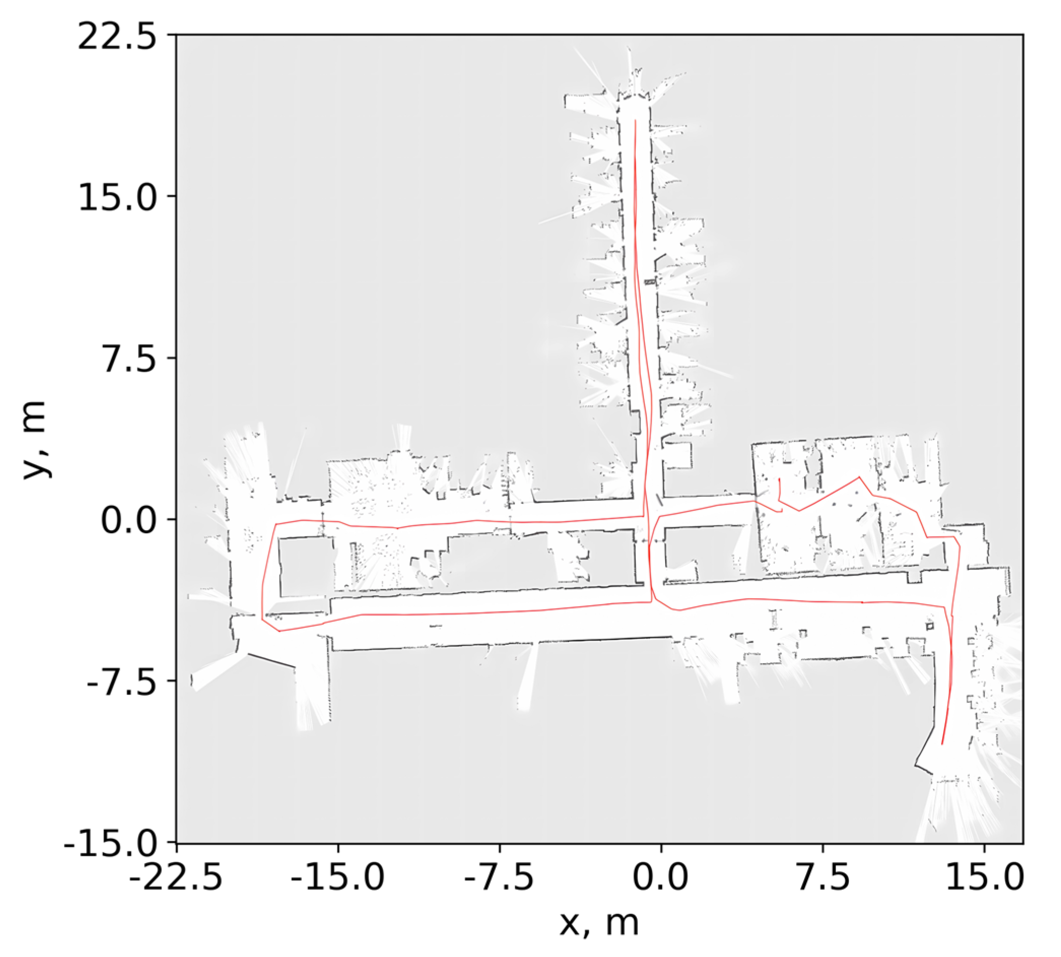
In this study, data were collected using a physical LiDAR sensor, specifically the SLAMTEC RPLIDAR A2, which had an operating frequency of 10 Hz. Typically, the device generated an output of approximately 300 points. The simulation was designed to mimic this behaviour and generated a similar number of points.

Red indicates the robot’s trajectory, and black shows the data from the leader (see Figure 1).

4. Results

This section is devoted to the results of testing the algorithm. It consists of two sections. The first section describes the results of testing on simulated data with visual visualization of the influence of the number of points from the LiDAR sensor on the algorithm’s complexity and visualization of specific cases without reducing the generality. The second section shows how the algorithm handles actual data.

4.1. Results on the Simulated Data

The first comparison was based on the following criterion: the result of the algorithm depends on the position of the LiDAR sensor relative to the obstacle. Input data were distances in centimetres and angles in radians. The following algorithm configuration was used: $\gamma =0.5$, $\rho =0.64$, ξ = 0.28, $\alpha =10$.

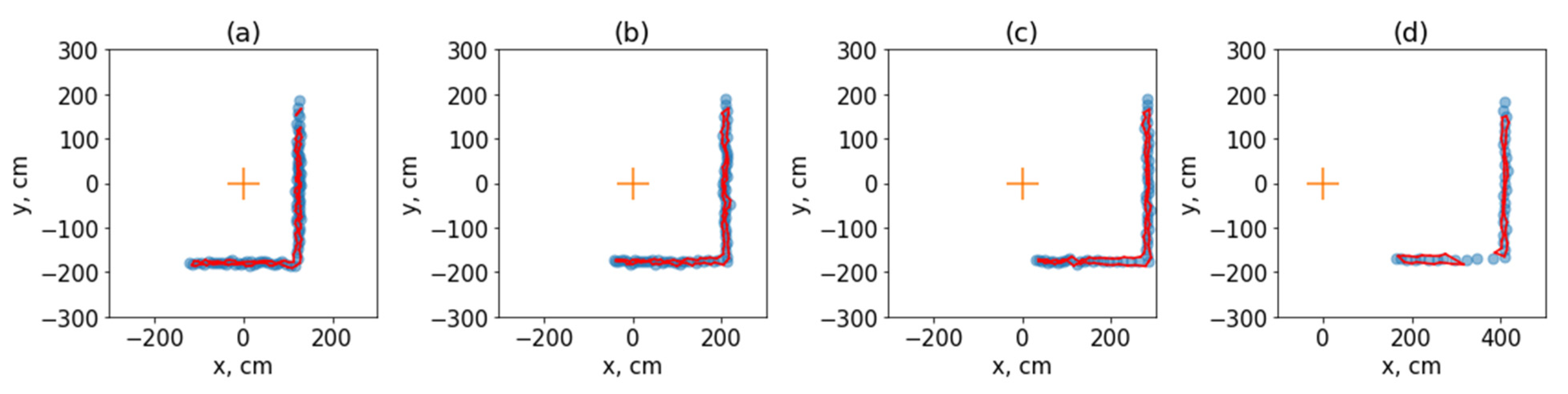
Figure 2 shows how the sensor’s position affects the algorithm’s result. The closer the sensor is to the obstacle, the better the polygon describes it. This is done to ensure that the sensors have a significant distance error [26,27,28]. If the sensor is placed as close as possible to the obstacle, the effect of angular error and distance error will be reduced, which gives the ability to determine the obstacle more accurately, as in case (a), where the resulting set of segments perfectly describes the points of the sensor. In case (d), where the obstacle is at a distance of 400 centimetres from the sensor, regarding the area of the two polygons, the algorithm considers the obstacles to be greater than in the previous cases. This means that the variance of the distance of the sensor, in this case, is quite large, and it is more advantageous to assume that the obstacle is more significant than it is. This will help the navigation algorithm to make plans that may not be rebuilt in the future [29].

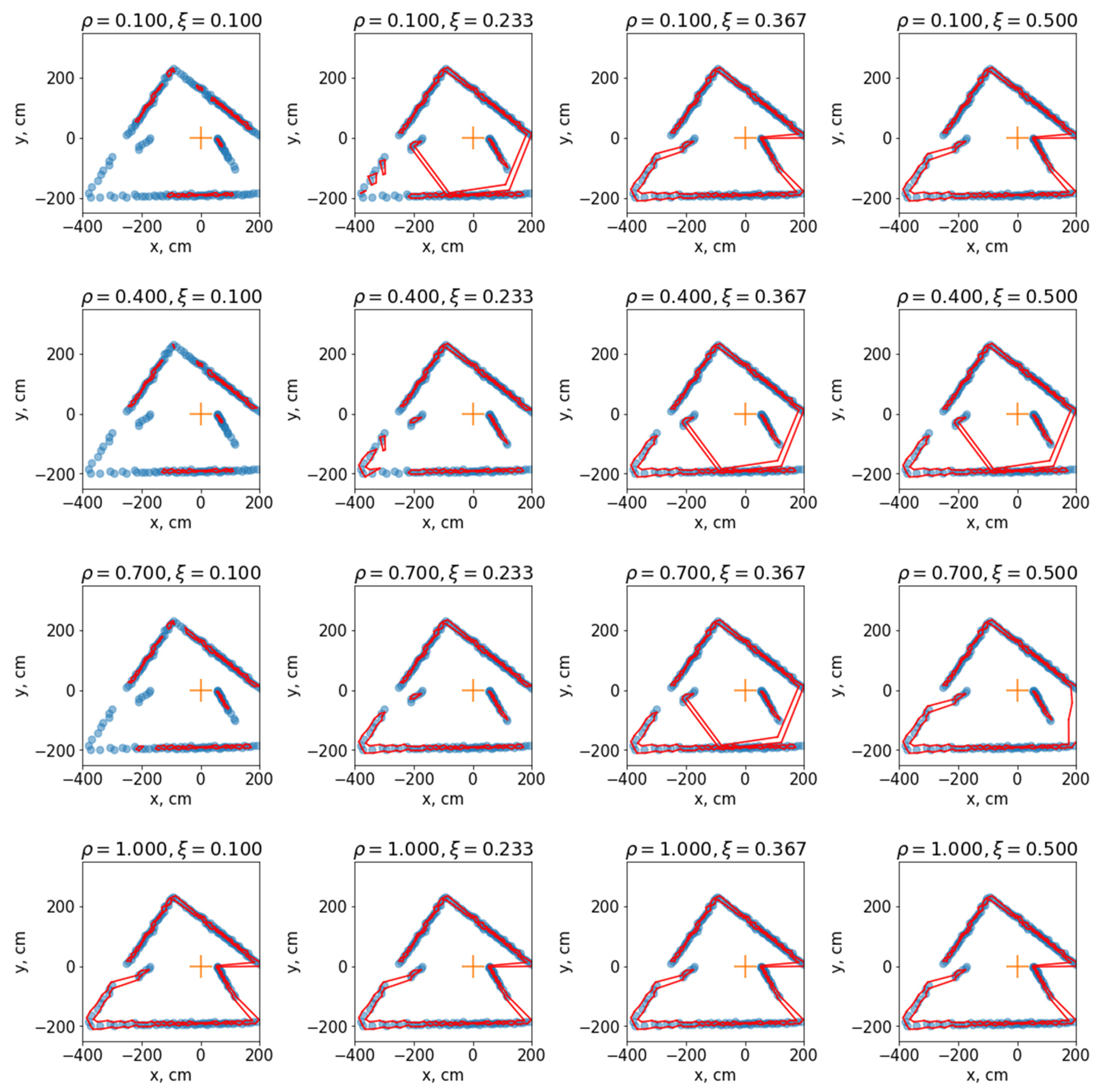
One of the essential steps to starting to use this method is the selection of hyperparameters. Next, how different combinations of hyperparameters affect the result of the algorithm will be shown. First, set $\gamma =0.5$ and α = 10. Let us take over all pairs $\rho \in \left\{0.1, 0.325, \dots , 1.0\right\},$ $\xi \in \left\{0.1, 0.2, \dots , 0.5\right\}$. For each pair, predictions on specific data from the sensor will be found.

Figure 3 shows the result of the algorithm with a specific configuration ρ and ξ. One of the best results was given by a set of hyperparameters of the algorithm γ = 0.5, α = 10, $\rho =0.775$, ξ = 0.2. As mentioned above, ρ sets the balance between angle and distance when clustering. When $\rho =1$, only the angles will be taken into account, so if the sensor is correct and the angular distances between adjacent points are equal to and less than a given threshold, the algorithm will return a single set of segments that describes the data from the sensor. This can be seen in the last five pictures. The ξ parameter specifies the edge creation threshold in the graph for the connectivity component search algorithm. If it is too small, only very clustered groups of points will be considered as clusters. Some individual points may be regarded as separate clusters. Due to the further specificity of the algorithm related to the search for contours, they will not be defined as obstacles at all. In the figure, this can be seen in the first column. The first four configurations do not consider some points. This may be necessary when there is a need to identify an obstacle that is close to the sensor.

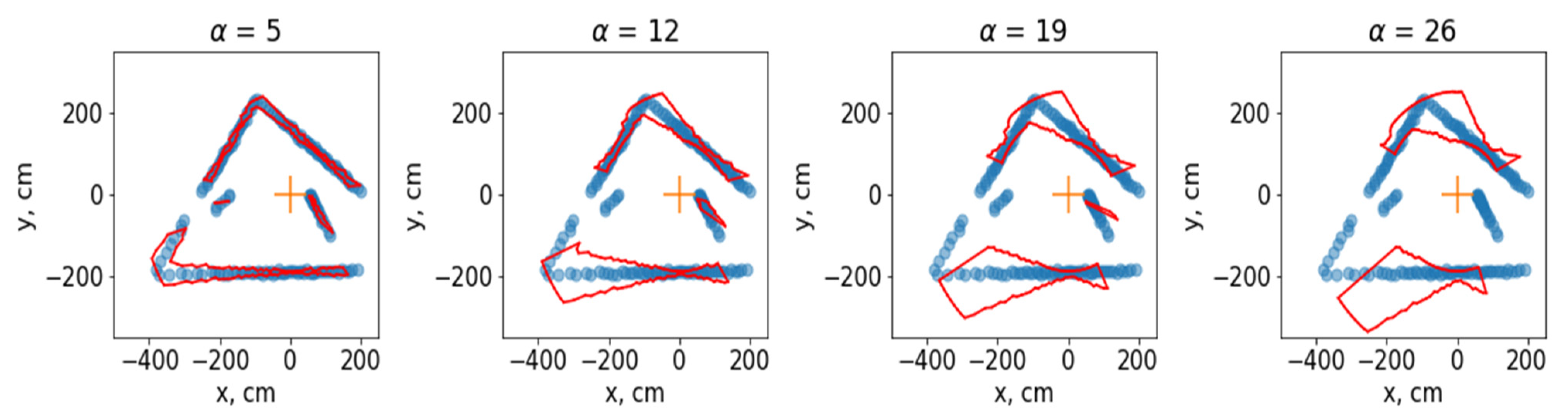
If hyperparameters are set γ = 0.5, ρ = 0.775, ξ = 0.2, visualization of the dependence between the result and the $\alpha$ hyperparameter will look like Figure 4.

Figure 4 clearly shows how the hyperparameter $\alpha$ affects the result of the work. Increasing it will favour large clusters. Also, with its significant increase, the area of the polygon increases significantly, which indicates the uncertainty of the position of the obstacle. It is also important to note that the length of the kernel should be set relative to the number of points returned by the LiDAR sensor. The greater the number of points, the greater the size of the cores must be set. Figure 4 shows 180 points from the LiDARs. For such a value, it is optimal to set $\alpha =5$. If the frequency of the sensor decreases, which will cause the number of points to increase, then $\alpha =12$ will be more optimal. Of course, it is better to select these values separately for each task.

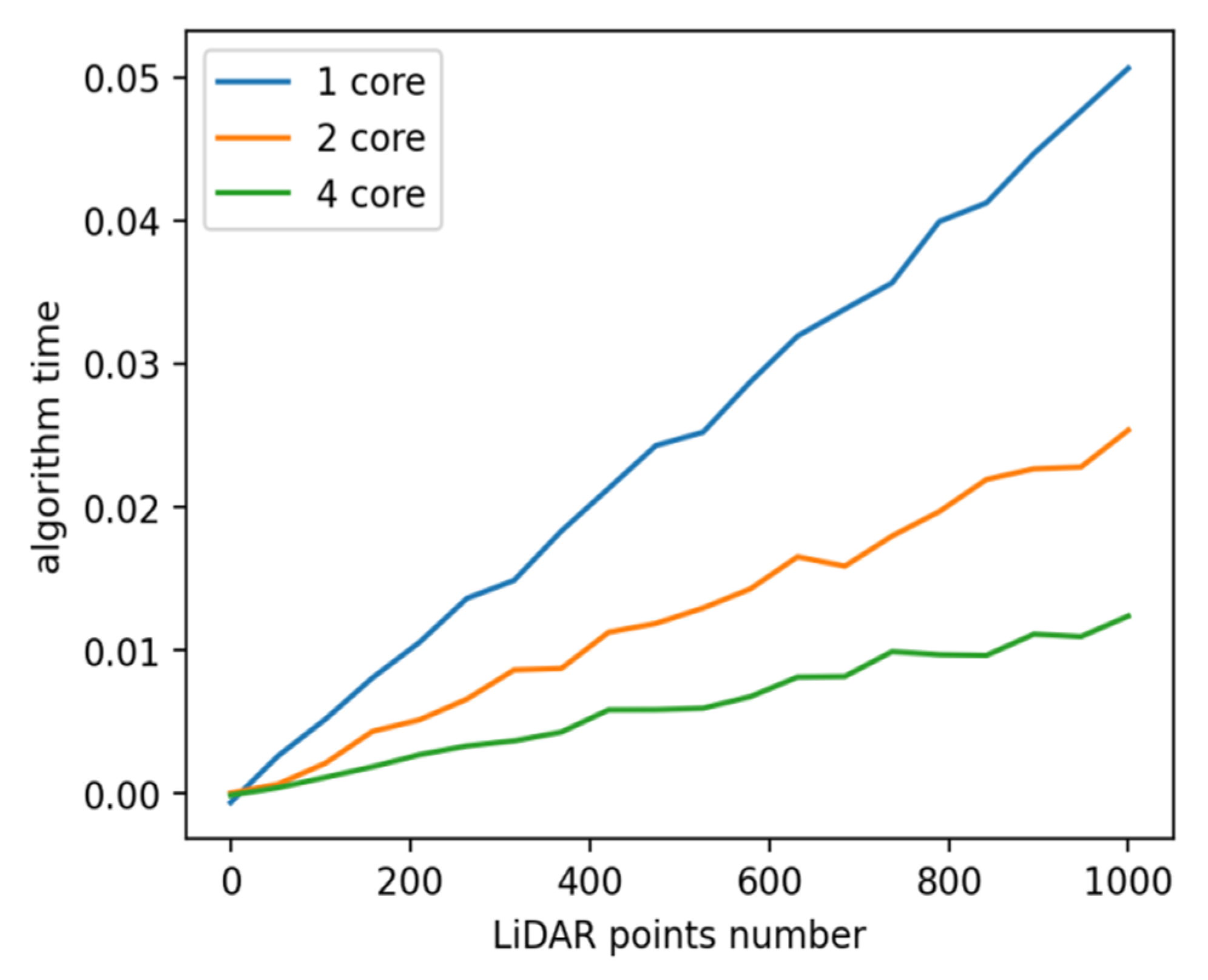
Figure 5 shows that the dependence is linear concerning the number of points, which confirms the proof in Section 2.5. During the complexity assessment, the hyperparameters were recorded and set γ = 0.5, $\alpha =10$, $\rho =0.775$, ξ = 0.2. It is also clear that parallelization reduces the running time of the algorithm, and the more cores, the less time.

4.2. Results on Actual Data

The results on actual data are pretty similar to the results of the simulation. This is primarily because a device such as a LiDAR sensor has a simple principle of operation that allows a quality simulation to be made [30].

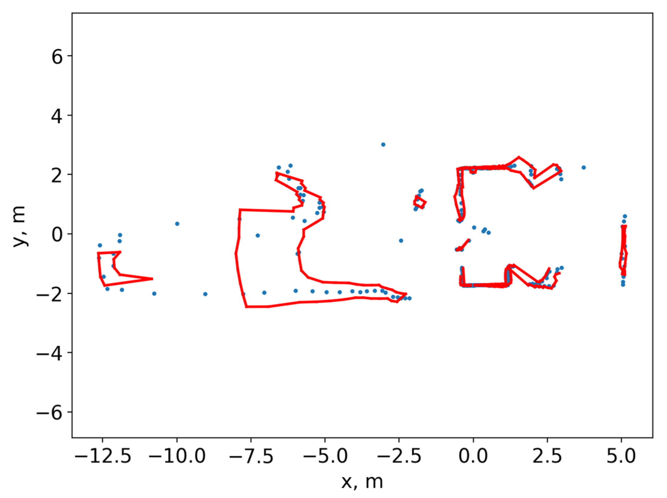
Figure 6 shows the result of the algorithm with hyperparameters γ = 0.5, $\alpha =5$, $\rho =0.640$, and $\xi =0.280$. Obviously, an algorithm with this configuration does not cope well with points far from the sensor. It is generally due to the sensor’s accuracy, as it drops sharply at a distance of more than nine metres. It would be appropriate to look at the dependence of the complexity of the algorithm on time. Section 2.5 mentions that the complexity depends on the parameter γ. The difficulty should increase gradually as some of the points from previous iterations are retained.

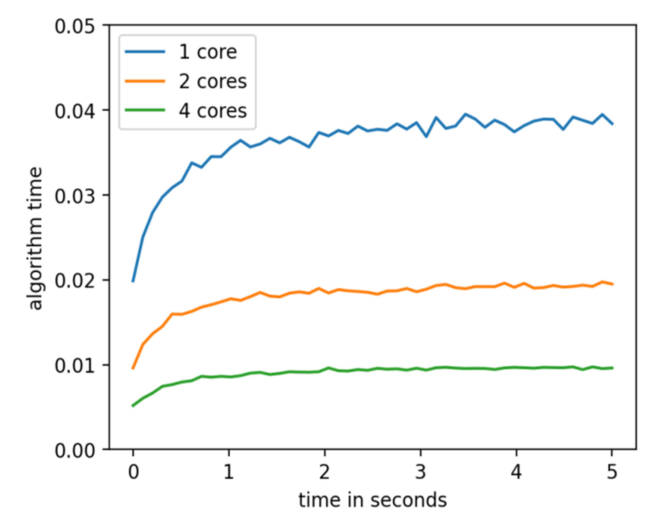
Figure 7 shows that the algorithm does its job longer but with a certain asymptote over time. After the second, the complexity stopped growing and was about 0.04 s for a single-core processor. The graphs also show that the number of cores directly affects the speed.

5. Conclusions

The article introduces an algorithm for object and obstacle detection using 2D LiDAR sensor data. The algorithm has a relatively low computational complexity, making it suitable for use in projects where autonomous mobile robots have limited computing power. Moreover, the algorithm is easily parallelized, which can further reduce the execution time on multi-core processors.

The results of this research have significant implications for real-time solutions when analyzing big data, as the algorithm is capable of providing accurate and timely results. Overall, the use of 2D LiDAR sensors in combination with this algorithm offers a promising approach to object and obstacle detection, which has important applications in robotics, automation, and other related fields.

If the number of sensor points $n=1000$ and the hyperparameters are set as follows: γ = 0.5, $\alpha =10$, $\rho =0.775$, ξ = 0.2, the execution time using one core on average equals 50 ms, using two cores—25 ms, and four—13 ms. It can also reduce the cost of making a robot for a specific task.

Nevertheless, the complexity of the algorithm was investigated statistically. An essential aspect of the algorithm’s development was to make it as versatile as possible to be used for robots with different sensor configurations and conditions. The method is universal due to the hyperparameters described in detail in the paper—a thorough analysis presents how these parameters’ values affect the algorithm’s final result. The article presents how to investigate the optimal values of hyperparameters to solve the desired problem. An environment has been developed that allows the simulation of a LiDAR sensor to test the algorithm quickly. The algorithm is tested in the simulation, and the paper presents some specific experiments for visualization to know how algorithm output depends on hyperparameters. Finally, the algorithm was tested on data from an actual sensor and showed a similar result as when tested on simulated data. Estimates of accuracy, on average, are pretty high. Namely, Cluster Homogeneity = 86% and Cluster Completeness = 91%. The algorithms presented in Section 2 have similar estimates but work an order of magnitude longer. The results show that the algorithm is reliable and fast, so it can be widely used in robotics.

This algorithm was designed primarily to stop an autonomous mobile robot when an obstacle appears close to it. In addition, it can be used to plan a driving path using obstacle avoidance. Also, one of the possible options is the localization and calculation of the robot’s movement during the period of operation of the LiDAR sensor.

Further research: this study can be optimized using GPU parallelization and technology such as CUDA [31].

References

- Groves, K.; Hernandez, E.; West, A.; Wright, T.; Lennox, B. Robotic Exploration of an Unknown Nuclear Environment Using Radiation Informed Autonomous Navigation. Robotics 2021, 10, 78. [Google Scholar] [CrossRef]
- Oliveira, L.F.P.; Moreira, A.P.; Silva, M.F. Advances in Forest Robotics: A State-of-the-Art Survey. Robotics 2021, 10, 53. [Google Scholar] [CrossRef]
- Holland, J.; Kingston, L.; McCarthy, C.; Armstrong, E.; O’Dwyer, P.; Merz, F.; McConnell, M. Service Robots in the Healthcare Sector. Robotics 2021, 10, 47. [Google Scholar] [CrossRef]
- Castelli, K.; Zaki, A.M.A.; Dmytriyev, Y.; Carnevale, M.; Giberti, H. A Feasibility Study of a Robotic Approach for the Gluing Process in the Footwear Industry. Robotics 2021, 10, 6. [Google Scholar] [CrossRef]
- Jahn, U.; Heß, D.; Stampa, M.; Sutorma, A.; Röhrig, C.; Schulz, P.; Wolff, C. A Taxonomy for Mobile Robots: Types, Applications, Capabilities, Implementations, Requirements, and Challenges. Robotics 2020, 9, 109. [Google Scholar] [CrossRef]
- Li, M.; Zhao, L.; Tan, D.; Tong, X. BLE Fingerprint Indoor Localization Algorithm Based on Eight-Neighborhood Template Matching. Sensors 2019, 19, 4859. [Google Scholar] [CrossRef] [PubMed] [Green Version]
- Zhang, J.; Ren, M.; Wang, P.; Meng, J.; Mu, Y. Indoor Localization Based on VIO System and Three-Dimensional Map Matching. Sensors 2020, 20, 2790. [Google Scholar] [CrossRef]
- Fomin, A.; Antonov, A.; Glazunov, V.; Rodionov, Y. Inverse and Forward Kinematic Analysis of a 6-DOF Parallel Manipulator Utilizing a Circular Guide. Robotics 2021, 10, 31. [Google Scholar] [CrossRef]
- Zermas, D.; Izzat, I.; Papanikolopoulos, N. Fast segmentation of 3D point clouds: A paradigm on LiDAR data for autonomous vehicle applications. In Proceedings of the 2017 IEEE International Conference on Robotics and Automation (ICRA), Singapore, 29 May–3 June 2017; pp. 5067–5073. [Google Scholar] [CrossRef]
- Himmelsbach, M.; Hundelshausen, F.V.; Wuensche, H.J. Fast segmentation of 3D point clouds for ground vehicles. In Proceedings of the 2010 Intelligent Vehicles Symposium, San Diego, CA, USA, 21–24 June 2010; pp. 560–565. [Google Scholar]
- Pang, C.; Zhong, X.; Hu, H.; Tian, J.; Peng, X.; Zeng, J. Adaptive Obstacle Detection for Mobile Robots in Urban Environments Using Downward-Looking 2D LiDAR. Sensors 2018, 18, 1749. [Google Scholar] [CrossRef] [Green Version]
- Liu, Z.; Wang, J.; Liu, D. A New Curb Detection Method for Unmanned Ground Vehicles Using 2D Sequential Laser Data. Sensors 2013, 13, 1102–1120. [Google Scholar] [CrossRef] [Green Version]
- Baek, S.; Lee, T.-K.; Se-Young, O.; Ju, K. Integrated On-Line Localization, Mapping and Coverage Algorithm of Unknown Environments for Robotic Vacuum Cleaners Based on Minimal Sensing. Adv. Robot. 2011, 25, 1651–1673. [Google Scholar] [CrossRef]
- Mochurad, L.; Kryvinska, N. Parallelization of Finding the Current Coordinates of the Lidar Based on the Genetic Algorithm and OpenMP Technology. Symmetry 2021, 13, 666. [Google Scholar] [CrossRef]
- Leigh, A.; Pineau, J.; Olmedo, N.A.; Zhang, H. Person tracking and following with 2D laser scanners. In Proceedings of the 2015 IEEE International Conference on Robotics and Automation (ICRA), Seattle, WA, USA, 26–30 May 2015; pp. 726–733. [Google Scholar]
- Chung, W.; Kim, H.; Yoo, Y.; Moon, C.-B.; Park, J. The Detection and Following of Human Legs Through Inductive Approaches for a Mobile Robot With a Single Laser Range Finder. IEEE Trans. Ind. Electron. 2012, 59, 3156–3166. [Google Scholar] [CrossRef]
- Catapang, A.N.; Ramos, M. Obstacle detection using a 2D LIDAR system for an Autonomous Vehicle. In Proceedings of the 2016 6th IEEE International Conference on Control System, Computing and Engineering (ICCSCE), Penang, Malaysia, 25–27 November 2016; pp. 441–445. [Google Scholar]
- Rodríguez-Fernández, V.; Menéndez, H.D.; Camacho, D. A Study on Performance Metrics and Clustering Methods for Analyzing Behavior in UAV Operations. J. Intell. Fuzzy Syst. 2017, 32, 1307–1319. [Google Scholar] [CrossRef] [Green Version]
- Raschka, S.; Patterson, J.; Nolet, C. Machine Learning in Python: Main Developments and Technology Trends in Data Science, Machine Learning, and Artificial Intelligence. Information 2020, 11, 193. [Google Scholar] [CrossRef] [Green Version]
- Martinelli, A.; Siegwart, R. Estimating the Odometry Error of a Mobile Robot during Navigation. In Proceedings of the 1st European Conference on Mobile Robots (ECMR 2003), Warsaw, Poland, 4–6 September 2003. [Google Scholar] [CrossRef]
- Li, X.; Zhang, P.; Zhu, G. DBSCAN Clustering Algorithms for Non-Uniform Density Data and Its Application in Urban Rail Passenger Aggregation Distribution. Energies 2019, 12, 3722. [Google Scholar] [CrossRef] [Green Version]
- Ahmed, M.; Seraj, R.; Islam, S.M.S. The k-means Algorithm: A Comprehensive Survey and Performance Evaluation. Electronics 2020, 9, 1295. [Google Scholar] [CrossRef]
- Budimirovic, N.; Bacanin, N. Novel Algorithms for Graph Clustering Applied to Human Activities. Mathematics 2021, 9, 1089. [Google Scholar] [CrossRef]
- Pinto, G.; Liu, K.; Castor, F.; Liu, Y.D. A Comprehensive Study on the Energy Efficiency of Java’s Thread-Safe Collections. In Proceedings of the 2016 IEEE International Conference on Software Maintenance and Evolution (ICSME), Raleigh, NC, USA, 2–7 October 2016; pp. 20–31. [Google Scholar] [CrossRef]
- Wang, Y.; Gu, Y.; Shun, J. Theoretically-Efficient and Practical Parallel DBSCAN. arXiv 2021, arXiv:1912.06255v4. [Google Scholar]
- Hodgson, M.E.; Bresnahan, P. Accuracy of Airborne Lidar-Derived Elevation. Photogramm. Eng. Remote Sens. 2004, 3, 331–339. [Google Scholar] [CrossRef] [Green Version]
- Hummel, S.; Hudak, A.T.; Uebler, E.H.; Falkowski, M.J.; Megown, K.A. A Comparison of Accuracy and Cost of LiDAR versus Stand Exam Data for Landscape Management on the Malheur National Forest. J. For. 2011, 109, 267–273. [Google Scholar] [CrossRef]
- Zandbergen, P.A. Characterizing the error distribution of lidar elevation data for North Carolina. Int. J. Remote Sens. 2011, 32, 409–430. [Google Scholar] [CrossRef]
- Chen, P.; Zhang, X.; Chen, X.; Liu, M. Path Planning Strategy for Vehicle Navigation Based on User Habits. Appl. Sci. 2018, 8, 407. [Google Scholar] [CrossRef] [Green Version]
- Shang, X.; Chazette, P. End-to-End Simulation for a Forest-Dedicated Full-Waveform Lidar Onboard a Satellite Initialized from Airborne Ultraviolet Lidar Experiments. Remote Sens. 2015, 7, 5222–5255. [Google Scholar] [CrossRef] [Green Version]
- Mochurad, L.; Bliakhar, R. Comparison of the Efficiency of Parallel Algorithms KNN and NLM Based on CUDA for Large Image Processing. In Proceedings of the Fifth International Workshop on Computer Modeling and Intelligent Systems (CMIS-2022), Zaporizhzhia, Ukraine, 12 May 2022; Volume 3137, pp. 238–249. [Google Scholar]
Figure 1.
Attachments scan from an actual LiDAR sensor. In the given visual representation, the red indicates the robot’s trajectory, the black shows the data from the LiDAR sensor, the white color is used to indicate the region that was detected by the LiDAR sensor, while the gray color represents the area that was not covered by the sensor’s field of view.
Figure 2.
In each figure, the position of the LiDAR sensor, which coincides with the initial coordinate system, is shown in orange. The red colour indicates the predicted obstacles. The blue colour indicates the sensor image. (a) The block is at a distance of 100 cm from the sensor. (b) The obstacle is at a distance of 200 cm from the sensor. (c) The obstacle is at a distance of 300 cm from the sensor. (d) The obstacle is at a distance of 400 cm from the sensor.
Figure 3.
Each of the figures in orange shows the position of the LiDAR sensor, which coincides with the beginning of the coordinate system. The obstacle prediction is shown in red. The sensor points are shown in blue. Each figure shows the result of the algorithm at a particular configuration i .
Figure 4.
Each of the figures in orange shows the position of the LiDAR sensor, which coincides with the beginning of the coordinate system. The obstacle prediction is shown in red. The sensor points are shown in blue. Each figure shows the algorithm’s result in red polygons (cluster contours) at a particular configuration .
Figure 5.
Dependence of the algorithm operation time on the number of points with a different number of processor cores.
Figure 6.
The result of the algorithm on actual data. The obstacle prediction is shown in red. The sensor points are shown in blue.
Figure 7.
Dependence of algorithm execution time on actual data from the time.
Disclaimer/Publisher’s Note: The statements, opinions and data contained in all publications are solely those of the individual author(s) and contributor(s) and not of MDPI and/or the editor(s). MDPI and/or the editor(s) disclaim responsibility for any injury to people or property resulting from any ideas, methods, instructions or products referred to in the content. |
© 2023 by the authors. Licensee MDPI, Basel, Switzerland. This article is an open access article distributed under the terms and conditions of the Creative Commons Attribution (CC BY) license (https://creativecommons.org/licenses/by/4.0/).
Share and Cite
MDPI and ACS Style
Mochurad, L.; Hladun, Y.; Tkachenko, R. An Obstacle-Finding Approach for Autonomous Mobile Robots Using 2D LiDAR Data. Big Data Cogn. Comput. 2023, 7, 43. https://doi.org/10.3390/bdcc7010043
AMA Style
Mochurad L, Hladun Y, Tkachenko R. An Obstacle-Finding Approach for Autonomous Mobile Robots Using 2D LiDAR Data. Big Data and Cognitive Computing. 2023; 7(1):43. https://doi.org/10.3390/bdcc7010043
Chicago/Turabian StyleMochurad, Lesia, Yaroslav Hladun, and Roman Tkachenko. 2023. "An Obstacle-Finding Approach for Autonomous Mobile Robots Using 2D LiDAR Data" Big Data and Cognitive Computing 7, no. 1: 43. https://doi.org/10.3390/bdcc7010043