Deep Clustering-Based Anomaly Detection and Health Monitoring for Satellite Telemetry

Abstract

Satellite telemetry data plays an ever-important role in both the safety and the reliability of a satellite. These two factors are extremely significant in the field of space systems and space missions. Since it is challenging to repair space systems in orbit, health monitoring and early anomaly detection approaches are crucial for the success of space missions. A large number of efficient and accurate methods for health monitoring and anomaly detection have been proposed in aerospace systems but without showing enough concern for the patterns that can be mined from normal operational telemetry data. Concerning this, the present paper proposes DCLOP, an intelligent Deep Clustering-based Local Outlier Probabilities approach that aims at detecting anomalies alongside extracting realistic and reasonable patterns from the normal operational telemetry data. The proposed approach combines (i) a new deep clustering method that uses a dynamically weighted loss function with (ii) the adapted version of Local Outlier Probabilities based on the results of deep clustering. The DCLOP approach effectively monitors the health status of a spacecraft and detects the early warnings of its on-orbit failures. Therefore, this approach enhances the validity and accuracy of anomaly detection systems. The performance of the suggested approach is assessed using actual cube satellite telemetry data. The experimental findings prove that the suggested approach is competitive to the currently used techniques in terms of effectiveness, viability, and validity.

1. Introduction

Spacecraft performance and health monitoring are essential to guarantee the reliability, safety, and availability of the spacecraft and also to ensure it is working properly. The space missions are negatively affected by (i) the lack of information about the orbital environment, (ii) the information coming from the spacecraft itself, and (iii) the difficulty of health monitoring tasks before, during, and after launching [1]. Owing to these obstacles, it is impossible to completely prevent the occurrence of anomalies and faults that may lead to abnormal system behaviors and consequently may threaten the mission completely or partially. Therefore, modern information technologies and Artificial Intelligence (AI) are anticipated to play more significant roles in the health monitoring of space missions [2]. Assessment and judgement of the health status of the spacecraft are mainly based on the spacecraft telemetry data as it contains a wealth of information collected via thousands of sensors of various subsystems. The past housekeeping of high-dimensional telemetry data which is transmitted from a live spacecraft in orbit is of great importance for the engineers/operators. It serves as a ground truth for assessing the future health state of a spacecraft. Such high-dimensional telemetry data could be useless in case we do not analyze nor extract realistic and reasonable hidden patterns from the nominal operational data. In the last decade, a pairing has been done between telemetry data on one side and data mining (DM), machine learning (ML), and deep learning (DL) on the other side. The aim of this pairing is to introduce new semi-automated methods (at the ground station) and other automated ones (on-board). These methods can automate portions of the health monitoring process of space systems. Over recent years, a large number of DM, ML, and DL techniques have been proposed to address health monitoring and the detection of telemetry anomalies in aerospace systems. The majority of the work done on health monitoring and anomaly detection in aerospace systems does not pay enough attention to carrying out further analysis for the housekeeping of high-dimensional nominal operational data. This deficiency leads to poor monitoring of the spacecraft. This analysis, the primary contribution of the present paper, is crucial for more efficient health monitoring for the whole system.

This paper proposes DCLOP, a health monitoring and anomaly detection approach based on deep clustering and anomaly score method, for spacecraft missions. The proposed approach combines (i) unsupervised deep clustering that uses a dynamically weighted loss function in the clustering step, with (ii) Clustering-based Local Outlier Probabilities (CLOP), an adapted version of LoOP, in the anomaly detection step. This intelligent approach is applied to the telemetry data of the Attitude Determination and Control Subsystem (ADCS) of an actual cube satellite. The main contributions of this paper are as follows:

(1)

The paper proposes a new deep clustering method based on an embedded autoencoder, using a dynamically weighted loss function. To the best of our knowledge, this is the first deep clustering method that uses a dynamically weighted loss function, and this is the first deep clustering task applied to spacecraft telemetry data.

(2)

The proposed DCLOP pays attention not only to detecting anomalies but also to discovering and extracting realistic and reasonable hidden patterns from the normal operational data. The detection of these patterns might provide operators with valuable information for more efficient analysis of the telemetry data.

(3)

To the best of our knowledge, the adapted CLOP method is the first adapted clustering-based version of LoOP.

Supported by the above-mentioned contributions, the proposed DCLOP approach focuses on the multivariate satellite telemetry data as a whole, without focusing on specific features. Furthermore, the experimental results showed that the proposed deep clustering method is of great use since it reveals the hidden patterns making them explainable for the operators. This gives them valuable information: (i) understanding and assessing the health status of the system and (ii) analyzing the causes of the detected anomalies.

We believe that this critical deep clustering analysis of the satellite telemetry data should provide the engineers with valuable information, and not only detect telemetry anomalies but also monitor the satellite in the future and be aware of in-depth details of the mission.

The outline of this paper is as follows. Section 2 introduces the preliminary notions and the background. Section 3 briefly introduces the related work. Section 4 introduces the proposed DCLOP approach alongside our adapted CLOP method in detail. Section 5 clarifies the experimental dataset and discusses the experimental results obtained. Finally, Section 6 presents the conclusion and the future work.

2. Preliminary Notions and Background

2.1. Deep-Embedded Autoencoder

Given an input data set $X={\left\{x_i;x_i\in R^D\right\}}_{i=1}^N$. The learning goal of the embedded autoencoder is to construct a better encoder $f\left(·;\omega 1\right)$, which makes latent representations $Z={\left\{z_i;z_i\in R^{D^{\prime }}\right\}}_{i=1}^N$ more suitable for clustering. In this way, the encoder unit maps the input $x_{i }\in R^D$ to its latent representation $z_{i }\in R^{D^{\prime }}(D^{\prime }<D)$ in the low dimensional space with a nonlinear mapping $f_{\omega 1}: x_i\to z_i$ , as shown in Equation (1). The decoder unit reconstructs the input ${\overline{x}}_i\in R^D$ from its latent representation $z_i$ with a nonlinear mapping $g_{\omega 2}: z_i\to {\overline{x}}_i$, as shown in Equation (2). Here, ${\omega }_1$ and ${\omega }_2$ are the learnable parameters (weights and biases) for the encoder and decoder unit, respectively.

$$z_i=f_{\omega 1}\left(x_i\right)$$

(1)

$${\overline{x}}_i=g_{\omega 2}\left(z_i\right)$$

(2)

Figure 1 shows the generalized architecture of the deep-embedded autoencoder. Here, the deep-embedded autoencoder is embedded into an encoder unit and a decoder unit, each serving as an autoencoder by itself. This deep-embedded autoencoder allows the model to perform multiple compression and expansion processes in data encoding and decoding in order for it to give stronger and better latent representations. In the encoder unit, the embedded autoencoder performs an encoding–decoding operation before the final encoding of the input data. The autoencoder, which is embedded in the encoder unit, performs an encoding–decoding operation before the final encoding of the input data. Such an operation enables the encoder to detect high-level features of the input data, and, consequently, to extract powerful latent representations from it. On the contrary, the autoencoder which is embedded in the decoder unit performs a decoding–encoding operation before the final reconstruction of the hidden layer representation.

2.2. Deep Clustering Overview

Deep clustering combines deep learning and clustering processes. Deep learning has been utilized for the clustering purpose, as its representational powerful capability provides high-level and more clustering-friendly latent representations. As a result, clusters are extracted more easily, while clustering quality is improved. In the last decade, many deep clustering methods have been introduced. DEC [3] is the pioneering work and the most representative method that has made this field popular. It uses an autoencoder as a neural network and trains it using the standard reconstruction loss (for learning feature representations). The latent representations learned by the encoder are fed to the clustering network as input. Then, the cluster assignment hardening loss is used to finetune the network. IDEC [4], a joint version of DEC, simultaneously learns latent feature representations and cluster assignments. IDEC jointly (i) performs and optimizes cluster-label assignments and (ii) learns latent features that are suitable for clustering with local structure preservation. This clustering is achieved by integrating the clustering loss and the autoencoder’s reconstruction loss. DCN [5] conjoins an autoencoder with the K-means algorithm. The simple yet effective DCN method is the first method that performs representation learning and the K-means simultaneously. First, it pre-trains the autoencoder for representation learning. Second, it performs the K-means clustering algorithm on the extracted latent representations. Finally, it iteratively optimizes the network with both autoencoder reconstruction loss and the k-means clustering loss as a joint loss function. The learning Embedding Space for Clustering from Deep Representations method [6] utilizes an autoencoder along with an additional deep neural network called a representation network. The whole deep neural network simultaneously learns feature representations and embedding manifolds that are more suitable for clustering. VaDE [7] utilizes a variational autoencoder in combination with a mixture of Gaussian. VaDE imposes a GMM upon VAE to incorporate a probabilistic generative clustering technique within the VAE framework. VaDE learns clusters’ latent embedding by optimizing the reconstruction loss and KL divergence. In [8], the authors proposed an end-to-end unsupervised deep learning approach for Hyperspectral imaging (HSI) segmentation. This approach combines 3D convolutional autoencoders with the clustering process. The approach utilizes 3D CAEs to learn embedded features to use their representations in a clustering layer to segment an input image. The encoder part uses convolutional layers with pooling layers to capture both spectral and spatial features in order to transfer the input data into a latent representation space. The decoder part uses up-sampling and convolutional layers to determine how useful the encoded representations are for recovering data. This approach facilitates the ground-truth generation process of HSI; the majority of available HSI-labelled datasets might not be sufficient to train the related models. The approach can also be used for high-level applications such as anomaly detection. Although training this model is computationally expensive, the authors promised to reduce the execution time in feature work. In [9], the authors proposed Deep Autoencoder-based Clustering (DAC) which is a generalized framework to learn clustering representations using deep neuron networks. In this framework, a fully connected multi-layer deep autoencoder is trained to encode and decode the input data. The output of the encoder part is then fed to a classic K-means algorithm to perform the clustering process. The clustering-based weight is computed in the training objective function in order to train the autoencoder and also to force it to focus more on the reconstruction of the most important features. In [10], the authors proposed a deep learning clustering method based on an embedded autoencoder network model, which is embedded into an encoder unit and a decoder unit of the autoencoder, respectively. The encoder unit encodes the features of the input data to obtain feature representations that are more suitable for clustering. In the model training phase, the authors improved the representation capabilities of the hidden layer by adding smoothness constraints to the objective function of the encoder unit. The authors adopted a self-paced learning strategy to perform the clustering process. In the finetuning phase, the adaptive self-paced learning threshold is determined according to the median distance between the object and its corresponding centers. Deep Convolutional Embedded Clustering (DCEC) [11] method employs a CAE to better learn embedded features by integrating the relationships between image pixels. It jointly performs feature refinement and cluster assignment by building clustering-oriented loss on the embedded features directly. To preserve the local structure of data in feature space, the decoder is kept involved to avoid feature space being distorted. The reconstruction loss of CAE is optimized simultaneously together with the clustering loss.

The method proposed in this paper is a joint deep clustering method that is novel to be used in clustering spacecraft telemetry data. This method differs from the above-discussed approaches as it (i) employs the deep-embedded autoencoder, (ii) uses a dynamically weighted loss function rather than a static one, and (iii) combines and jointly optimizes the dynamically weighted non-clustering loss and the clustering loss.

2.2.1. Joint Deep Clustering with KL Divergence

Joint deep clustering is a method in which deep latent representation learning and clustering are tightly coupled and jointly optimized. Deep clustering is performed based on the extracted latent representations $Z={\left\{z_i;z_i\in R^{D^{\prime }}\right\}}_{i=1}^N$ to cluster them into $K$ clusters. The soft assignment used for this purpose is defined as being the similarity between the embedded observation $z_i$ and the cluster center ${\mu }_j$. To achieve this goal, the distribution matrix $Q={\left[q_{ij}\right]}_{N\ast K}$ is used. The matrix $Q$ consists of elements $q_{ij}$ which is measured by Student’s t-distribution [12] as follows:

$$q_{ij}=\frac{{\left(1+\Vert z_i-{\mu }_j\Vert {}^2\right)}^{-1}}{{{\displaystyle \sum }}_{j^{\prime }=1}^K{\left(1+\Vert z_i-{\mu }_{j^{\prime }}\Vert {}^2\right)}^{-1}}$$

(3)

where $q_{ij}$ is the probability of assigning an observation $i$ to cluster $j$. The auxiliary distribution matrix [12] $P={\left[p_{ij}\right]}_{N\ast K}$ is introduced to improve cluster purity and to put emphasis on observations assigned with high confidence. This is given by the formula:

$$p_{ij}=\frac{q_{ij}^2 / {\psi }_j}{{{\displaystyle \sum }}_{j^{\prime }=1}^K q_{i{j}^{\prime }}^2 / {\psi }_{j^{\prime }} }$$

(4)

where ${\psi }_j={\displaystyle \sum }_i{q}_{ij}$ addresses soft cluster frequencies. Clustering is performed by the alternation between computing the soft assignment $Q$ and the auxiliary target distribution P. The clustering loss [3] is defined as (Kullback–Leibler) KL divergence [13] between two distributions: the soft label $Q$ and the target distribution $P$. This clustering loss is calculated by minimizing the following equation:

$${ℒ}_{\mathrm{KLD}}=KL(P\Vert Q)={{\displaystyle \sum }}_i{{\displaystyle \sum }}_j{p}_{ij}\mathit{log}\frac{p_{ij}}{q_{ij}}$$

(5)

where ${ℒ}_{KLD}$ is the clustering loss. Afterward, the predicted label of observation $z_i\in Z$ which corresponds to $x_i\in X$, is assigned to class label $j$, which satisfies the following equation:

$$l_i=\underset{j}{argmax }{q}_{ij}$$

(6)

2.3. Local Outlier Probabilities (LoOP)

LoOP [14] is a probabilistic anomaly detection method that is based on relative density and statistical methods. It works on the m-neighborhood of the data point by calculating the outlier scores as a probability of a particular point being a local outlier. LoOP has the advantage of being more robust and of being able to provide a more intuitive result. Furthermore, the resulting outlier scores are scaled to a value range of [0:1] that can be directly interpreted as the probability of being an anomaly. In order to calculate the LoOP score, the following notations should be introduced.

Assuming that $X=\left\{x_1,x_2,\dots , x_N\right\}$ is a dataset of $N$ points, $S_o$ is a set of all m-nearest neighbors of $o$ for each point $o\in X$. The standard distance of $o$ to $S_o$ is similar to the standard deviation of a half-Gaussian distribution, which is defined as:

$$\sigma \left(o,S_o\right)=\sqrt{ \frac{{{\displaystyle \sum }}_{s\in S_o}d{\left(o,s\right)}^2}{m}}$$

(7)

where $d\left(o,s\right)$ is the distance between $o$ and $s\in S_o$. The probabilistic set distance (pdist) of $o$ to $S_o$ is defined as:

$$pdist\left(o,S_o\right)=\lambda ·\sigma \left(o,S_o\right)$$

(8)

where $\mathsf{\lambda }$ is a normalization factor that gives control over the approximation of the density. The values of $\mathsf{\lambda }$ are those of the empirical “three sigma” rule which refers to a statistical rule that states that in a normal distribution 68%, 95%, or 99.7% of all data lie within one, two, or three standard deviations of the mean, respectively. Therefore, the values of $\mathsf{\lambda }$ are (λ = 1 ⇒≈ 68.0%, λ = 2 ⇒≈ 95.0%, λ = 3 ⇒≈ 99.7%, each is the percentage of the data). Then, the Probabilistic Local Outlier Factor (PLOF) of $o$ is defined as:

$$PLOF\left(o\right)=\frac{pdist\left(o, S_o\right)}{E_{s\in S_o}\left[pdist\left(s, S_s\right)\right]}-1$$

(9)

where $E_{s\in S_0}[]$ is the expected pdist of the neighborhood of $o.$ Then, the scaling factor nPLOF, the standard deviation of PLOF values which assures that the resulting probabilities are independent of any distribution, is given by:

$$nPLOF=\lambda ·\sqrt{\frac{{{\displaystyle \sum }}_{o\in X}PLOF{\left(o\right)}^2}{N}}$$

(10)

Finally, the Local Outlier Probability (LoOP) which indicates the probability of each $o\in X$ being a local outlier is defined as:

$$LoO{P}_{ }\left(o\right)=max \left\{0,erf\left(\frac{PLOF{\left(o\right)}_{ }}{nPLOF·\sqrt{2}}\right)\right\}$$

(11)

where $erf$ is the Gaussian error function [15] used for obtaining the LoOP score. The LoOP score is close to 0 for points in dense regions, and close to 1 for density-based outliers.

3. Related Work

The spacecraft telemetry data is a high-dimensional time series. Generally speaking, the anomalies can be categorized into three categories: point, contextual, and collective [16]. Point anomalies represent abnormalities or deviations that happen randomly in the data, i.e., they are the observations that significantly deviate from the majority of data. Contextual anomalies are identified by considering both contextual and behavioral features, i.e., they are the observations that could be considered anomalies only in some specific contexts. Collective anomalies appear as a set of anomalous observations (unusual characteristics) as a whole, while each individual observation appears separately as a normal data instance. The current unsupervised health monitoring and anomaly detection methods for aerospace systems can be classified into two categories: univariate and multivariate methods. The former category, which is not the concern of this paper, examines each individual time series in telemetry data using univariate models. The latter category, the major concern of this paper, uses multi-time series in telemetry data or the whole telemetry data as a single entity. In previous work, a variety of unsupervised health monitoring and anomaly detection methods using classical machine learning and data mining have been utilized on spacecraft telemetry for modeling aerospace systems. In [17], the authors proposed an anomaly detection method for spacecraft telemetry data based on kernel feature space and directional distribution. This method maps the telemetry data into a nonlinear feature space and extracts its principal component vectors and their directions. In [18], the authors proposed an anomaly detection method for satellite telemetry data based on Kernel Principal Component Analysis (PCA). This method is considered an adaptive expansion of conventional limit checking considering the relationship of telemetry data using Kernel PCA. In this method, Kernel PCA is used to learn the model from a nominal operational period of satellite telemetry data. In [19], the authors proposed a data-driven method for health monitoring and anomaly detection in spacecraft systems. This method is based on a vector quantization principal component analysis and also on a mixture of probabilistic principal component analyses, which are known as a hybrid of dimensionality reduction and clustering. In [20], the authors proposed a fault detection and diagnosis approach for spacecraft systems. This approach is based on PCA and Support Vector Machines (SVM). Firstly, PCA is applied to extract feature vectors from the input telemetry data and to reduce it to a low dimensional space. Then, the approach detects whether there are or are not any faults using a binary SVM. In [21], the authors proposed a method based on the Least Squares Support Vector Machine (LS-SVM) to detect anomalies in spacecraft telemetry. Firstly, PCA is used to reduce the dimensionality and to extract more informative and robust subset features found in the telemetry data. Then, LS-SVM is applied to detect unusual behaviors of the spacecraft. In [22], the authors applied clustering algorithms (K-means and Expectation Maximization (EM)) to detect anomalies in two real cases of satellite anomalies in the Brazilian space missions. The authors proved the effectiveness of applying these clustering algorithms in their case study where some telemetry channels tended to deliver anomalous values. In [23], the authors proposed a mixed method for mode and anomaly detection of spacecraft systems. This method combines human expert input with unsupervised learning methods to analyze spacecraft telemetry data. Once anomalies are detected using unsupervised learning methods, feature selection methods are used and then followed by expert input to deduct the knowledge required for constructing online detection models. In [24], the authors proposed a data-driven method for health monitoring and anomaly detection in satellite telemetry data. This method is based on probabilistic dimensionality reduction and clustering. The authors used an integrated model of (i) a mixture of probabilistic principal components analyzers to model continuous telemetry variables and (ii) a categorical mixture distribution to model the categorical discrete telemetry variables in the housekeeping data. These previous methods apply statistical machine learning algorithms to the housekeeping telemetry data to automatically extract knowledge from it, to learn the empirical models of the system, and then to evaluate the recent operation telemetry data and check whether the system is normal or abnormal.

Furthermore, many Artificial Neural Networks (ANN) based methods have been introduced to spacecraft anomaly detection. Recently, deep learning has begun to be employed for anomaly detection in spacecraft systems. In [25], the authors proposed a generally pre-trained predictor model channel-specific Long Short-Term Memory (LSTMs) based on principles of transfer learning. In addition, there is an approach used to finetune the model for specific unique telemetry channels to greatly reduce the number of unique models needed and reduce the training time for each model. After the model is finetuned, the anomalies are extracted by modeling the prediction error using Kernel Density Estimation (KDE) and the dynamically thresholding log-likelihood of the error sequence. The anomaly detection approach proposed in [26] uses a multivariate convolution Long Short-Term Memory (LSTM) with mixtures of probabilistic principal component analyzers. This approach is a multi-channel model designed to overcome the limitation of a single-channel LSTM model. The approach uses both the LSTM network and probabilistic clustering to improve the performance of anomaly detection. The authors demonstrated the effectiveness of the method with the real KOMPSAT-2 telemetry data. In addition, an approach based on LSTM for anomaly detection in the telemetry data of aerospace systems to predict future time steps and flag large deviations from predictions is proposed in [27]. The values predicted by LSTM are confronted with the actual data. Firstly, an exponentially-weighted average (EWMA) is adopted to generate a smoothed sequence of past prediction errors that is used as a health indicator. Secondly, a formula composed of the mean and standard deviations is used to adjust a non-parametric dynamic threshold. In [28], the authors proposed an anomaly detection model based on an approximation of a Bayesian neural network LSTM. This model attaches the Bayesian principles to the traditional neural network, calculates the uncertainty properly, and avoids classification by point estimation. Then, a VAE autoencoder is used to measure the high-uncertainty samples for anomaly detection. The approach integrates Bayesian LSTM with VAE as an anomaly detection model that utilizes uncertainties to improve anomaly detection performance. In [29], the authors proposed a DAE framework for satellite health monitoring and anomaly early warning detection without domain knowledge. Firstly, important features are extracted from the satellite telemetry data using grey correlation analysis to avoid noise caused by unrelated attributes. The VAE with a bi-directional LSTM generative adversarial network discriminator model is constructed based on the dimension of the feature vector. Secondly, to define the indicator of satellite health, the reconstruction error between the input and output data is measured by the Mahalanobis distance. Then, a dynamic threshold method based on a periodic time window is proposed according to the periodicity of satellite operation. In [30], an anomaly detection method of satellite telemetry data is proposed based on bi-directional LSTM (Bi-LSTM). The proposed method models and regresses the satellite telemetry data by applying the strong temporal feature extraction capability. The method can detect the point data anomaly by evaluating the predicted and actual values. A dynamic threshold optimization method is also integrated into the proposed framework to improve the suitability of the prediction-based model. In [31], the authors proposed an aircraft trajectory anomaly detection method based on the combination of Bi-LSTM and a multidimensional outlier descriptor (MOD). Firstly, the trajectory deviation detection is transformed into the trajectory density classification problem. A multidimensional anomaly descriptor is then designed to track trajectory deviation. After that, the trajectory anomalies detection is transformed into a prediction problem. Finally, a Bi-LSTM model is designed to detect trajectory anomalies. The distance among time series is measured not by the traditional Euclidean distance but by the Dynamic Time Warping (DTW) similarity function which solves the problem of the Euclidean distance being difficult to calculate accurately.

Recent methods focus on detecting anomalies without paying enough attention to the details and the patterns that can be extracted from normal operational data. To address this issue, this paper focuses on multivariate telemetry data and proposes a deep learning approach paying attention not only to detecting anomalies but also to discovering and extracting realistic and reasonable patterns from the nominal operational data.

4. The Proposed DCLOP Approach

Let us suppose a telemetry data $X={\left\{x_i;x_i\in R^D\right\}}_{i=1}^N$ is a set of $N$ observations collected from a satellite. Our objective is to cluster $X$ into $K$ clusters, where $\mu ={\left\{{\mu }_j\right\}}_{j=1}^K$ represents the set of the clusters’ centers corresponding to clusters $C={\left\{c_j\right\}}_{j=1}^K$, and $L={\left\{l_i\right\}}_{i=1}^N$ represents the observations’ labels. Then, the anomalous observations are detected based on the result of clustering. In this section, we present the details of the proposed DCLOP approach for health monitoring and anomaly detection of satellite telemetry data $X$. In general, the proposed approach is fully unsupervised and it comprises two phases. The first phase (Section 4.1) involves deep clustering for telemetry data $X$ using our proposed deep clustering method that produces labels $L$. This deep clustering method uses a dynamically weighted loss function. The second phase (Section 4.2) involves computing the local outlier score using our adapted CLOP as an anomaly detection method. A high-level overview of the entire DCLOP approach is provided in Figure 2.

4.1. The Proposed Joint Deep Clustering Method for Satellite Telemetry Data

The proposed joint deep clustering method is based on a deep-embedded autoencoder and dynamically weighted joint loss function. Firstly, in the pre-training phase, the embedded autoencoder is pre-trained using our adapted dynamically weighted loss function to transform $X$ into powerful and cluster-friendly latent representations $Z={\left\{z_{i };z_{i }\in R^{D^{\prime }}\right\}}_{i=1}^N$ of low dimensions $D^{\prime }$ (Section 4.1.1 and Section 4.1.2). Then, the clusters’ centers $\mu ={\left\{{\mu }_j\in \mathrm{Z} \right\}}_{j=1}^K$, corresponding to clusters $C={\left\{c_j\right\}}_{j=1}^K$, are initialized by applying a K-means algorithm to $Z$. Secondly, in the clustering and optimization phase, the non-clustering loss ${ℒ}_{rec}$ (Equation (14)) and the clustering loss ${ℒ}_{KLD}$ (Equation (5)) are jointly and simultaneously optimized (Section 4.1.3).

4.1.1. Adapted Dynamically Weighted Loss Function

Loss functions are the core of any learning-based algorithm. The standard loss function is the difference between the input and the predicted output of the autoencoder. The main goal behind the dynamic loss function is to improve the standard loss calculation to perform better learning. This approach updates the standard loss by dynamically calculating the weights associated with it. The error calculated by the dynamically weighted loss function is considered a mechanism to force the learning process to focus on instances with high errors.

We adapt the dynamically weighted loss function, inspired by [32], by using the Huber loss (Equation (12)) instead of mean squared error loss; it will be shown in the experimental results that the use of Huber loss gives better results.

$${\mathscr{H}}_{\delta }\left(x,\overline{x}\right)=\{\begin{array}{cc}\frac{1}{2}{\left(x-\overline{x}\right)}^2,& \left|x-\overline{x}\right|\le \delta \\ \delta \left|x-\overline{x}\right|-\frac{1}{2}{\delta }^2& otherwise \end{array}$$

(12)

where $\overline{x}=f_{\omega 1}\left(g_{\omega 2}\left(x\right)\right)$, and $\delta \in {ℝ}^{+}$ is a positive real number that controls the transition from a quadratic function to a linear function. During the training process, the learning error of each observation is utilized as a weight variable $D$ for weighting the standard Huber loss as follows:

$$D\left(x,\overline{x}\right)=\{\begin{array}{cc}\frac{1}{2}\left|x-\overline{x}\right| ,& \left|x-\overline{x}\right|<h\\ \left|x-\overline{x}\right|& otherwise\end{array}$$

(13)

where $h$ is a constant value assumed to be learned by the model as a particular instance of the data set. Next, the Huber loss is multiplied by the weight variable $D$ to be converted to a weighted Huber loss. Finally, the adapted dynamically weighted loss function is calculated by the following equation:

$${ℒ}_{rec}={ℒ}_{\delta }\left(x,\overline{x}\right)=\beta ·D\left(x,\overline{x}\right)·{\mathscr{H}}_{\delta }\left(x,\overline{x}\right)$$

(14)

where $\beta$ is a hyperparameter that controls the magnitude of change in learning error for each observation. Here, $\beta$ is used because the dynamically weighted loss function is expected to modify the learning process by augmenting the loss with a weight value corresponding to the learning error for each observation.

4.1.2. Pre-Training Phase: Parameters Initialization

In the pre-training phase, the deep-embedded autoencoder is pre-trained using the adapted dynamically weighted loss function (discussed in Section 4.1.1) to obtain the initial values of weights and biases. This adapted dynamically weighted loss function is used as the non-clustering reconstruction loss ${ℒ}_{rec}$ (Equation (14)), which plays a crucial role in preserving the local structure of the data distribution. Therefore, after pre-training the embedded autoencoder, we take using ${ℒ}_{rec}$ in the clustering and optimization phase into account. Then, the clusters’ centers $\mu$ are initialized by applying the K-means algorithm to $Z$. In practice, the clustering layer is initialized by the clusters centroids resulting from applying the K-means algorithm.

4.1.3. Clustering and Optimization Phase

In the clustering and optimization phase, we first compute a soft assignment between ${\left\{z_i\in R^{D^{\prime }}\right\}}_{i=1}^N$ and clusters’ centers ${\left\{{\mu }_j\in \mathrm{Z} \right\}}_{j=1}^K$ (discussed in Section 2.2.1). Then, we combine and jointly optimize the non-clustering loss ${ℒ}_{rec}$ (Equation (14)) and the clustering loss ${ℒ}_{KLD}$ (Equation (5)). The objective function is defined as:

$$ℒ={ℒ}_{rec}+\gamma {ℒ}_{KLD}$$

(15)

where $\gamma$ is a coefficient that controls the distortion of the representation latent space.

The clustering algorithm optimizes $ℒ$ given by Equation (15) using mini-batch stochastic gradient decent (SGD) and backpropagation. Specifically, the proposed deep clustering method uses the Adamax optimizer algorithm (an extension of Adam optimizer [33]) to optimize the autoencoder’s weights, the clusters centers ${\mu }_j$, and the target distribution $P$. The gradient is calculated by the Adamax optimizer for the clustering loss $L_{KLD}$ with respect to the cluster centroid ${\mu }_j$ and latent observation $z_i$, then the calculated gradient is utilized in backpropagation. The target distribution $P$ is updated every $\tau$ iterations to avoid instability, and hence the label $l_i$ is assigned to $z_i$ using Equation (6). The optimization of $ℒ$ given by Equation (15) is done by iteratively performing the steps mentioned above until the convergence is obtained or the maximum iteration is reached. The proposed deep clustering method is shown in Figure 3. Algorithm 1 summarizes the proposed deep clustering method.

Algorithm 1: The Proposed Deep Clustering Method

Given: input data: $X$; number of clusters: $K$; target distribution update interval: $\tau$;

stopping threshold: $r$; maximum iterations: $T$.

Output: Autoencoder’s weights $w_1$ and $w_2$; clusters’ centers $\mu$ and labels $L$.

1:       Function [${\omega }_1, {\omega }_2, \mu , L$] $\leftarrow$DeepClustering(X$,$K$,\tau ,r,T$)

2:       Initialize ${\omega }_{1 }$and ${\omega }_2$ to get ${\left\{z_i=f_{{\omega }_1}\left(x_i\right)\right\}}_{i=1}^N$ using Eq. (1) and (2)

3:       Initialize $\mu ={\left\{{\mu }_i\right\}}_{i=1}^K$ and labels $L={\left\{l_i\right\}}_{i=1}^N$ by clustering ${\left\{z_i\right\}}_{i=1}^N$

4:       for $iter\in \left\{0, 1, \dots , T\right\}$do:

5:             if $iter \% \tau ==0$ then:

6:                    Compute all embedded observations${\left\{z_i=f_{{\omega }_1}\left(x_i\right)\right\}}_{i=1}^N$

7:                    Compute soft assignment using Equation (3) to (5)

8:                    Save last label assignment: $L_{last}=L$

9:                    Compute new label assignments $L$ using Equation (6)

10:                  if $sum\left(L_{last}\ne L\right)/N<r$ then:

11:                         stop training

12:           Choose a batch of samples $\mathbb{S} of X$

13:           $\mathrm{Update}\mu , {\omega }_1, {\omega }_2$ based on Section 4.1.3 on $\mathbb{S}$

4.2. Anomaly Score Computation

In this paper, we adapt and use an anomaly score method for calculating the anomaly score of each data observation. This calculation is based on the latent representation and the proposed deep clustering method. The critical issue that should be preliminarily solved is how to identify whether a cluster is large or small.

Definition 1

[34].Given a set of clusters$\mathrm{C}=\{{\mathrm{c}}_1,{ \mathrm{c}}_2, \dots ,{\mathrm{c}}_{\mathrm{k}}$} that is arranged in a sequence such that$|c_1\left|\ge |c_2\right|\ge \dots \ge |c_k|$as a clustering result in a given data set$X$. Given two numeric parameters$\epsilon$and$\upsilon$, we define$b$as the boundary of large and small clusters if one of the following formulas hold.

$$(\left|c_1\right|+\left|c_2\right|+\dots +|c_b|)\ge \left|X\right|\ast \epsilon$$

(16)

$$\left|c_b\right|/\left|c_{b+1}\right|\ge \upsilon$$

(17)

Then, the set $LC=\{c_j| j\le b\}$ is called the set of large clusters, whereas the set $SC=\{c_i| i>b\}$ is called the set of small clusters. Definition 1 gives a quantitative measure to distinguish large and small clusters. Equation (16) uses the fact that most instances in the dataset are normal. Therefore, clusters that hold a large portion of data samples must be marked as large clusters. Equation (17) uses the fact that the difference in sizes between large and small clusters should be significant.

$$\mathit{Note}: \mathit{we} \mathit{set} \epsilon =0.95, \mathit{and} \upsilon =5 \mathit{in} \mathit{all} \mathit{our} \mathit{experiments}$$

• Adapted LoOP Based on Clustering (CLOP)

Instead of using the whole dataset as one cluster, as is the case in the static LoOP, the adapted CLOP classifies the clusters resulting from the deep clustering method into small ‘SC’ or large ‘LC’ clusters. Moreover, for each data sample $o\in LC$, its local neighborhood $S_o$ would be extracted only from the cluster that the data sample $o$ belongs to. On the other hand, local neighborhood $S_o$ for each data sample $o\in SC$ would be extracted not from the small cluster containing it, but from the nearest large cluster to that point $o$. As is the case in the static LoOP, standard distance σ, probabilistic set distance pdist are calculated as defined in Equations (7) and (8) respectively (discussed in Section 2.3).

The Cluster-based Probabilistic Local Outlier Factor CPLOF of $o$ is defined based on the cluster which the observation $o$ belongs to as follows:

$$CPLOF\left(o\right)=\frac{pdist\left(o, S_o\right)}{E_{s\in S_o}\left[pdist\left(s, S_s\right)\right]}-1$$

(18)

where $E_{s\in S_0}[]$ is the expected pdist of the neighborhood of $o$. The scaling factor is calculated only for large clusters as follows:

$$nCPLO{F}_{c_j}=\lambda ·\sqrt{\frac{{{\displaystyle \sum }}_{o\in c_j}CPLOF{\left(o\right)}^2}{\left|c_j\right|}}, c_j\in LC$$

(19)

where the values of $\mathsf{\lambda }$ are those of the empirical “three sigma” rule as mentioned above. Finally, a clustering-based Local Outlier Probability CLOP(o) is computed for each data instance according to (i) its cluster when $\left(o\right)$ exists in a large cluster or (ii) the nearest large cluster assigned to it when it exists in a small cluster:

$$CLOP\left(o\right)=max\left\{0, erf\left(\frac{CPLO{F}_{ }\left(o\right)}{nCPLO{F}_{ c_j}·\sqrt{2}}\right)\right\}, c_j\in LC$$

(20)

where $erf$ denotes the Gaussian error function [15] used for obtaining the CLOP score. The CLOP score is close to 0 for points in dense regions and close to 1 for density-based outliers. An overview of CLOP algorithm is visually depicted in Figure 4.

After discussing the deep clustering method in Section 4.1 and anomaly score computation method in Section 4.2, the proposed DCLOP approach can be summarized in Algorithm 2 below.

Algorithm 2: Deep Clustering-based Local Outlier Probabilities (DCLOP)

Given: input data: $X$; number of clusters: $K$; target distribution update interval: $\tau$;

stopping threshold: $r$; maximum iterations: $T$; neighborhood size $m$; parameters $\epsilon$, $\upsilon$.

Output: $\mathrm{Labels} L$, Local Anomaly score $CLOP$.

1:     [${\omega }_1, {\omega }_2, \mu , L$] $\leftarrow$DeepClustering(X$,$K$,\tau ,r,T$)

2:     // Clustering output: $C=$ $\left\{c_1, c_2, \dots , c_K\right\}$ and $\left|c_1\right|>= \left|c_2\right|>=\dots >= \left|c_K\right|$

3:     // Get large and small clusters ‘LC’ and ‘SC’ using the two parameters $\epsilon$, $\upsilon \mathit{Eq.} \left(16\right) or \left(17\right)$

4:     // Find the m-nearest-neighbor set $S_o$ for all $o\in c_j\in LC$

5:     for $o\in c_j\in LC$                          //$c_j\in LC$

6:           $S_o\leftarrow c_j$                                 // $c_j$ is the corresponding large cluster to $o$

7:     // Find the m-nearest-neighbor set $S_o$ for all $o\in c_i\in SC$

8:     $M$ $\leftarrow$ ${\mathrm{U}}_{c_i\in SC} c_i$                          //$c_i\in SC$ $\& M$is the set of all points in small clusters

9:     for $o\in M$

10:         $S_o\leftarrow c_j$                                // $c_j\in LC \& c_j$ is the nearest large cluster $o$

11:   for all $o\in Z$do:

12:         $\sigma \left(o, S_o\right)=\sqrt{ \frac{{{\displaystyle \sum }}_{s\in S_o}d{\left(o, s\right)}^2}{m}}$

13:         $pdist\left(o, S_o\right)$ = $\lambda . \sigma \left(o,S_o\right)$

14:         $CPLOF\left(o\right)=\frac{pdist\left(o, S_o\right)}{E_{s\in S_o}\left[pdist\left(s, S_s\right)\right]}-1$

15:         $nCPLO{F}_{ c_j}=\lambda ·\sqrt{\frac{{{\displaystyle \sum }}_{o\in c_j}CPLOF{\left(o\right)}^2}{\left|c_j\right|}}$                          // only for $c_j$ in large clusters $LC$

16:         $CLOP\left(o\right)=max \left\{0,erf\left(\frac{CPLOF{}_{S_o }\left(o\right)}{nCPLO{F}_{ c_j}· \sqrt{2}}\right)\right\}$                             // $c_j\in LC$

17:   return $L, CLOP$

4.3. Time Complexity Analysis

Nevertheless, DCLOP is a hybrid approach, and we analyze its time complexity (for the interested reader). The time complexity of the neural network algorithm depends on the network layers with the maximum number of neurons (weights). Therefore, the deep-embedded autoencoder requires $O\left(e N\left(w_1\left(l+1\right)+w_2\left(l+1\right)\right)\right)\approx O\left(e N w l\right)$ in which $e$ is the number of epochs, $N$ is the number of data instances, $w$ ($w=w_1=w_2$) is the weights, and $l$ is the number of hidden layers (i.e., $l=7$ in our case). Since both forward-pass and backward-pass require $l+1$ transformations, we have two $l+1$ terms. Consequently, the time complexity is directly proportional to the number of hidden layers. For the clustering step, we need to compute the cluster assignments matrix $P$ and $KL$ divergence loss. Its time complexity is $O\left(TB\left(K{D}^{\prime }+D^{\prime }\right)\right)$, where $T$ is the maximum training iterations, $B$ is the mini-batch size, $K$ is the number of clusters and $D^{\prime }$ is the latent embedded dimensionality. In computing the anomaly score step, the adapted CLOP, like static LoOP, spends the most run time on finding the nearest neighbors. The computational complexity is basically $O(N^{2}D)$, where $D$ is the dataset dimensionality, whereas the actual computations of the score are often $O\left(N\right)$. In practice, since the distance function is symmetric, we utilize the parallelization technique to find the nearest neighbors, i.e., we need to compute only $N\left(N-1\right)/2$ instead of $N^2$ distances. Moreover, our CLOP is a cluster-based method so we compute distances and find the nearest neighbors only inside every cluster. This requires approximately $\left(N\left(N-1\right)/2\right)/K$ distances, where $K$ is the number of clusters. However, the complexity of the adapted CLOP is also $O(N^2)$, our contribution is to compute $\left(N\left(N-1\right)/2\right)/K$ approximately $\left(N^2/2\right)/K$ instead of $N^2$ distances. By summing the three items, the overall time complexity of the proposed DCLOP is approximately $O\left(\left(e N w l\right)+\left(TB\left(K{D}^{\prime }+D^{\prime }\right)\right)+N^2/K\right)$.

5. Experimental Results and Discussion

In our verification experiment, we evaluated our proposed Intelligent Approach (DCLOP) based on deep clustering and the adapted CLOP, applying it to ADCS telemetry data of the first Slovak satellite named skCube [35].

Our proposed model is a fully unsupervised learning model which does not need to be trained in advance. The idea behind using the clustering technique for detecting anomalies in spacecrafts, is that the telemetry data from normal satellite mission periods form clusters of nominal behaviors whereas any telemetry observations that do not belong to these clusters are a potential indication of anomaly.

5.1. Data Preprocessing

Heterogenuity is a property of satellite telemetry data that has parameters with diverse physical quantities; hence, one parameter may probably have more significance than another. Therefore, it is inconvenient to regard satellite telemetry data as ordinary high-dimensional data. To avoid the effect of different magnitudes and dimensions, we standardize the data using Equation (21), so that the mean and standard deviation of each parameter become 0 and 1, respectively.

$$x^{\ast }=\frac{x_{ij}-{\overline{x}}_j}{S_j}$$

(21)

where, $i=1, 2,\dots ,n$ & $j=1, 2,\dots ,p$ & ${\overline{x}}_j$ is the mean of the parameters, $s_j$ is the standard deviation.

5.2. Attitude Determination and Control System (ADCS)

The ADCS of skCube contains two magnetometers (used to measure the intensity of the earth’s magnetic field), gyroscope (used to measure the satellite’s angular rotation), sun-sensors (used to determine the position of the satellite respecting to the sun), and earth-sensor (used to determine earth’s horizon). By the optimal fusion of these sensors, the position and orientation of the satellite in the space can be determined.

5.2.1. Hyperparameter Settings

As depicted in Figure 2, the deep-embedded autoencoder in the proposed DCLOP approach has 8 fully connected layers. Hyperparameters are user-adjustable parameters that can vary in value from one model to another. The GridSearchCV technique is used to find the optimal hayperparametres’ values of the model. The best hyperparamaeters values were selected according to the results obtained by the GridSearchCV technique. The number of neurons in each layer is set to $X-360-60-360-Z-360-60-360-X$, where $X$ represents the dimension of the input telemetry, and $Z$ is the dimension of the latent layer which was set to 7. The hyperparameter $\delta$ of the Huber loss was set to 0.1, while the hyperparameter $\beta$ of the weight variable was set to 0.1. The Parametric ReLU (PReLU) [36] is used as the activation function. Adamax optimizer, an extension to Adam optimizer [33], is used to optimize the autoencoder, while its learning rate is 0.001. For the clustering layer, the number of neurons is set to 7, the maximum number of iterations is set to 1200, the target distribution update interval is set to 20, the stopping threshold is set to 0.0001, and the number of clusters is set to 7. For the CLOP method, the number of neighbors is set to 10.

5.2.2. Data Description

Owing to the difficulty of getting enough information about ADCS telemetry data from domain experts, we have given the data further in-depth study. The following information has been concluded. ADCS telemetry data is basically composed of 45 parameters, 10 out of them are not included in the packets received, and 8 of them are irrelevant because they are constant all the time. Therefore, we exclude these 18 parameters. We deal only with the 27 remaining workable parameters. ADCS telemetry data contains 793 observations for the 15 days of the mission. These 15 days begin with the beginning of the mission and end when the ADCS subsystem stops sending telemetry packets. Basically, all observations were collected only from six daily time windows. The first three time windows containing 382 nominal observations which we call day-time windows, and the second three time windows containing 400 nominal observations which we call night-time windows. The other 11 observations constitute point anomalies and rare events of the two magnetometers. These 11 observations are discussed and explained below.

The designers of skCube used two magnetometers for measuring earth’s magnetic field intensity, each in three axes (X, Y, and Z). Therefore, we have six observed measurements for each observation (named ‘MAG1 X’, ‘MAG1 Y’, ‘MAG1 Z’, ‘MAG2 X’, ‘MAG2 Y’, and ‘MAG2 Z’).

i.

Rare Measurement of Magnetometer

There is only one observation that contains unusual and/or out-of-range values in the three measurements of the second magnetometer. The out-of-range values of ‘MAG2 X’, ‘MAG2 Y’, and ‘MAG2 Z’ sensors are 66.05[uT], −133.25[uT], and −234.32[uT] respectively. The reason we consider these values out-of-range is explained in the following. All measurement values of the sensor ‘MAG2 X’ are negative and they range from −56.59[uT] to −12.31[uT]. On the contrary, 66.05[uT] is the only positive value that exceptionally deviates from the values of the aforementioned measurement interval. All measurement values of the sensor ‘MAG2 Y’ range from −27.51[uT] to +5.27[uT], whereas −133.25[uT] is the lowest value that exceptionally deviates from the values of the aforementioned measurement interval. All measurement values of the sensor ‘MAG2 Z’ range from −22.29[uT] to +12.13[uT], whereas −234.32[uT] is the lowest value that exceptionally deviates from the values of the aforementioned measurement interval. Furthermore, the above-described measurement values occurred simultaneously only one time in the whole operational period at timestamp ‘27-06-2017 12:39:29′. For these reasons, we define this observation as a rare event.

ii.

Zero Measurement of Magnetometers

There are other observations with zero values in the six measurements of the two magnetometers. These observations occurred only ten times among all the operational period observations; five in the day-time windows and five in the night-time windows. We define these ten observations as point anomalies because it is unusual to get an observation with 0[uT] for all of the six measurements of the two magnetometers simultaneously.

5.2.3. Results and Analysis of ADCS Telemetry

▪

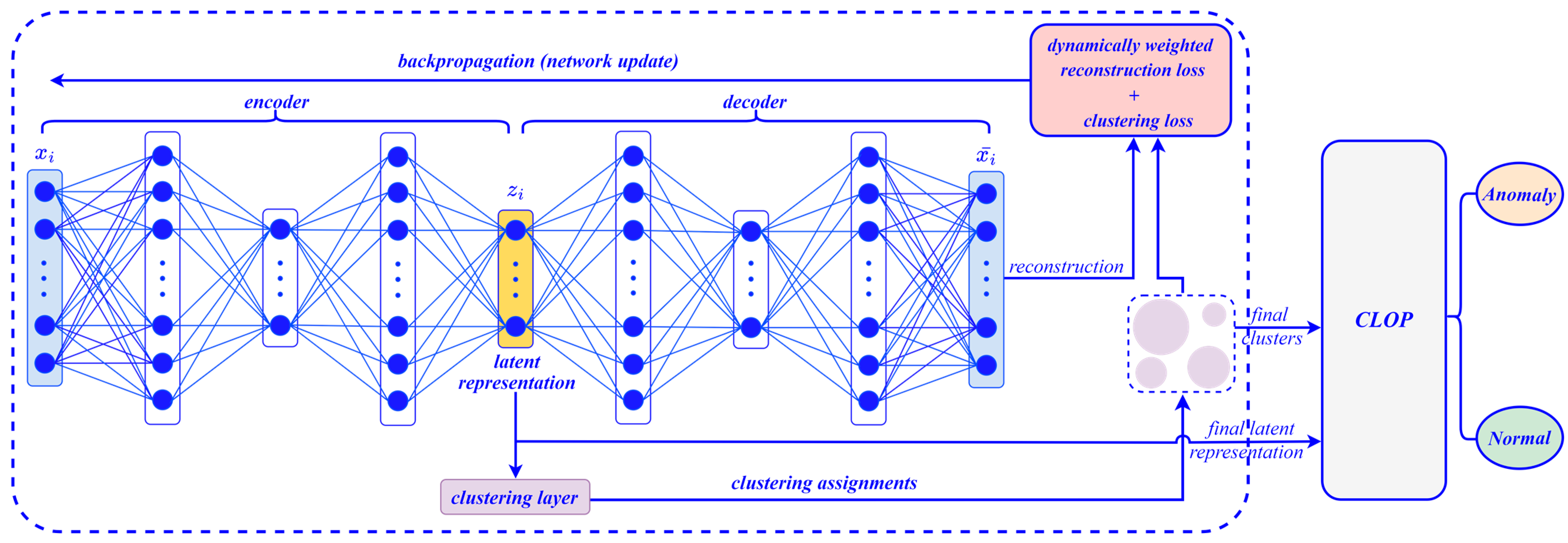
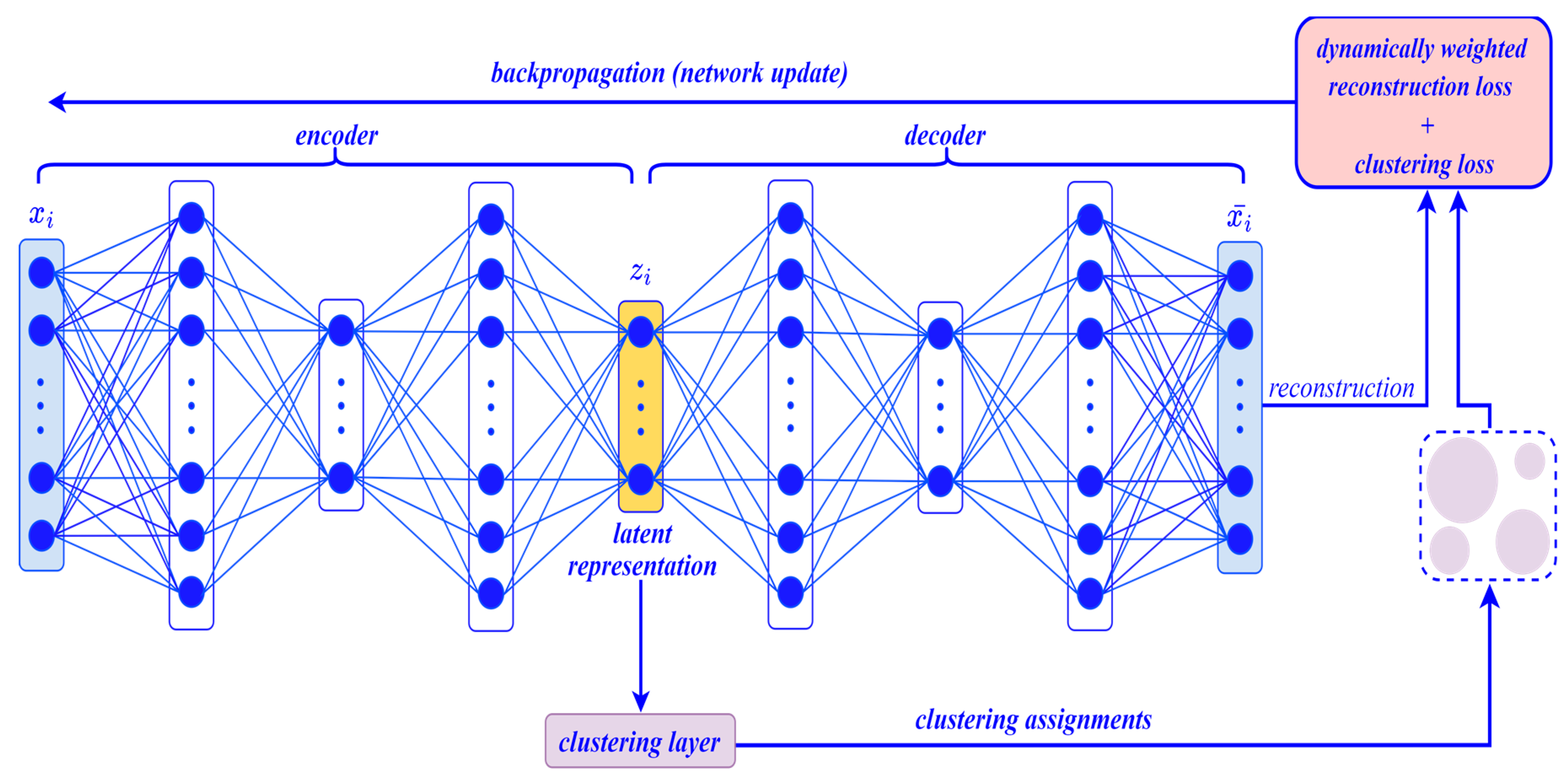
Deep Clustering

Concerning ADCS telemetry data, our proposed deep clustering method presents realistic and explainable results as explained below.

(a)

The method successfully distinguishes day observations (collected by day-time windows) from night observations (collected by night-time windows). Based on the number of the clusters (i.e., 7), the method clusters day observations into two clusters and night observations into four clusters, each expresses a real state of the skCube. By studying the data, we found that the ‘Sun Irradiation’ parameter which is used to detect solar irradiance is the most contributive parameter in distinguishing day observations from night observations. The ‘Sun Irradiation’ parameter includes six irradiation sensors. Five sensors effectively contribute in five separate clusters (as explained below), while the sixth one has 0 irradiance at all times.

▪

Day-time windows: two clusters

(1)

Cluster 1: The most contributive sensor to this cluster is ‘SUN X+ IRRAD’; the high irradiance measured by this sensor is the most significant feature of this cluster.

(2)

Cluster 2: The most contributive sensor to this cluster is ‘SUN Y+ IRRAD’; the high irradiance measured by this sensor is the most significant feature of this cluster.

▪

Night-time windows: four clusters

(1)

Cluster 3: The most contributive sensor to this cluster is ‘SUN X− IRRAD’; the high irradiance measured by this sensor is the most significant feature of this cluster.

(2)

Cluster 4: The most contributive sensor to this cluster is ‘SUN Y− IRRAD’; the high irradiance measured by this sensor is the most significant feature of this cluster.

(3)

Cluster 5: The most contributive sensor to this cluster is ‘SUN Z+ IRRAD’; the high irradiance measured by this sensor is the most significant feature of this cluster.

(4)

Cluster 6: The most contributive sensors to this cluster are ‘SUN X+ IRRAD’ and ‘SUN Z+ IRRAD’; the zero irradiance measured by these two sensors is the most significant feature of this cluster; whereas the irradiance measured by the other ones fluctuated between zero and small irradiance.

(b)

The model successfully gathers the point anomalies and rare events (discussed in Section 5.2.2) into one cluster (the seventh one). This cluster which contains 11 observations is shown in Figure 5 in green.

We conclude that all credit for succeeding in clustering ADCS telemetry data into these realistic and reasonable clusters is ascribed to the fact that our proposed model has effectively learned powerful latent representations and non-linear mappings that allow transforming ADCS telemetry data into a more clustering-friendly representation. Therefore, the method is able to efficiently cluster ADCS telemetry data into significant and explainable clusters, each expressing a real state of the skCube. We believe that the detection of these patterns provides engineers with valuable information that helps them better monitor the state of the satellite and use it as a ground truth for comparing it with the corresponding upcoming telemetry packets.

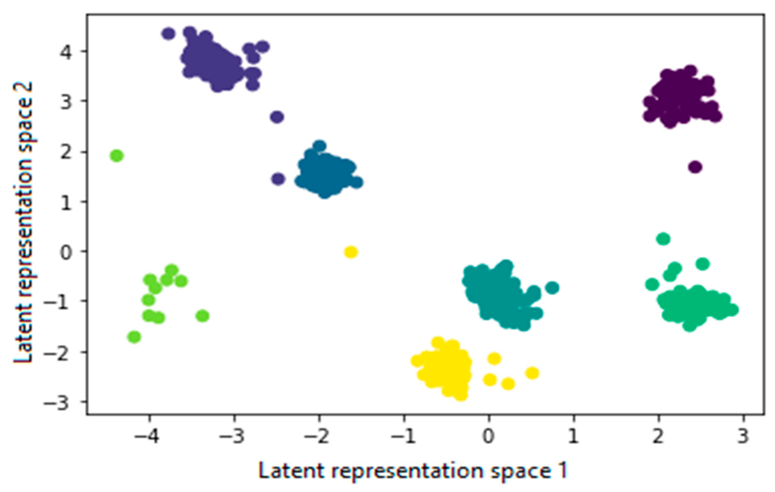
Figure 5 shows the result of the deep clustering model in two-dimensional space from the seven latent representation spaces. As shown in the depicted figure, all clusters are well separated; the two clusters of day observations are on the upper left corner, the four clusters of night observations are on the right side, while the seventh cluster containing anomalies and rare events is in green color on the lower left corner.

Figure 5. Result of deep clustering.

Figure 5. Result of deep clustering.

• Case Study 1: Normal Operation (day and night-time windows)

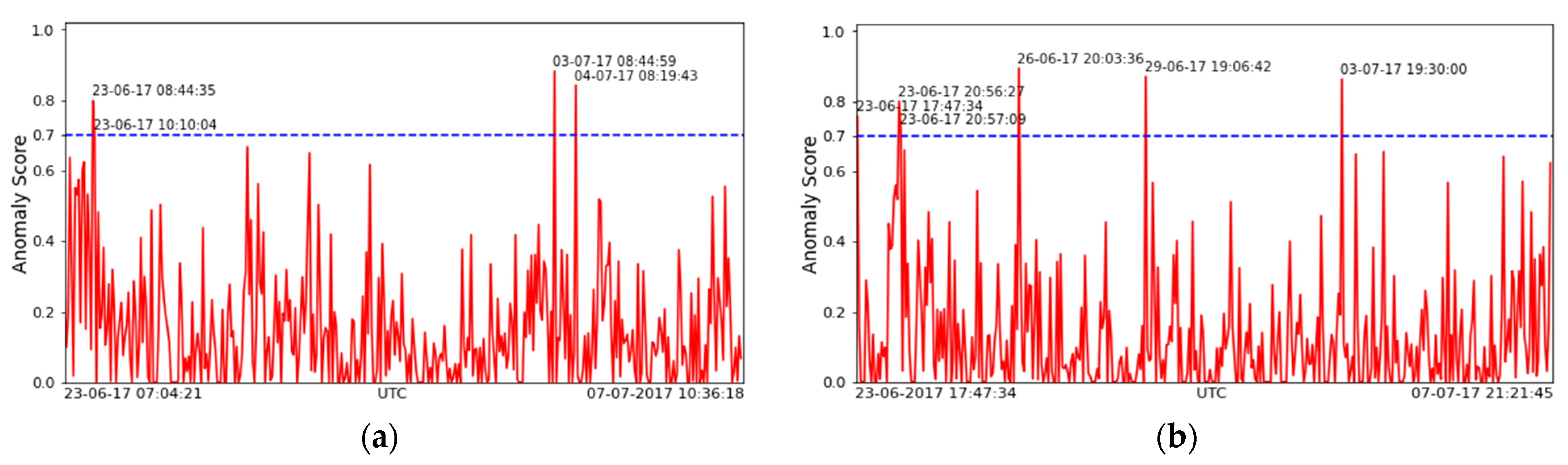
The CLOP anomaly score of these six clusters most frequently remains within the range of 0 to 0.7 in general. Therefore, we choose an anomaly score value of 0.7 to be our threshold. The observations with anomaly scores higher than the threshold (i.e., 0.7) are repeated four times only in clusters that represent day observations, and six times only in clusters that represent night observations. We conclude that the increase in the anomaly score of these observations is definitely a false alarm as the skCube operators did not report any symptoms of abnormal behaviors for such observations. Figure 6 shows the CLOP anomaly score for the above-mentioned normal period operation.

2.

Case Study 2: Anomalous and Rare Events (Magnetometer Events)

The aforementioned point anomalies and rare events are represented by one cluster in which the model collects only 11 observations. The collected observations represent one rare and ten unusual measurements of the two magnetometers. These measurements may occur due to an error in the monitored value, an error in the sending packet, an error in converting the sending packet, or a real value. In all cases, the model should detect these unusual measurements regardless of the reason why they rise. The detected observations in this cluster are discussed and explained below.

i.

Rare Measurement of Magnetometer

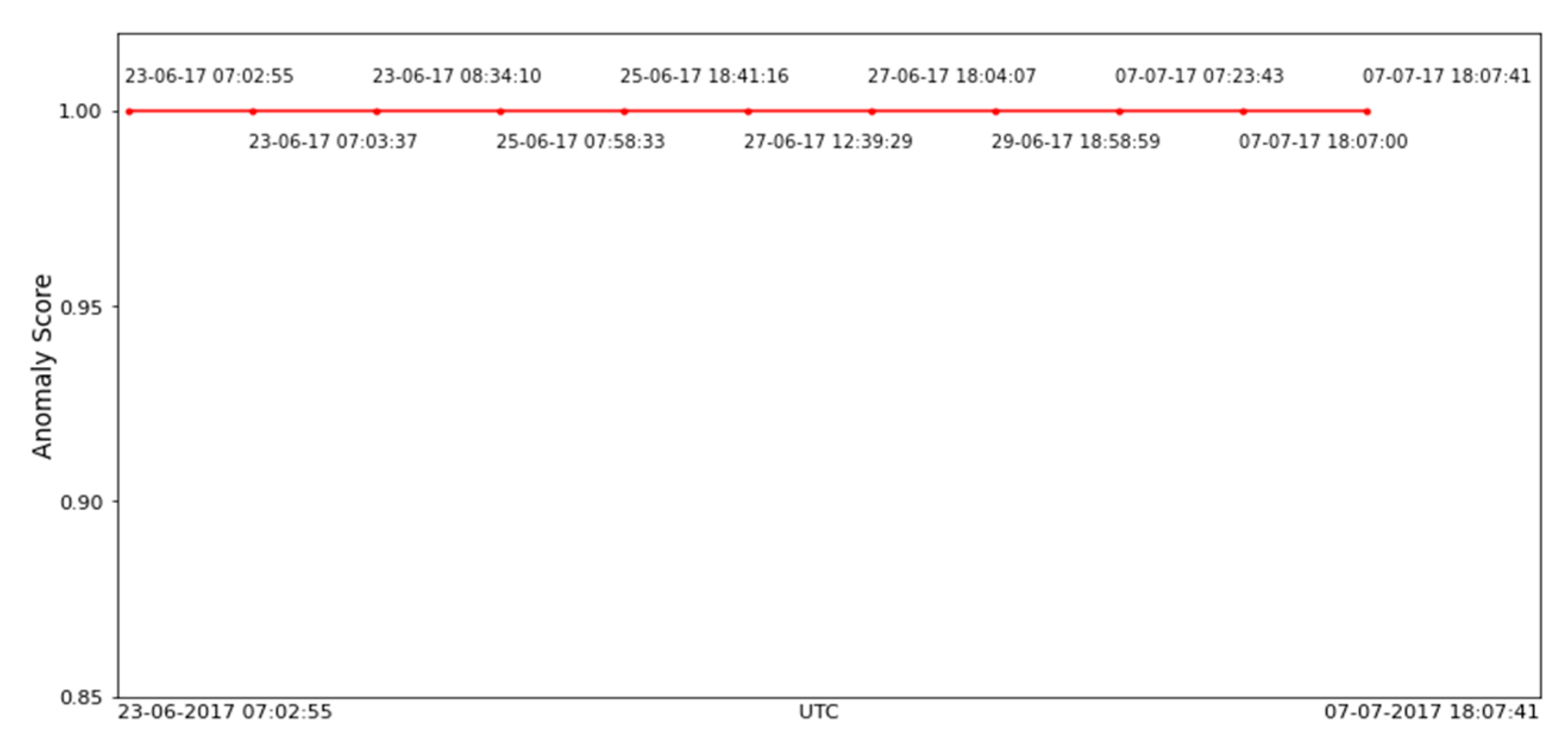
The model successfully detects the aforementioned rare event and puts it into a separate cluster (the green one in Figure 5) together with the other point anomalies explained below. Figure 7 shows that the CLOP anomaly score of this rare observation is of the value of 1.0 (the maximum value of CLOP score).

ii.

Zero Measurement of Magnetometer

The model successfully detects all these 10 observations as point anomalies and puts them together into one cluster (the green one in Figure 5). Figure 7 shows that the CLOP anomaly scores of these point anomalies (five to the right and five to the left of the above-mentioned rare event) are of the value of 1.0 (the maximum value of CLOP score). The CLOP anomaly scores are the highest among all other anomaly scores of the observations of the normal operation.

Figure 7. CLOP anomaly score of anomalies and rare events.

Figure 7. CLOP anomaly score of anomalies and rare events.

▪

Evaluation Metrics and Comparison

The evaluation of our proposed DCLOP is two-fold. The first one is the evaluation and analysis of the quality of the proposed clustering method using unsupervised metrics. The second one is the evaluation of the proposed DCLOP as an anomaly detection method. Although the ADCS telemetry data, which is transmitted from a live skCube satellite, is unlabeled, we managed to create a ground truth using the study discussed in Section 5.2.2. Based on this ground truth, ADCS telemetry data contains (i) 782 nominal observations (382 day observations and 400 night observations) and (ii) 11 point anomalies and rare events.

i.

Deep Clustering Evaluation

The clustering of normal operational data into day and night observations is one major concern of this paper. From the perspective of the day- and night-time windows, this clustering operation can be considered a binary clustering problem and can consequently be evaluated using performance metrics of the binary classification confusion matrix [37].

The evaluation measures are reported in the form of a confusion matrix as shown in

Table 1. Confusion matrix of clustering normal telemetry data evaluation measures.

		Predicted
		Day	Night
Actual	Day	TP	FN
	Night	FP	TN

, where TP represents day observations that are clustered correctly, while FN represents day observations that are clustered incorrectly. For night observations, TN represents night observations that are clustered correctly, while FP represents night observations that are clustered incorrectly.

Based on the confusion matrix, the standard performance measures [38,39] can be defined and calculated to evaluate the performance of the deep clustering method. Since the deep clustering results are not deterministic, the performance measures of anomaly detection have been averaged over 10 runs.

Regarding the clustering performance measures,

Table 2. Deep clustering performance evaluation results for DCLOP.

	DCLOP + Static Loss	DCLOP + Adapted Dynamically Weighted Loss
Accuracy	96.42%	97.73%
Sensitivity	97.00%	98.10%
Specificity	96.80%	97.40%
Precision	0.957	0.973
$NPV$	0.971	0.982
$F_1$-Score	0.963	0.976
FPR	0.039	0.025
FNR	0.027	0.018
MCC	0.933	0.955

reveals that the deep clustering method (in DCLOP) with dynamically weighted loss achieved slightly higher performance measures in all the evaluation measures when compared to the one with static loss.

On the other hand, the clustering quality is evaluated using the following three unsupervised metrics: (i) silhouette score [40], (ii) Calinski–Harabasz Index [41], and (iii) Davies–Bouldin Index [42].

According to the clustering evaluation metrics,

Table 3. Deep clustering evaluation.

	Silhouette Score	CH Index	DB Index
DCLOP + static loss	0.746	2275.592	0.361
DCLOP + dynamically weighted loss	0.824	4311.016	0.253

reveals that the deep clustering method (in DCLOP) with dynamically weighted loss had better performance on all the 3 metrics when compared to the one with static loss.

ii.

Anomaly Detection Evaluation

The evaluation measures are reported in the form of a confusion matrix, as shown in

Table 4. Confusion matrix of anomaly detection evaluation measures.

		Detected
		Anomaly	Normal
Actual	Anomaly	TP	FN
	Normal	FP	TN

[37], where TP represents anomalies that are predicted correctly, while FN represents anomalies that are predicted incorrectly. For normal observations, TN represents normal observations that are predicted correctly, while FP represents normal observations that are predicted incorrectly.

The technical challenge ADCS telemetry data poses while predicting anomalies is the highly imbalanced distribution between nominal and anomalous observations. Based on the aforementioned created ground truth, the anomaly percentage in our case is 1.37% (11 out of 793 observations) of the total observations. Choosing appropriate metrics is particularly difficult for such an imbalanced anomaly detection model. This difficulty is attributed to the fact that (i) most of the widely used standard metrics assume a balanced class distribution and (ii) not all classes (and therefore not all prediction errors) are equal for an imbalanced anomaly detection problem. Therefore, additional evaluation metrics that focus on the minority class are required. For this purpose, standard metrics such as sensitivity, specificity, FPR, FNR, and accuracy are used. Evaluation metrics for imbalanced anomaly detection are listed below.

• G-performance [43] is the geometric mean of the percentage of anomalies correctly predicted (TPR, Sensitivity) and the percentage of normal observations correctly predicted (TNR, Specificity).

$$\mathrm{G}-\mathrm{Mean}=\sqrt{\mathrm{Sensitivity}\ast \mathrm{Specificity}}$$

(22)

• Error-rate is the ratio of the total number of incorrect predictions (FN + FP) to the total number of the dataset (P + N). It is also defined as the complement of accuracy.

$$\mathrm{Error}-\mathrm{rate}=\frac{\mathrm{FN}+\mathrm{FP}}{\mathrm{P}+\mathrm{N}}$$

(23)

• Receiver Operating Characteristic (ROC) Curve

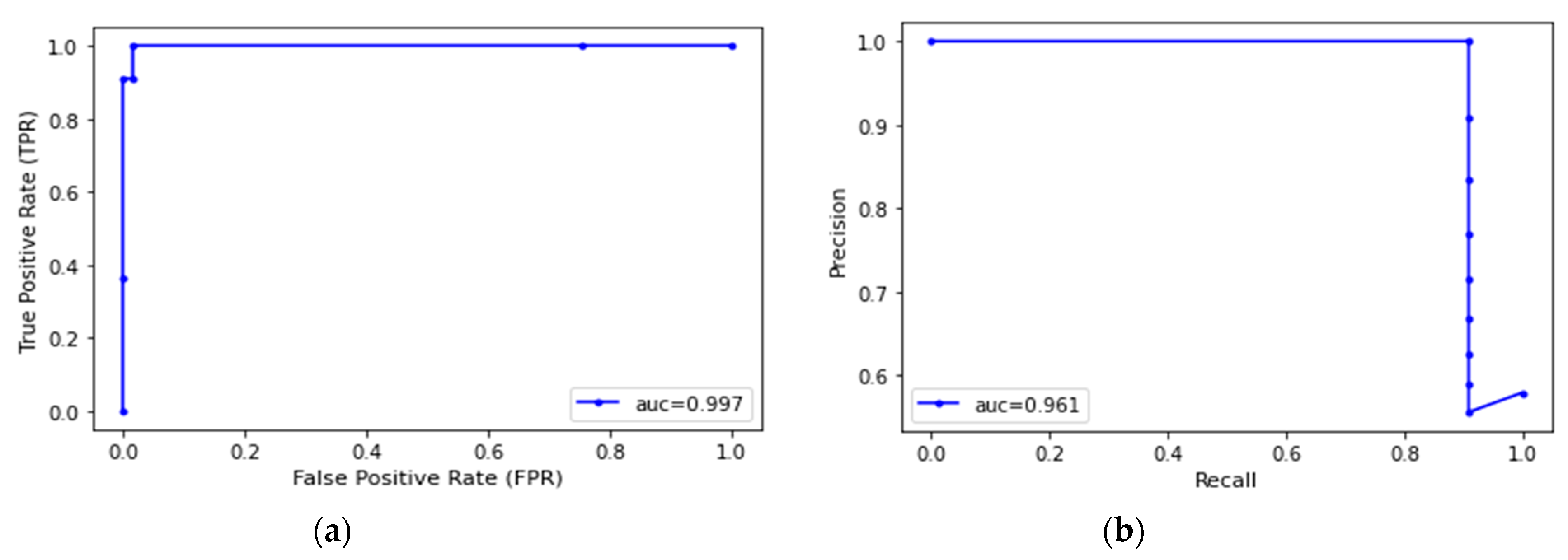
For a better and more qualitative evaluation, the ROC curve is used by varying the outlier threshold [44,45]. The computation is as follows: The true positive rate (TPR) is the proportion of the observations correctly predicted as anomalies to the total number of anomalous observations. The false positive rate (TPR) is the proportion of the normal observations incorrectly predicted as anomalies to the total number of normal observations. These proportions are both in the range of [0.0, 1.0] and are plotted against each other to get the ROC curve. The area under the ROC curve (Auroc) can be computed as another quality measure to evaluate the proposed DCLOP. Figure 8a shows the ROC curve of the DCLOP approach with an AUC score of 0.997.

• Precision-Recall (PR) Curve

The PR curve shows the trade-off between precision and recall. The PR curve is an alternative to the ROC curve and can be used in a similar way. However, it focuses on the performance of the detector on the minority class; this makes it more useful for our imbalanced anomaly detection problem. The area under the PR curve (Auprc) can be computed as another quality measure to evaluate the proposed DCLOP. Figure 8b shows the PR curve of the DCLOP approach with an AUC score of 0.961.

Figure 8. ROC and PR curves of the DCLOP approach. (a) ROC curve; (b) PR curve.

Figure 8. ROC and PR curves of the DCLOP approach. (a) ROC curve; (b) PR curve.

Since DCLOP is based on deep clustering results which are not deterministic, the performance measures of anomaly detection have been averaged over 10 runs.

According to the anomaly detection DCLOP performance measures,

Table 5. Anomaly detection performance evaluation results for DCLOP.

	DCLOP + Static Loss	DCLOP + Adapted Dynamically Weighted Loss
Accuracy	96.99%	98.10%
Sensitivity (TPR)	94.84%	96.40%
Specificity (TNR)	96.98%	98.05%
G-Mean	95.90%	97.20%
Error-rate	0.066	0.018
Precision	0.348	0.420
$\mathrm{NPV}$	0.989	0.999
$F_1$-Score	0.501	0.602
FPR	0.035	0.018
FNR	0.090	0.036
MCC	0.551	0.641
Auroc	0.983	0.997
Auprc	0.948	0.961

reveals that DCLOP with dynamically weighted loss achieved slightly higher performance measures on all the evaluation measures when compared to the one with static loss. The low values of Precision, $F_1$-Score, and MCC are due to the high imbalance in the used telemetry data.

6. Conclusions

This paper contributes to health monitoring in aerospace systems that require early anomaly detection and on-orbit failure warning to identify unusual events, abnormal behaviors, or unexpected measurements. In this paper, we proposed DCLOP, a deep learning approach used for detecting such anomalies and abnormal events. We described the various steps of the approach including data preprocessing, hyperparameter settings, deep clustering in great detail, and anomaly score computation in order to determine nominal and abnormal processes. The contributions of this paper are as follows: A new deep clustering method is proposed based on embedded autoencoder and joint dynamically weighted loss. CLOP is adapted to work on the result of deep clustering method and latent representations in order to compute anomaly score for each observation in telemetry data. The evaluation of the proposed DCLOP approach was conducted on ADCS telemetry data of the skCube satellite. The proposed DCLOP approach is proven to be suitable for analyzing spacecraft housekeeping telemetry data that is high-dimensional and heterogeneous. The experimental results demonstrated that the proposed DCLOP is significantly effective, feasible, and valid in reasonably clustering high-dimensional satellite telemetry data, and also in detecting anomalies inherent. This deep clustering method has been proven efficient in classifying the telemetry data into day-time window observations and night-time window observations. Furthermore, the experimental results demonstrated that DCLOP with the dynamically weighted loss performs slightly better than the one with the static loss. Finally, the promising results of the proposed DCLOP provide satellite engineers with valuable information that might help them monitor the health status of the satellite and consequently hopefully identify the possible causes of anomalies. In addition, the proposed DCLOP shows great promise to be generalized and used for large and complex aerospace systems. In future work, we plan to include the modes and real-time aspects of satellite telemetry. In addition, we plan to propose and use further dynamically weighted loss functions to evaluate them in future models. Furthermore, a general-purpose monitoring system for satellites based on lessons learned in this study shall be addressed.