State of the Art on Two-Phase Non-Miscible Liquid/Gas Flow Transport Analysis in Radial Centrifugal Pumps-Part A: General Considerations on Two-Phase Liquid/Gas Flows in Centrifugal Pumps

Abstract

Gas–liquid mixtures are present in numerous industrial applications, such as in the process industry, oil production and transport with natural gas, deep-sea extraction, and irrigation. Any pump may have to carry multiphase flows. However, the present document is related to non-miscible liquid/gas flow transport analysis in centrifugal pumps because which topic can be a more challenging task compared with axial and mixed flow machines due to specific body force and buoyancy actions and large density differences between the phases. The present document first introduces the main usual gas–liquid two-phase definitions and simplifications. A dimensional analysis introduces the main flow variables and parameters that are used for pumps. Basic physical aspects of flow motion in an impeller channel are explained, and a rapid description of two-phase flow patterns in radial flow pumps is described. Finally, a review of simplified empirical and semi-empirical analytical models is proposed with their limitations.

1. Introduction

The capability of pumps to convey a two-phase mixture depends, in the first place, on whether gas and liquid form a homogenous mixture or to what extent the two phases separate. Fine gas bubbles dispersed in a liquid can be considered as a quasi-homogenous mixture. The bubbles are supposed to be entrained by the liquid flow, but there is some slip between the phases, which may cause additional losses.

However, in a straight channel, pressure gradients in the flow direction are usually moderate, and the pressure field in a rotating impeller strongly influences the phase distribution. A gas bubble always moves in a pressure field to the location of the lowest pressure. Transporting mixtures with high fractions of gas by pumps is a challenging task since gas and liquid tend to separate because of their large density differences. This can be very inefficient or even impossible when phase separation is re-enforced due to intense pressure gradients perpendicular to the main flow direction, such as in centrifugal machines compared with axial ones. Depending on the inlet shape impeller design (e.g., purely two radial blades or 3D blade shapes), different phase velocities occur close to the suction surface region at the impeller inducer part. Because a negative pressure gradient prevails, the bubbles move more quickly than the water. Thus, in the space just after this region, the distributions of the void fraction obtained are higher and uneven. The change in the pressure distribution owing to air admission is also particularly evident in the inlet region of the impeller. These changes bring about an alteration of the whole flow pattern in the impeller and cause a drop in pump performance. With larger gas volume fractions, bubbly flow is no longer possible since small bubbles tend to coalesce to form larger gas accumulations (as in slug or plug flow in a pipe). When gas accumulates in the pump, the delivery can be disrupted, and the pump becomes “gas-locked”.

Liquid droplets that are transported inside a mainstream gas can also be considered a homogeneous mixture but are not considered here.

2. Two-Phase Parameters for Pump Applications

The parameters that are usually used for pumps are listed below. These parameters are deduced from basic two-phase definitions but with several assumptions. All details are given in Appendix A.1.

• Gas fraction x:

$$\mathrm{x}={\dot{m_G}/(\dot{m}}_G+{\dot{m}}_L), \mathrm{a}\mathrm{s}\mathrm{s}\mathrm{u}\mathrm{m}\mathrm{i}\mathrm{n}\mathrm{g} \mathrm{s}\mathrm{t}\mathrm{e}\mathrm{a}\mathrm{d}\mathrm{y} \mathrm{s}\mathrm{t}\mathrm{a}\mathrm{t}\mathrm{e} \mathrm{c}\mathrm{o}\mathrm{n}\mathrm{d}\mathrm{i}\mathrm{t}\mathrm{i}\mathrm{o}\mathrm{n}.$$

(1)

2.

Void fraction α:

$$\alpha =\frac{Q_G}{Q_G+Q_L}, \mathrm{a}\mathrm{s}\mathrm{s}\mathrm{u}\mathrm{m}\mathrm{i}\mathrm{n}\mathrm{g} \mathrm{s}\mathrm{t}\mathrm{e}\mathrm{a}\mathrm{d}\mathrm{y} \mathrm{s}\mathrm{t}\mathrm{a}\mathrm{t}\mathrm{e} \mathrm{c}\mathrm{o}\mathrm{n}\mathrm{d}\mathrm{i}\mathrm{t}\mathrm{i}\mathrm{o}\mathrm{n}.$$

(2)

3.

Slip ratio between phases S_V:

$$S_V=\frac{V_G}{V_L}$$

$$\mathrm{or}{S}_V=\frac{W_G}{W_L} \mathrm{depending} \mathrm{on} \mathrm{the} \mathrm{absolute} \mathrm{or} \mathrm{relative} \mathrm{frame}.$$

(3)

4.

Mass flux G:

$$G={(\dot{m}}_G+{\dot{m}}_L)/A \mathrm{i}\mathrm{n}(\mathrm{k}\mathrm{g}/\mathrm{s}/\mathrm{m}{}^2)$$

(4)

5.

Homogeneous two-phase density ρ_tp:

$${\rho }_{tp}={\alpha }_V{\rho }_G+\left(1-{\alpha }_V\right){\rho }_L$$

(5)

3. Dimensional Analysis Application in Pumps

When a two-phase gas–liquid mixture is present in any rotating machine, the increase of pressure in the pump Δ$p_{tp}$ can be written as a function of several variables listed below:

-

A characteristic length of the pump, i.e., the impeller diameter d_imp;

-

The rotational speed n;

-

The gas and liquid flow rates, respectively, Q_G and Q_L;

-

The gas and liquid densities ρ_G and ρ_L;

-

The gas and liquid kinematic viscosities υ_G and υ_L;

-

The surface tension σ;

-

The gravitation acceleration.

$$\Delta p_{tp}=F(d_{imp},n,Q_L,Q_G,{\rho }_L,{\rho }_G,{\upsilon }_L,{\upsilon }_G,\sigma ,g)$$

(6)

This suggests that inlet pressure and temperature are not considered here, not because they are not important parameters but because their influences are neglected in the present approach. Therefore, cavitation effects are excluded here, although they effectively belong to the two-phase flow category that also affects pump performances but are governed by different physics.

If one takes $d_{imp}$, $n$ and ${\rho }_L$ (*) as fundamental variables, it is possible to define eight non-dimensional groups and write:

$$\begin{gathered} \begin{array}{l}\Delta p_{tp}/{\rho }_L((n{d_{imp})}^2)=\\ \\ {\mathrm{F}}^{\prime }{Q}_L/\left(n_{}{d}_{imp}^3\right), Q_G/\left(n_{}{d}_{imp}^3\right), {\rho }_{G,}/{\rho }_L, \left(n_{}{d}_{imp}^2\right)/{\upsilon }_L,\left(n_{}{d}_{imp}^2\right)/{\upsilon }_G,\\ \\ {n}^2{d}_{imp}/g,{\rho }_L{n}^2{d}_{imp}^3/{\sigma }_{}\end{array} \end{gathered}$$

(7)

(*) Note that the liquid density appears here instead of the density mixture (that must also be defined). The liquid phase is consequently supposed to be the primary flow that governs the main resulting pressure field in the pump.

-

$n_{}{d}_{imp}^2/{\upsilon }_{G{}^{\mathrm{L}}}$ is related to the liquid phase Reynolds number. Typical values reach 2 × 10⁶, which means that viscous effects are mostly concentrated inside boundary layers. Viscous effects can be neglected compared with inertia terms.

-

$n_{}{d}_{imp}^2/{\upsilon }_G$ is related to the gas phase Reynolds number, and typical values are close to 1 × 10⁵.

-

${\rho }_L{n}^2{d}_{imp}^3/{\sigma }_{}$ is related to the Weber number. Typical values are around 3 × 10⁶. This means that the surface tension effects can be considered negligible compared with liquid inertia effects.

-

$\frac{g}{n^2{d}_{imp}}$ is related to the ratio between gravitation and centrifugal forces, often represented by the Froude number. The order of magnitude is about 5 × 10⁻². The centrifugal acceleration can be considered the most important one compared with the gravitational one inside the rotating parts of the pump.

-

$\frac{{\rho }_G}{{\rho }_L}$ is close to 10⁻³, if an air–water mixture is considered. This suggests that the most important effects on the pressure field are dominated by the liquid phase, as already mentioned. Note that, in some cases, this density ratio may be controlled and may not be neglected.

By taking all the above assumptions and simplifications, one can write:

$$\Delta p{}_{T,tp}/{\rho }_L({(n{d}_{imp})}^2)={\mathrm{F}}^{″}(Q_L/(n_{}{d}_{imp}^3),\frac{{\rho }_G}{{\rho }_L})$$

(8)

For all other terms depending on $\frac{Q_L}{Q_G}$, another variable $\beta =\frac{Q_G}{Q_L}$ is introduced so that:

$${\alpha }_V=\frac{Q_G}{Q_G+Q_L}$$

(9)

$${\alpha }_V\left(1+\frac{1}{\beta }\right)=\frac{\beta }{1+\beta }$$

(10)

Therefore, $\beta =\frac{{\alpha }_V}{1-{\alpha }_V}$ and $\left(1-{\alpha }_V\right)\left(1+\beta \right)=1$.

Relation (8) can be written as follow:

$$\Delta p_{T,tp}/{\rho }_L((n{d}_{imp}){}^2)={\mathrm{F}}^{‴}((1+\frac{Q_G}{Q_L})\times n{d}_{imp}^3,{\alpha }_V)$$

(11)

or:

$$\Delta p_{T,tp}/{\rho }_{tp}((n{d}_{imp}){}^2)={\mathrm{F}}^{‴}((1+\frac{Q_G}{Q_L})\times Q_{L}n{d}_{imp}^3,{\alpha }_V)$$

(12)

$$\mathrm{w}\mathrm{i}\mathrm{t}\mathrm{h} {\rho }_{tp}=\left(1-\alpha \right){\rho }_L+\alpha {\rho }_G$$

(13)

This means that the pressure increase in a pump under two-phase conditions mainly depends on the flow coefficient and the local void fraction.

Note that the local void fraction can change inside the pump, being dependent on the flow coefficient. The separation of the variables that is proposed in this dimensional analysis is thus questionable. In Section 5.1, the method proposed by Mikielewicz for correlating performance characteristics for pumps under two-phase flows leads to the same identification of these two major parameters.

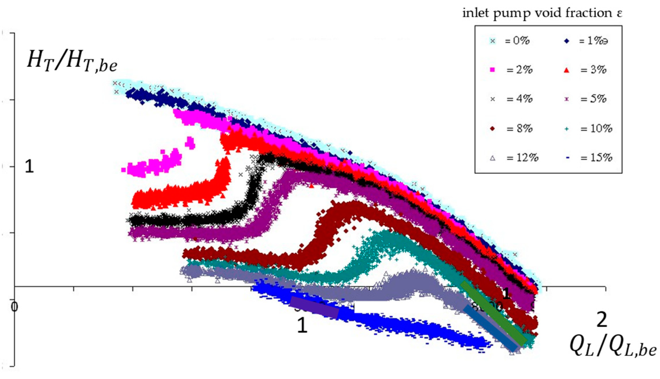
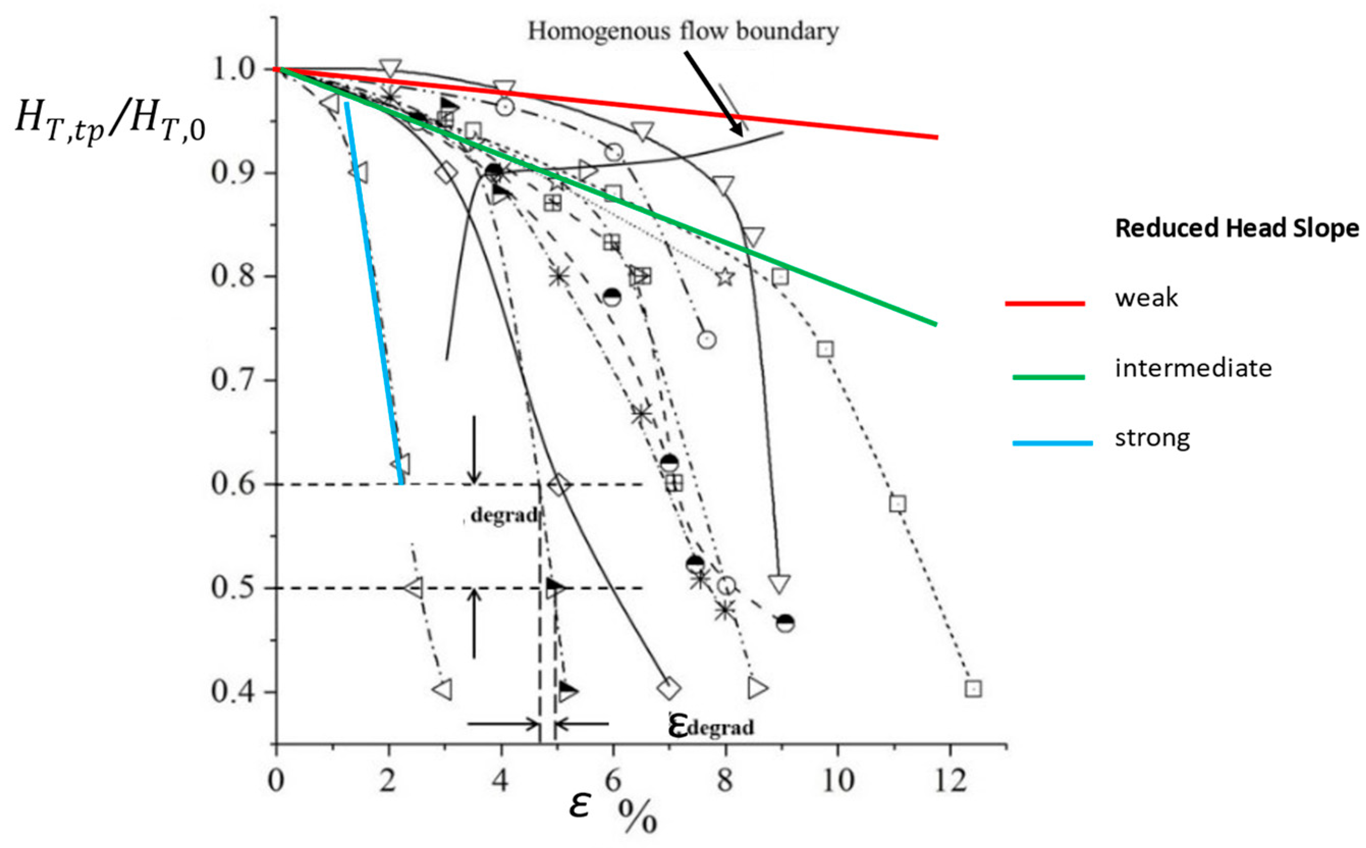
4. Pumps Two-Phase Performance Representation—Basic Physical Aspects

Investigation on two-phase flows in pumps is often compared with single-phase liquid conditions using the inlet pump void fraction ε instead of the local one α, which is generally not known and is a result of how the flow mixture evolves inside each pump fixed or rotating parts.

The total head coefficient ${\psi }_T$ and flow coefficient $\phi$ are introduced as follows:

${\psi }_T=\frac{g{H}_T}{U_2^2}=F^1\left(\phi ,\alpha \right)$, for incompressible flow and iso thermal condition.

or

$${\psi }_T=\frac{g{H}_T}{U_2^2}=F^1\left(\phi ,\epsilon \right)$$

(14)

The pump performance curves usually consider the pump as a «black box».

Figure 1 gives an example of such curves. (Data from Gamboa and Prado [1]). The pump head decreases for increasing inlet void fraction values ε. Pump surging corresponds to the beginning of the sharp head decrease, the location of which depends on the liquid flow rate. Gas lock areas are related to constant head values on the left-hand side.

Depending on the pump design and the operating point, the mean cross-section void fraction α inside the pump is always observed to be higher than the inlet value ε.

The way the liquid flow rate (that is finally delivered by the pump) is changing directly depends on the loss level inside the pump channels, which is also related to the increase in the inlet void fraction. Estevam et al. [2] and Barrios [3] propose the so-called “two-phase mapping” plot (Figure 2) to show how the liquid flow rate can be related to the gas flow rate in association with flow patterns that have been identified by several authors and described in the next section.

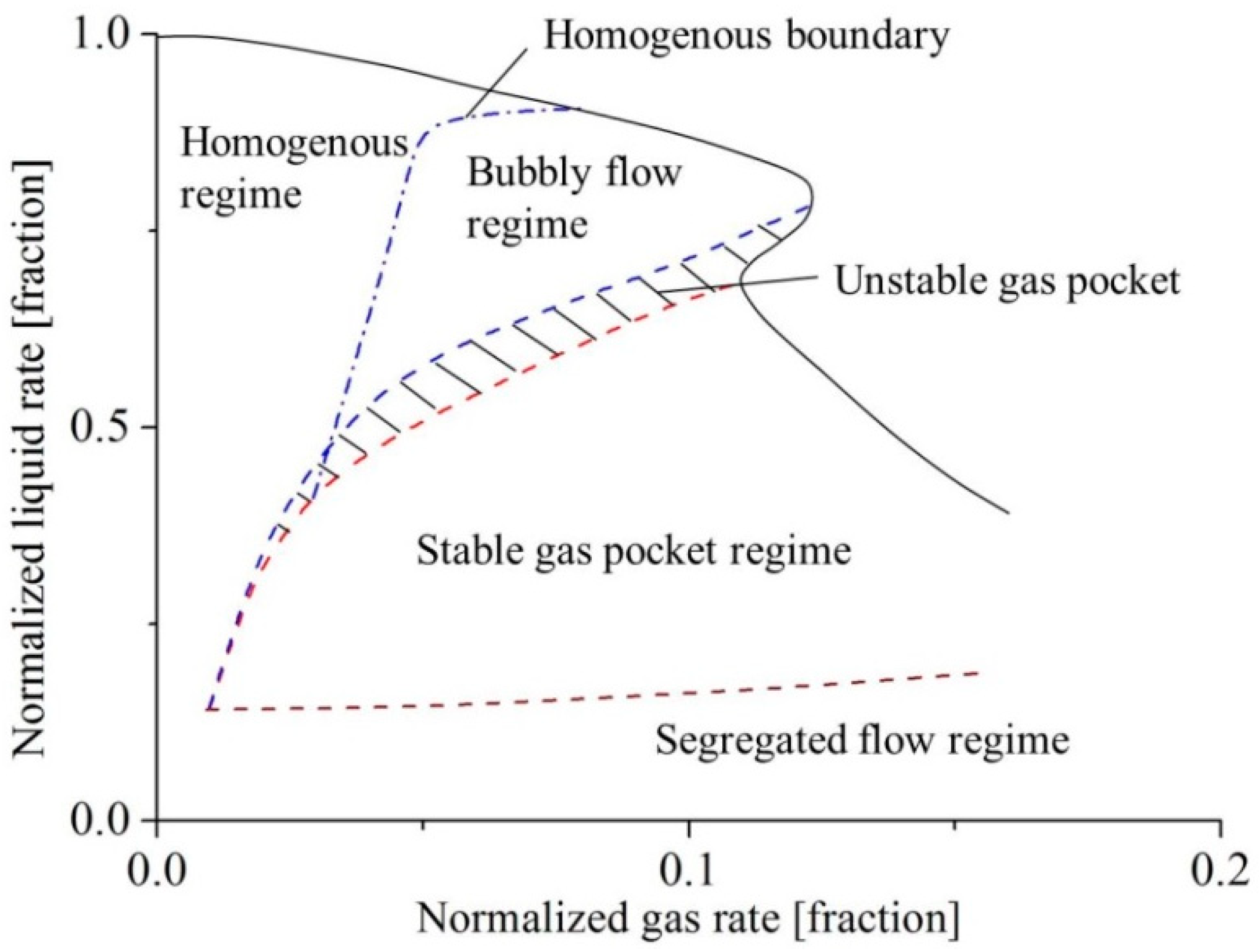
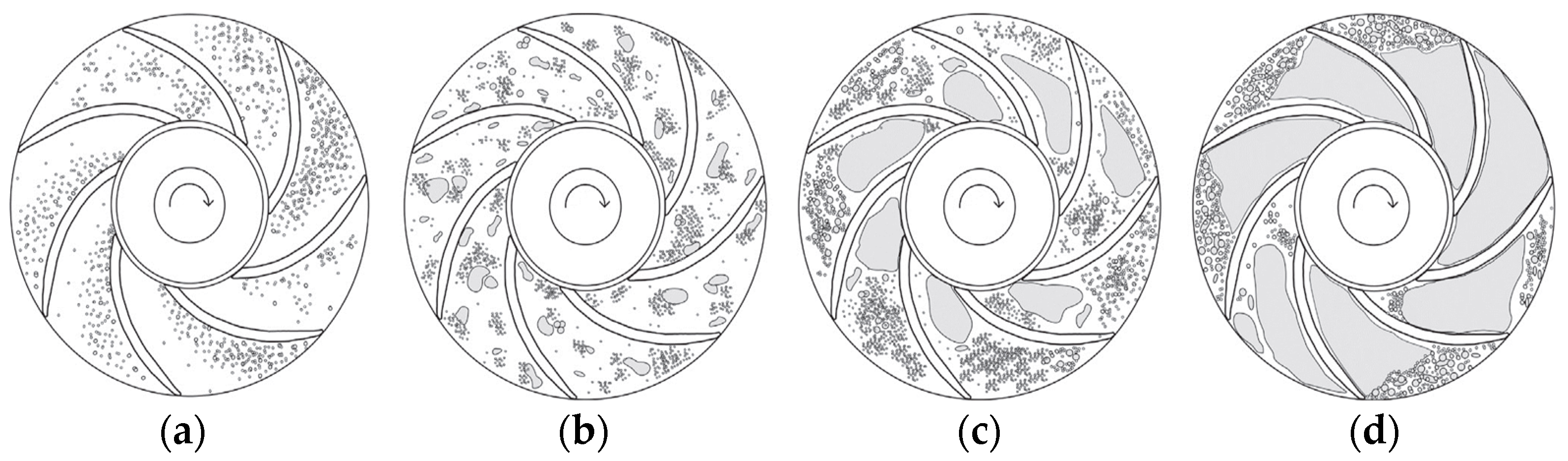
4.1. Two-Phase Flow Patterns Inside a Pump

The description and identification of local flow patterns inside a pump are considered using an analogy with what has been observed in horizontal or vertical pipes (Section 5.2), even if the physical phenomena that act on the main flow in pumps are different for pipes (no rotational effects).

Four different flow patterns are detected. Summarized by Verde et al. [4], the schematic representation of each flow pattern is shown in Figure 3 (increasing inlet void fraction from left to right). For small intake void fraction, the flow regime presents tiny and evenly dispersed bubbles inside impeller channels, as shown in Figure 3a. Under this regime, the bubbles are deemed to move together with the liquid phase also inside the impeller (the slippage between gas and liquid is small).

As the intake void fraction increases, the tiny bubbles are prone to collide and aggregate to form bigger ones. In contrast to the bubbly flow regime, the phase slippage between gas and liquid, corresponding to a bubbly agglomerate regime (shown in Figure 3b), can no longer be neglected. Thus, depending on the intake void fraction, the local void fraction α, under bubbly flow, becomes higher than ε. A further increase in inlet void fraction induces more severe collision and aggregation of bubbles so that large gas pocket forms, including agglomerated bubble flow (Figure 3b), gas pocket flow (Figure 3c) and segregated flow (Figure 3d). The intensity of pump performance degradation is directly influenced by the flow pattern within the impeller. The occurrence of the gas pocket flow pattern is linked to the intensification of the deterioration of pump performance and the appearance of operation instabilities. Moreover, the segregated flow patterns correspond to the most severe performance degradation, which makes the pump incapable of generating pressure.

Each flow pattern can generally be associated with specific modifications of pump performance deterioration in relation to liquid flow rate change. More details can also be found in the review paper by Zhu and Zhang [5].

These deteriorations also depend on pump design, flow rate ratio, rotational speed, and inlet void fraction. Inlet bubble diameter is not considered here. A statistical analysis based on two-phase experimental results performed on several conventional centrifugal pumps close to design conditions (Jiang et al. [6]) gives approximate estimations of the maximum admissible inlet void fraction for which homogenous assumption remains valid inside the impeller. This is illustrated in Figure 4, where three colored straight lines are shown for small, intermediate, and strong head slopes versus inlet void fraction. The first two slopes correspond to a quasi-homogeneous flow pattern inside the impeller channel. Keeping such a pattern up to an inlet void fraction of 7% is only possible for a few cases (3D twisted impeller inlet shapes and high rotational speeds).

A head ratio of 50% is reached for a maximum admissible inlet void fraction ${\epsilon }_{degrad}$ of 11–12% at design conditions, as shown in Figure 4. This can be observed for high rotational speeds (above 2500 rpm) or for large impeller outlet radius R (up to U₂ = 25 m/s). However, for low rotational speeds and 2D blade designs, stronger slope is observed (blue line) corresponding to rapid churn and slug flow patterns inside the impeller or even at the impeller inlet pipe. These cases are only able to pump flow mixtures up to 3 to 5% for the same head degradation level. This is summarized in Figure 5.

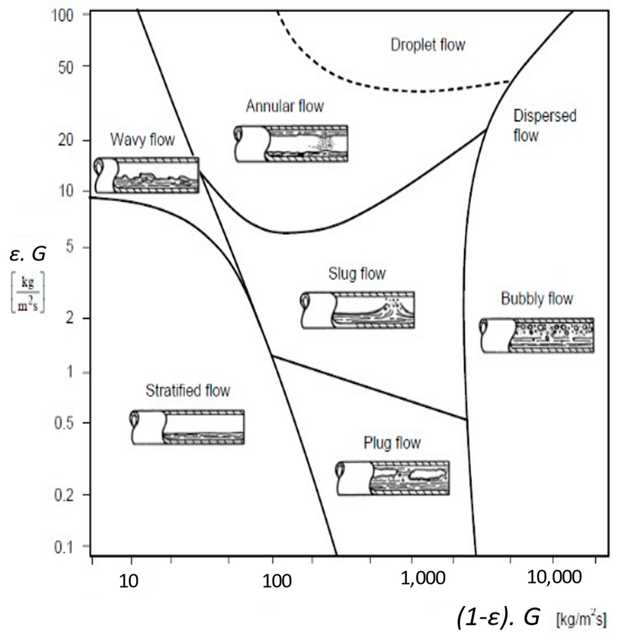
4.2. Analogy with Flow Pattern inside a Tube

The flow pattern observed in Figure 3 is often compared with those found in vertical or horizontal tubes, such as in Figure 6, extracted from Baker [7]. This analogy is purely descriptive, as already pointed out in the previous section. However, such a flow pattern must be detected and well-known at the inlet pipe tube of any pump working under two-phase mixtures, especially when horizontal inlet pipes are used. Depending on the liquid flow rate, the inlet pump flow pattern may not always be a homogeneous bubbly flow regime as frequently supposed or set for inlet boundary conditions.

For a given pump and a given inlet flow coefficient, the flow rate and the head depend on the rotational speed. If, for any purpose, the flow rate becomes lower than the rated one, inlet pipe two-phase flow conditions can jump from a homogeneous bubbly regime to plug or even stratified regimes. Thus, the rotational speed may also have an indirect effect on pump performances due to variable inlet two-phase patterns, as described above. In many experimental results, it is very difficult to distinguish whether the pump performance is affected by non-homogeneous inlet conditions or because of the internal void fraction variation. Shaoa et al. [8] presented an analysis related to this problem, but this is rarely investigated in the open literature.

4.3. Physical Mechanism—Single Phase Conditions

Let us consider the equilibrium of forces acting on a single-phase particle located at point M inside a centrifugal impeller passage. For steady-state conditions, when neglecting shear stresses and momentum exchange between streamlines, the pressure gradient equals the sum of the inertia and centrifugal forces that result from the flow turning plus the centrifugal forces due to both rotation and the Coriolis forces.

This can be expressed on the blade-to-blade plane (see Figure 7) using the streamline coordinates (s, n, b), where s is along the streamline, n is normal to the streamline in the blade-to-blade surface, and b is the binormal perpendicular to s and n:

$$\left(\frac{1}{\rho }\right)\underset{grad}{\to }p=-\underset{W}{\to }\left(\frac{\delta W}{{\delta }_S}\right)·\underset{i_S}{\to }\pm \left(\frac{W^2}{R_b}\right)·\underset{i_n}{\to }+{\omega }^2\underset{R}{\to }-2\omega \underset{W}{\to }\sin \phi ·\underset{i_n}{\to }$$

(15)

The right-hand side terms, respectively, correspond to the streamwise inertia force, the centrifugal force due to the curvature, the centrifugal force and the Coriolis force. The positive sign of the curvature term corresponds to a convex streamline, while the negative sign corresponds to a concave streamline.

Considering backswept blades designs, the radius of the curvature $R_b$ is large, and the Coriolis term is bigger than the centrifugal term. A transverse pressure gradient is generated with the high pressure on the pressure side due to the Coriolis force term.

In the meridional plane shown in Figure 8, where the curvature 1/$R_m$ is large at inlet regions of impellers, while the absolute tangential velocity is small (the tangential velocity component is normal to the meridional plane (Z, R)), a pressure gradient from shroud to hub balances the centrifugal force due to the streamlined meridional curvature. The balance of forces along the normal direction n_m leads to:

$$\frac{\left(\frac{1}{\rho }\right)\Delta p}{\delta n_m}=(V_{\theta }^2/R)\cos \phi -(V_m^2/R_m)$$

(16)

Hence, the inviscid balance of forces leads to a velocity increase from hub to shroud. The impeller flow is controlled by the inviscid forces in the inlet region, where viscous effects are not yet developed. In the radial parts of the impeller, both terms on the right-hand side of Equation (16) will become small and tend to zero.

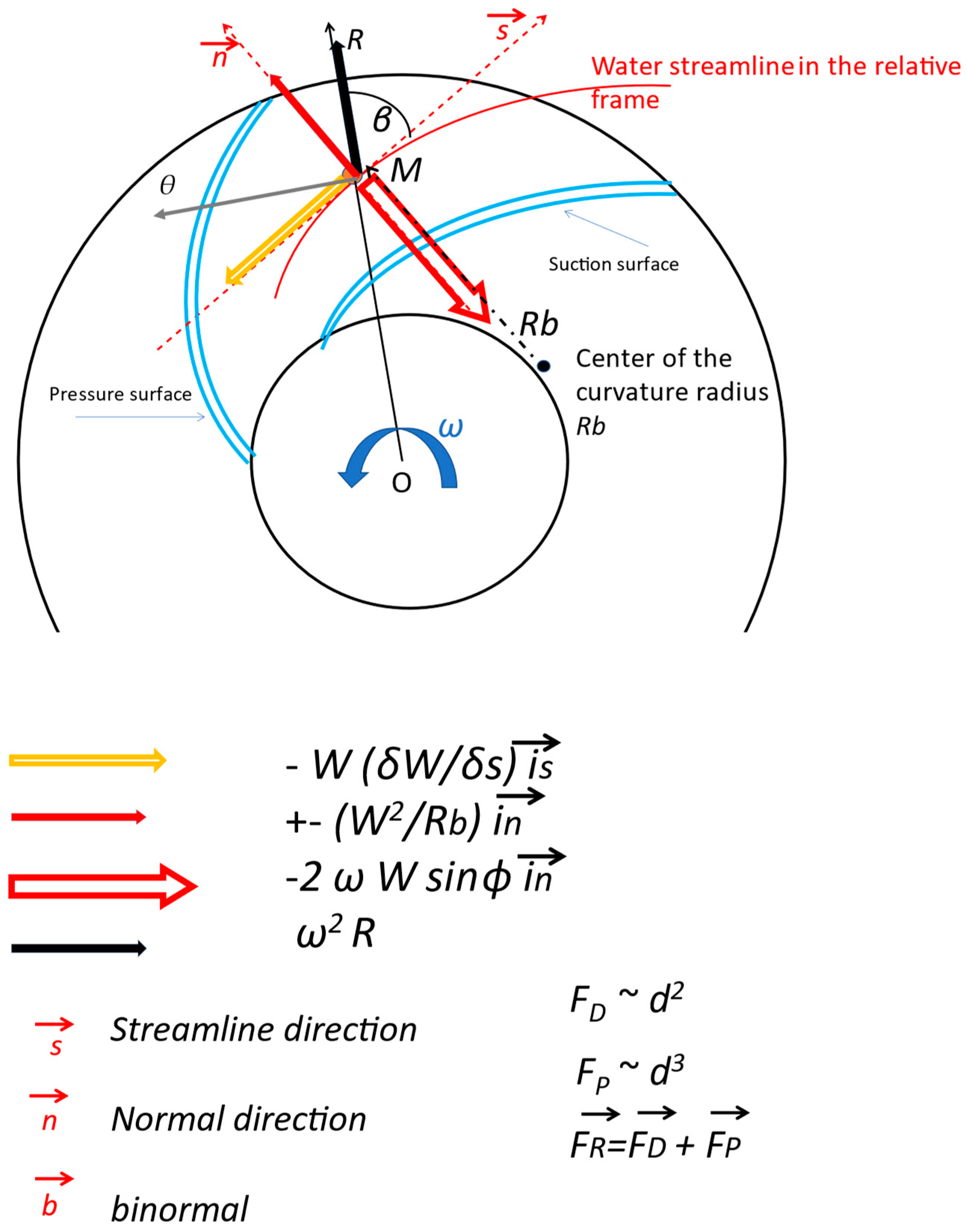
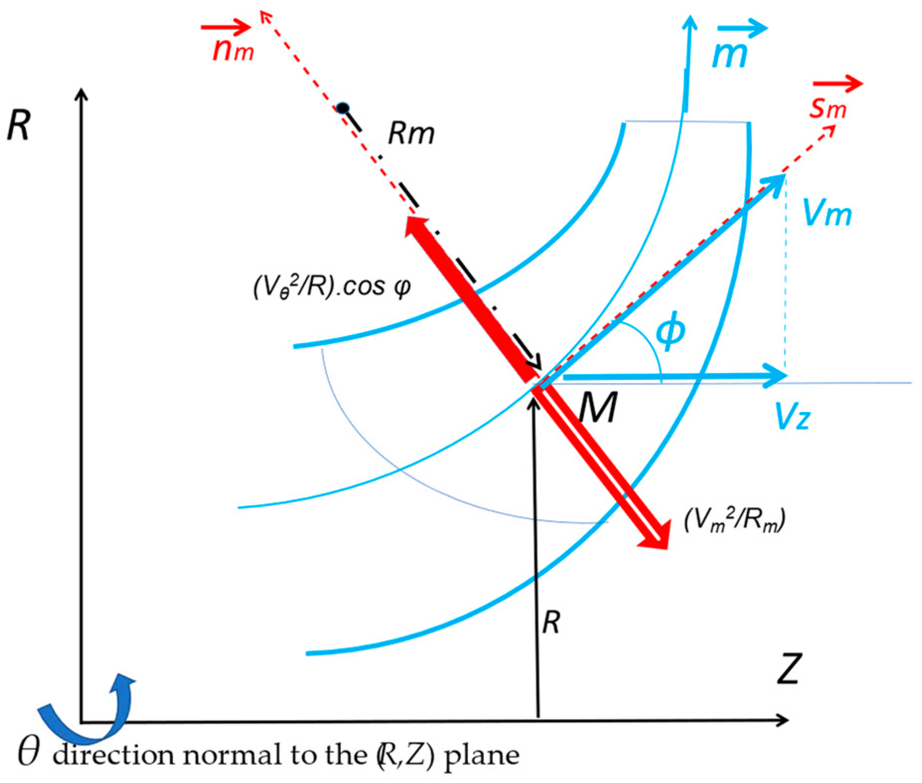
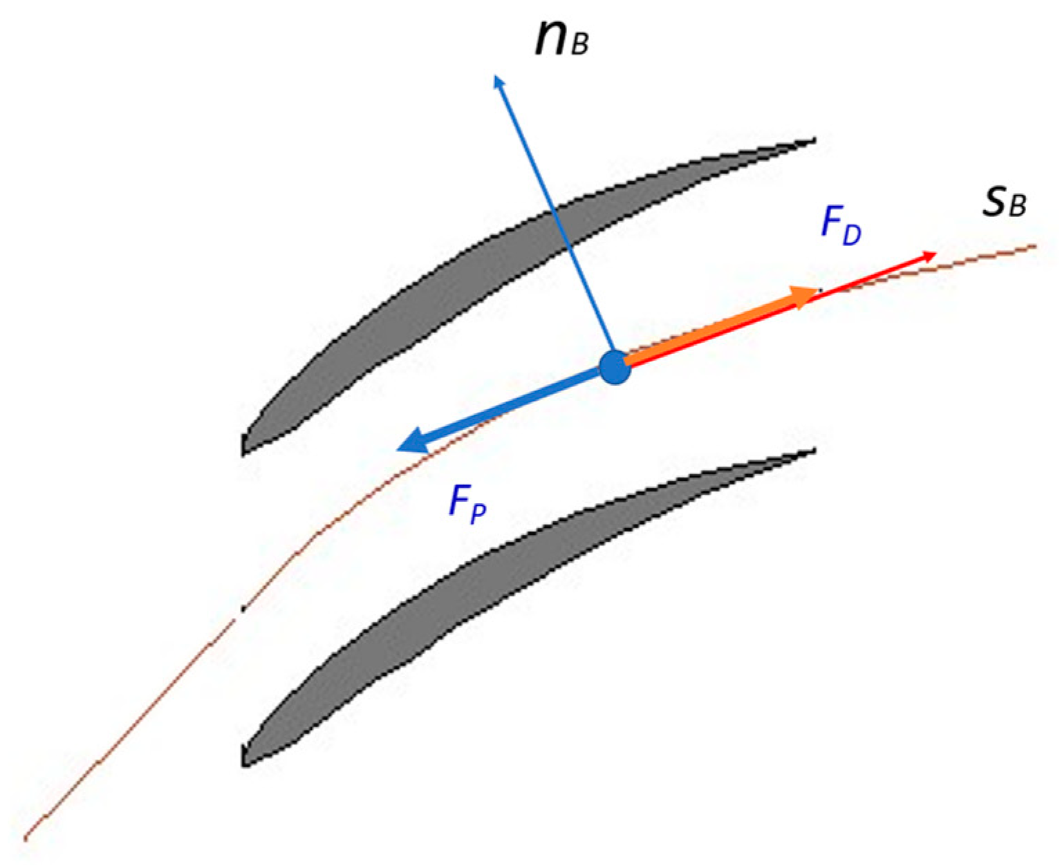
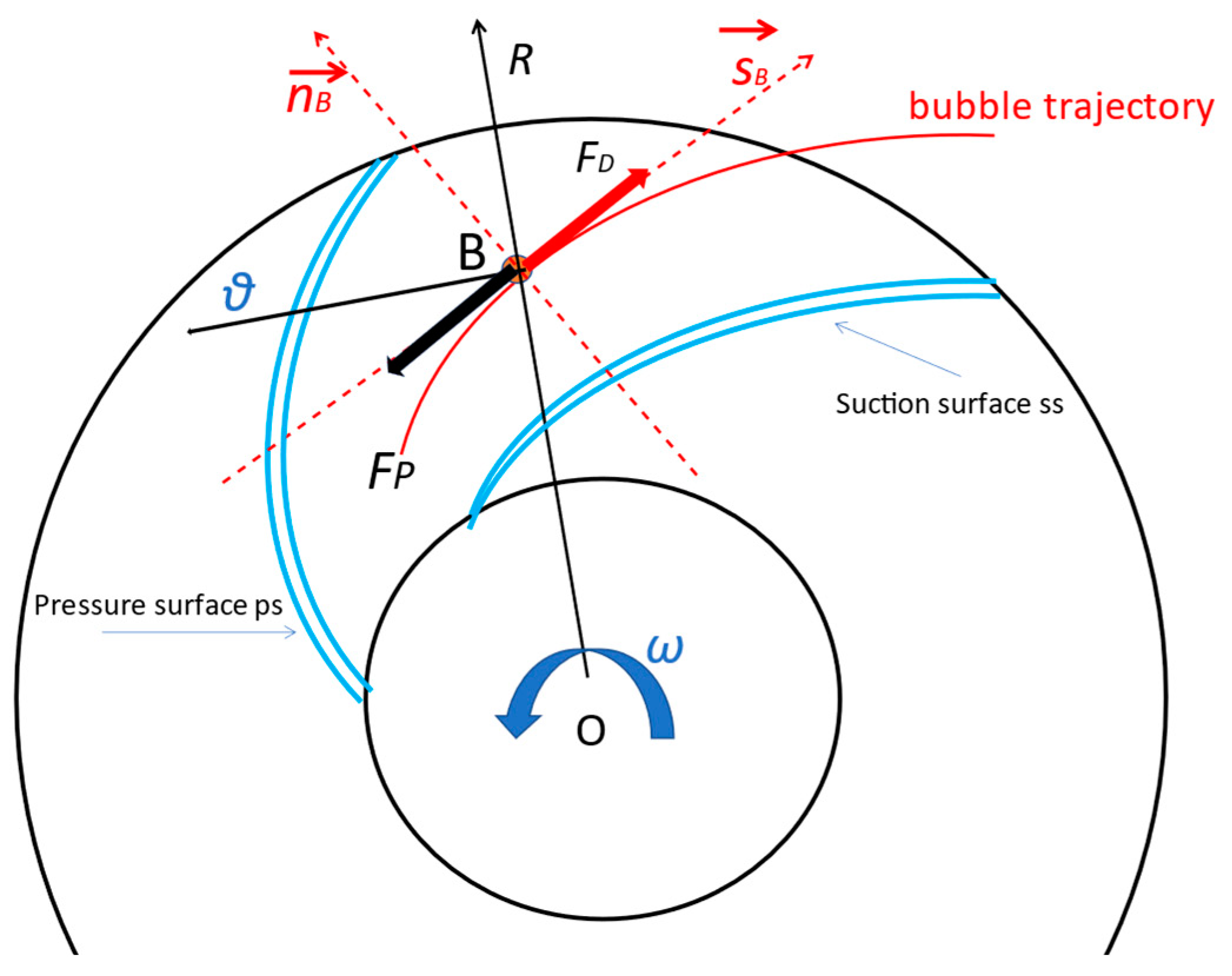
4.4. Physical Mechanism—Forces Acting on a Single Bubble inside the Main Core Flow in an Axial and a Centrifugal Impeller

For an arbitrary pressure field, a gas bubble always tends to be pushed by the main surrounding liquid flow. This result is related to the fluid dynamic drag F_D, which the liquid exerts on the bubble, as shown in Figure 9 and Figure 10.

Assuming that the bubble is mainly affected by the drag force and the pressure gradient force, along with its motion, the force balance on the bubble at a given instant is:

$$\frac{m_B\delta \underset{VB}{\to }}{{\delta }_t}=\underset{FP}{\to }+\underset{FD}{\to }$$

(17)

The left-hand term contains the bubble mass and can be neglected due to the difference between bubble and liquid densities.

Consequently, the velocity of a gas bubble relative to the liquid with a pressure field expressed by the gradient $\frac{\delta p}{\delta s_B}$ can be expressed by the following relation:

$${\left(V_L-V_G\right)}^2-\left(-\frac{\delta p}{\delta s_B}\right)\left(\frac{2d_B}{{\rho }_L}\right)C_D$$

(18)

where $C_D$ is the drag coefficient, and $d_B$ is the bubble diameter. Detailed development can be found in Part C.

In an axial flow impeller passage, the relative velocity deceleration induces less pressure gradient towards the outlet compared with radial machines. A stronger pressure gradient may have an influence when the bubble trajectory departs from its original one. Secondary flows also impact bubble trajectories and velocity change due to the combination of meridional and blade-to-blade curvatures (Gülich [9], chapter 5).

Gas bubble trajectory was experimentally and numerically investigated in a centrifugal impeller by Stel et al. [10] and, more recently, by Ofuchi et al. [11]. Stel et al. [10] found that the bubble trajectories inside the impeller passage are very sensitive to the bubble diameter. When the bubble diameter increases, its trajectory tends to move towards the blade pressure side when leaving the inter-blade second throat area.

Liquid and bubble streamlines also differ depending on the inter-blade location. Other factors, such as rotational speed, flow rate and impeller design parameters, influence bubble trajectories. Bubble deformation has also been observed with larger consequences on drag and trajectories.

However, in real situations, air–liquid mixture contains several bubbles that interact together and make their behavior more complicated. Depending on the flow rate ratio, strong deceleration can occur on the pressure side close to the blade inlet section at a high flow rate. At a low flow rate ratio, strong deceleration occurs on the impeller suction side, generally after the inlet impeller throat area. For both cases, bubbles tend to coalesce together, and a critical gas volume fraction can be reached, creating channel gas blockage and head degradation. Bubble coalescence creates an increase in bubble diameter and/or bubble interactions. The physical analysis performed for a single bubble is no longer valid if phase separation occurs. Momentum exchange between each phase and slip ratio effects must be considered.

Finally, note that the drag force is proportional to the bubble surface, whereas the pressure force is proportional to the bubble volume. If the bubble diameter increases, the pressure force increases faster than the drag force. Each bubble trajectory tendency is thus reinforced.

5. Simplified Approaches for Pumps Two-Phase Performance Prediction

5.1. Semi-Empirical Correlation

Mikielewicz et al. [12] developed a method for correlating pump performance characteristics in two-phase flows producing a “Head- Loss Ratio” which corresponds to the apparent loss of head in a two-phase condition divided by the loss of head in a single-phase condition.

For each phase, Euler equations are developed so that head loss can be extracted from the theoretical head and real one for two-phase conditions.

The theoretical head coefficient obtained with two-phase flow conditions can be written as follows:

$${\psi }_{t,th,tp}=1-f_{tp,2}\phi \tan {\beta }_2 \mathrm{assuming} \mathrm{no} \mathrm{inlet} \mathrm{tangential} \mathrm{absolute} \mathrm{velocity}$$

(19)

Introducing the two-phase function, a:

$$a=\left(\frac{\alpha }{1-\alpha }\right)·\frac{{\rho }_G}{{\rho }_L}$$

(20)

$f_{tp}$ is so defined as:

$$f_{tp}=\frac{\left(1+a\right)\left(1+a{s}_v^2\right)}{1+{a{s}_v}^2}$$

(21)

Note that $f_{tp}=1$, when $s_v=1.$

It is generally assumed that most of the head losses due to two-phase flow patterns mainly occur inside the impeller passage and in the volute but with less extent.

The total two-phase losses are defined as the sum of wall friction losses plus separation flow losses. The separation flow losses can be approximated as being proportional to the square of the actual flow rate $Q_{tp}$ minus the best efficiency one $Q_{be}$.

This leads to the following:

$$\Delta p_{tp,sep}^{LOSS}=K_{sep}{\left\{\left(\frac{Q_L}{{Qtp}_{}}\right)-\left(\frac{Q_{be}}{Q_{tp}}\right)\right\}}^2{Q}_{tp}^2$$

(22)

K_sep is a constant for separated loss correlation that can be obtained or predicted for single-phase conditions.

The expression for the total pressure loss for a given pump can be written as:

$$\Delta p_t^{LOSS}=\Delta p_{t,th,tp}-\Delta p_{t.tp}$$

(23)

which is expressed as the difference between the two-phase theoretical pressure increase in the pump $\Delta p_{t,th,tp}$ and the actual pressure increase $\Delta p_{t,tp}$.

$$\Delta p_t^{LOSS}=f_{sp}\left(\frac{R·L}{A^2}\right)d_{hyd}{\left(\frac{{\rho }_{tp}}{{\rho }_L}\right)}^2{Q}_{tp}^2\left(\frac{{\rho }_L}{2}\right)+K^{\prime }{\left\{\left(\frac{1-\alpha }{1-\alpha +\alpha s_V}\right)-\left(\frac{Q_{be}}{Q_{tp}}\right)\right\}}^2{Q}_{tp}^2$$

(24)

In the above expression, the first term of the second member is directly related to the pressure losses due to wall friction and the second one to separation losses.

-

f_sp corresponds to the usual single-phase friction factor that depends on the pump Reynolds number and the wall roughness factor, as can be found on the well-known Moody diagram.

-

L is an approximated channel length (impeller or volute).

-

A is a characteristic pump area.

-

d_hyd is the hydraulic diameter (impeller or volute).

-

$R={\left(\frac{1-x}{1-\alpha }\right)}^2$

-

$\frac{Q_L}{Q_{be}}=\frac{1-\alpha }{1-\alpha +\alpha s_V}$.

Note that for an air–liquid mixture and for $s_V$ = 1, x is of the order of 10⁻⁴ when α< 30%. Therefore, $R$ can be approximated by $R^{\prime }$$~1/({1-\alpha )}^2$.

This means that the two-phase pressure losses due to friction can be modified by a factor 1/(1 − α)²

For a given pump operating point, let us consider that the two-phase pump head fits the system resistance curve so that:

H_tp = K_sp (Q_G + Q_L)², which suggests that the pump head is only proportional to the square of the total volume flow rate.

Then, it can be approximated by:

H_tp = K_sp (1 + β)² Q_L² = K_sp. Q_L²(1/(1 − α))² = K_spQ_L²R′, which is equivalent to the previous relation except for high void fractions.

The final expression of the Head ratio H*, as proposed by Michielewicz et al. [12], can be written as:

$$\begin{gathered} H^{*}=\frac{\Delta H_{t,tp}^{LOSS}}{\Delta H_{t,sp}^{LOSS}}=\frac{\Delta H_{t,tp,th}-\Delta H_{t,tp}}{\Delta H_{t,sp,th}-\Delta H_{t,sp}}= \\ {(\frac{1+a}{1+as})}^2+K\left\{\left(\frac{1-\alpha }{1-\alpha +\alpha s_V}\right)-{(\frac{Q^{*}}{Q_{tp}})}^2\right\}/\left\{(1-\alpha )(1+a)(1+K{\left(1-\frac{Q_{be}}{Q_{tp}}\right)}^2)\right\} \end{gathered}$$

(25)

In this last relation, K is a combination of the geometrical constant of any one pump and a function of the flow regime, which directly depends on α.

Therefore, $H^{*}$ is principally a function of void fraction and flow coefficient but also a function of rotational speed and slip ratio.

The main assumption about this one-dimensional approach is that each phase enters the rotor with the same absolute angle and leaves the impeller with the same relative angle. It is always possible to verify this assumption, but only when pumping external losses (disk friction and leakage losses) are correctly evaluated from experimental torque measurements (Gülich [9]).

The more homogeneous the flow regime, the more closely the relative losses approach the single-phase values. Therefore, the existence of flow regimes other than homogeneous is the principal determining factor for the prediction of the characteristics in two-phase flow. This includes the problem of loss prediction due to bubble diameter variation, bubble agglomeration and phase separation with associated slip ratio evaluation.

5.2. Analytical Approaches

Analytical approaches have been developed based on one-dimensional hypothesis considering the flow as:

(a)

An average mixture of homogeneous bubbly flow.

(b)

Considering separated phases called the two-phase modeling.

Both approaches lead to solving differential equations allowing for essentially determining the evolution of the local void fraction and slip velocity with flow rate; therefore, it gives more detailed flow features compared with the semi-empirical approach presented earlier.

All detailed development of these methods can be directly found in the related references that are given below. However, the main definitions, assumptions and closure relation that undergo each model are presented in Appendix A.

(a)

One-Dimensional Two-Phase Bubbly Flow Modeling

An analytical method was proposed by Furuya et al. [13] with an inviscid flow assumption to investigate the head degradation due to two-phase pumping. The method is applied in a control volume bounded by two successive streamlines separated by a distance $d_n$, where the momentum equation is developed, then integrated from the impeller inlet to outlet sections assuming that the trajectory of liquid is identical to that of bubbles. A simple interfacial force is introduced using the momentum equation applied to a bubble. The final differential equation is written as follows (see Appendix B):

$$\begin{gathered} {{\dot{(m}}_L}^2/({\rho }_L{d}_n^2))\left(\frac{1}{1-\alpha }\right)\left\{\left(\frac{1}{1-\alpha }\right)\frac{\delta \alpha }{\delta s}-(\frac{1}{d_n})(\frac{\delta d_n}{\delta s})\right\}+{{\dot{(m}}_G}^2/({\rho }_G{d}_n^2))(\left(1-\alpha \right)/{\alpha }^2)\left\{\left(1/\alpha \right)\frac{\delta \alpha }{\delta s}-(\frac{1}{d_n})(\frac{\delta d_n}{\delta s})\right\}+ \\ 0.5{\rho }_L\left\{{{\dot{(m}}_G/{\rho }_G{d}_n\alpha )}^2\left[\left(\frac{1}{\alpha }\right)\frac{\delta \alpha }{\delta s}+(\frac{1}{d_n})(\frac{\delta d_n}{\delta s})\right]\right\}+{{\dot{(m}}_L/{(\rho }_L{d}_n(1-\alpha )))}^2\left[\left(\frac{1}{1-\alpha }\right)\frac{\delta \alpha }{\delta s}-(\frac{1}{d_n})(\frac{\delta d_n}{\delta s})\right]= \\ \left({\rho }_L-{\rho }_G\right)\left(1-\alpha \right)r{\omega }^2\sin \beta \cos \phi \\ -(3/8)(C_D/R_B){\rho }_L\left[{\dot{m}}_L/{(\rho }_L{d}_n(1-\alpha ))-{\dot{(m}}_G/{\rho }_G{d}_n\alpha )\right]\left|{\dot{m}}_L/{(\rho }_L{d}_n(1-\alpha ))-{\dot{(m}}_G/{\rho }_G{d}_n\alpha )\right| \end{gathered}$$

(26)

With the following mass conservation equations:

$${\dot{m}}_{tp}={(\dot{m}}_G+{\dot{m}}_L)$$

$${\dot{m}}_{tp}=d_n\left(1-\alpha \right)W_L{\rho }_{tp}$$

$${\dot{m}}_L=d_n\left(1-\alpha \right)W_L{\rho }_L$$

$${\dot{m}}_G=d_n\alpha W_G{\rho }_G$$

This differential equation contains only one variable α. All other quantities here are either constant or known as a function of s. Therefore, if the boundary conditions at the impeller inlet section are known, the ordinary differential Equation (26) can be solved for α along s. Once α(s) is obtained, all other parameters can be solved. Furthermore, each phase’s relative velocity is determined from the mass conservation equations.

The comparison with experimental data proposed by Furuya et al. [13] shows that head degradation is mainly caused by a higher acceleration in the liquid phase and deceleration in the gas phase than in the case of single-phase flows. Because no relative outlet deviation angle model is proposed (neither slip factor), the results only appear valid when bubbles remain in the main core flow (or close to the suction side of the impeller), which corresponds to flow patterns observed in axial and mixed flow machines.

(b)

One-Dimensional Two-Fluid Modeling (Minemura et al. [14])

This approach is like the one proposed by Furuya et al. [13] but introduces analytical functions for wall friction losses, shock losses, rapid expansion, mixing losses at the impeller outlet on one side, and slip coefficient on another side to determine the effective absolute tangential velocity used for theoretical head evaluation. It is so potentially more applicable to centrifugal pumps.

In addition, several models for interfacial friction coefficient and virtual mass coefficient are proposed and further adapted when applied in real cases.

The constitutive equations allow for calculating the effective performance change operating under two-phase flow conditions using the velocities and void fractions calculated under bubbly flow with slippage between the two phases. It is demonstrated that the head is scarcely affected by bubble diameter in the impeller and friction factor between the two phases for a reduced range of void fraction (α below 25%), whereas it was more affected by the outlet relative velocity differences using the Furuya’s approach but for a wider range of α.

Minemura et al. [14] also presented the results of their model, looking at the evolution of the main parameters along the impeller passage of a centrifugal pump. The following Figure 11 and Figure 12 give interesting comprehension of what should locally occur on the slip ratio, head coefficient and void fraction inside the impeller, such as in Figure 11 (for best efficiency point), and dimensionless loss variations versus inlet void fraction for two different flow coefficients, such as in Figure 12.

In Figure 11, the void fraction reaches maximum values after the impeller’s first throat area and remains almost constant (about three times the inlet value). A significant increase can be detected when the inlet void fraction ε is bigger than 0.06. A rapid decrease of the velocity ratio is also observed and corresponds to the increase of the head loss coefficient.

In Figure 12, one can observe that the head of friction loss is the maximum among all the losses and remarkably increases near the breakdown condition. The void fraction at the impeller exit region is so large that the liquid phase velocity is much greater than the gas phase velocity. All other losses are rather small for both flow rates. The sudden change in loss curve evolution corresponds to a given threshold value of ε that is chosen to match the experimental results. The first abrupt change corresponds to the bubble drag coefficient from homogeneous to slug flow pattern proposed by Hench and Johnston [15], and the second one, from slug to churn flow pattern, is proposed by Zuber and Hench [16].

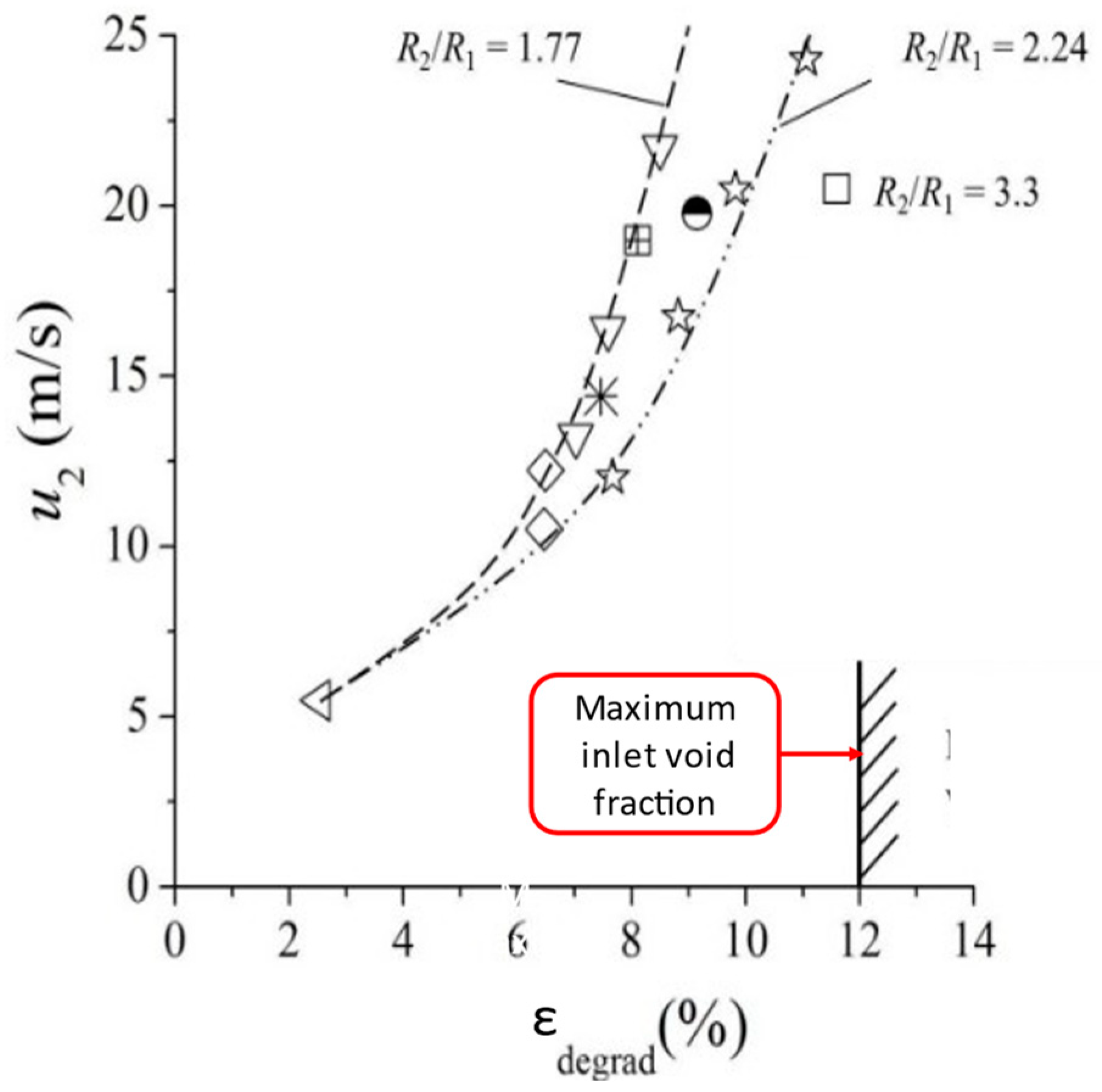
5.3. Surging Criteria Detection

An interesting model to predict the operational conditions that cause two-phase pump surging is proposed by Barrios and Prado [17]. In this approach, surface tension and rotational speed are involved in determining the flow patterns and in predicting the occurrence of stagnant bubbles at the channel intake. These two variables were not present in the models presented in previous sections of the present paper. This model depends on two important variables, namely the stagnant bubble size and the bubble drag coefficient. A bubble size correlation is presented with a new correlation for the drag coefficient as a function of rotational speed and Reynolds number. Not many authors refer to such a work.

6. Conclusions

The present part A brings together the main two-phase flow definitions usually used for pumps and different approaches based on correlation and one-dimensional models that are proposed in the open literature.

Close to the best efficiency point, these models can predict pump performances under two-phase flow conditions accurately when homogeneous conditions are present. For off-design conditions and high inlet void fraction, the only way to predict the performances within an error of ±20% is to adapt interfacial loss and deviation outlet angle models.

For centrifugal pumps, because of strong 3D effects, the one-dimensional approach is limited to a small range of void fractions and is very dependent on bubble sizes that govern interfacial losses. Radial impeller flow channels display significant non-uniformity in void fraction distributions in the transverse as well as in meridional directions. This means that chum-turbulent flow and low-void fraction bubbly flow may co-exist at a given location.

This is the reason why an appropriate 3D CFD approach is necessary to obtain a better local flow understanding (see Part C) in association with the local experimental analysis presented in Part B.

References

1. Gamboa, G.; Prado, M. Experimental Study of Two-Phase Performance of an Electric Submersible Pump Stage. SPE Prod. Oper. 2012, 27, 414–421. [Google Scholar] [CrossRef]
2. Estevam, V.; França, F.A.; Alhanati, F.J.S. Mapping the performance of centrifugal pumps under two-phase conditions. In Proceedings of the 17th Congress of Mechanical Engineering, COBEM 2003, Sao Paulo, Brasil, 10–14 November 2003. [Google Scholar]
3. Barrios, L. Visualization of Multiphase Performance inside an Electrical Submersible Pump. Ph.D. Thesis, The University of Tulsa, Tulsa, OK, USA, 2007. [Google Scholar]
4. Verde, W.M.; Biazussi, J.L.; Sassim, N.A.; Bannwart, A.C. Experimental study of gas-liquid two-phase flow patterns within centrifugal pumps impellers. Exp. Therm. Fluid Sci. 2017, 85, 37–51. [Google Scholar] [CrossRef]
5. Zhu, Z.J.; Zhang, H.Q. A Review of Experiments and Modeling of Gas-Liquid Flow in Electrical Submersible Pumps. Energies 2018, 11, 180. [Google Scholar] [CrossRef]
6. Jiang, Q.; Heng Liu, X.; Zhang, W.; Bois, G.; Si, Q. A Review of Design Considerations of Centrifugal Pump Capability for Handling Inlet Gas-Liquid Two-Phase Flows. Energies 2019, 12, 1078. [Google Scholar] [CrossRef]
7. Baker, O. Design of pipelines for simultaneous oil and gas flow. Oil Gas J. 1954, 26. [Google Scholar]
8. Shaoa, C.; Lia, C.; Zhoua, J. Experimental investigation of flow patterns and external performance of a centrifugal pump that transports gas-liquid two-phase mixtures. Int. J. Heat Fluid Flow 2018, 71, 460–469. [Google Scholar] [CrossRef]
9. Gülich, J.F. Centrifugal Pumps; Springer: Berlin/Heidelberg, Germany, 2010; ISBN 978-3-642-12823-3. [Google Scholar] [CrossRef]
10. Stel, H.; Ofuchi, E.M.; Sabino, R.H.G.; Ancajima, F.C.; Bertoldi, D.; Neto AM, M.; Morales RE, M. Investigation of the Motion of Bubbles in a Centrifugal Pump Impeller. ASME J. Fluids Eng. 2018, 141, 031203. [Google Scholar] [CrossRef]
11. Ofuchi, E.M.; Silva, H.L.V.; Bertoldi, D.; Mancilla, E.; Stel, H.; Morales, R.E.M. Study of the bubble motion in a centrifugal rotor based on visualization in a rotating frame of reference. Chem. Eng. Sci. 2022, 259, 117829. [Google Scholar] [CrossRef]
12. Mikielewicz, J.; Gordon Wilson, D.; Chan, T.; Goldfinch, A. A Method for Correlating the Characteristics of Centrifugal Pumping Two-Phase flow. J. Fluids Eng. Trans. ASME 1978, 100, 395–409. [Google Scholar] [CrossRef]
13. Furuya, O. An Analytical Model for Prediction of Two-Phase (Non condensable) Flow Pump Performance. J. Fluids Eng. Trans. ASME 1985, 107, 139–147. [Google Scholar] [CrossRef]
14. Minemura, K. Prediction of Air-Water Two-Phase Flow Performance of a Centrifugal Pump based on one-dimensional Two- Fluid Model. ASME J. Fluid Eng. 1998, 120, 327–334. [Google Scholar] [CrossRef]
15. Hench, J.E.; Johnston, J.P. Two-Dimensional Diffuser Performance with Subsonic, Two-Phase, Air-Water Flow. ASME J. Basic Eng. 1972, 94, 105–121. [Google Scholar] [CrossRef]
16. Zuber, N.; Hench, J.E. Steady State and Transient Void Fraction of Bubbling Systems and Their Operating Limits. (Part I, Steady State Operation); Technical Report No. 62GL100; General Electric Co.: Boston, MA, USA, 1962; 334p. [Google Scholar]
17. Barrios, L.; Prado, M.G. Experimental Visualization of Two-Phase Flow Inside an Electrical Submersible Pump Stage. ASME J. Energy Resour. Technol. 2011, 133, 042901. [Google Scholar] [CrossRef]
Figure 1. Experimental results of two-phase electric submersible pump (ESP) stage performances at best efficiency (be) point. Non-dimensional head versus liquid flow rate for several inlet void fraction values ε. (Data from Gamboa and Prado [1]).
Ijtpp 08 00016 g001
Figure 2. Example of two-phase mapping (Data from Estevam et al. [2] and Barrios [3] for ESP pumps.
Ijtpp 08 00016 g002
Figure 3. Flow two-phase regime patterns inside the impeller with increasing inlet void fraction (from left to right sides): (a) bubbly; (b) agglomerate bubbly; (c) gas pocket; (d) segregated. (Data from Verde et al. [4]).
Ijtpp 08 00016 g003
Figure 4. Pump head degradation ratio versus inlet void fraction. Each curve and symbol correspond to individual published results at pump design point from different authors that can be found in Jiang et al. [6].
Ijtpp 08 00016 g004
Figure 5. Effects of the impeller outlet rotational speed on the value of εdegrad. Each curve and symbol correspond to individual published results at pump design point from different authors that can be found in Jiang et al. [6].
Ijtpp 08 00016 g005
Figure 6. Two-phase flow patterns inside horizontal pipes (Data from Baker [7]).
Ijtpp 08 00016 g006
Figure 7. Blade to blade plane of a centrifugal impeller with backswept blades.
Ijtpp 08 00016 g007
Figure 8. Meridional plane of a centrifugal impeller.
Ijtpp 08 00016 g008
Figure 9. Blade-to-blade axial flow impeller passage.
Ijtpp 08 00016 g009
Figure 10. Blade-to-blade radial flow impeller passage.
Ijtpp 08 00016 g010
Figure 11. From top to bottom: example of radial evolutions of velocity ratio S V , head loss coefficient and void fraction α inside an impeller channel at best efficiency point for different values of the inlet void fraction ε (Data from Minemura et al. [14]).
Ijtpp 08 00016 g011
Figure 12. Evolutions of several head loss coefficients versus inlet void fraction for two different flow coefficients: top figure: below best efficiency point, bottom figure: best efficiency point. (Data from Minemura et al. [14]).
Ijtpp 08 00016 g012
Disclaimer/Publisher’s Note: The statements, opinions and data contained in all publications are solely those of the individual author(s) and contributor(s) and not of MDPI and/or the editor(s). MDPI and/or the editor(s) disclaim responsibility for any injury to people or property resulting from any ideas, methods, instructions or products referred to in the content.