
Enhancement of Rotor Loading and Suppression of Stator Separation through Reduction of the Blade–Row Gap

1
Aeroengine Research Institute, Beihang University, Beijing 100191, China
2
School of Energy and Power Engineering, Beihang University, Beijing 100191, China
*
Author to whom correspondence should be addressed.
Int. J. Turbomach. Propuls. Power 2023, 8(1), 6; https://doi.org/10.3390/ijtpp8010006
Submission received: 12 October 2022
/
Revised: 11 February 2023
/
Accepted: 22 February 2023
/
Published: 1 March 2023
Abstract
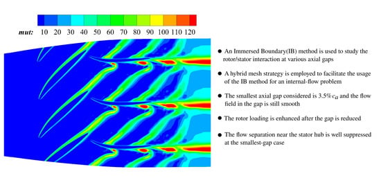
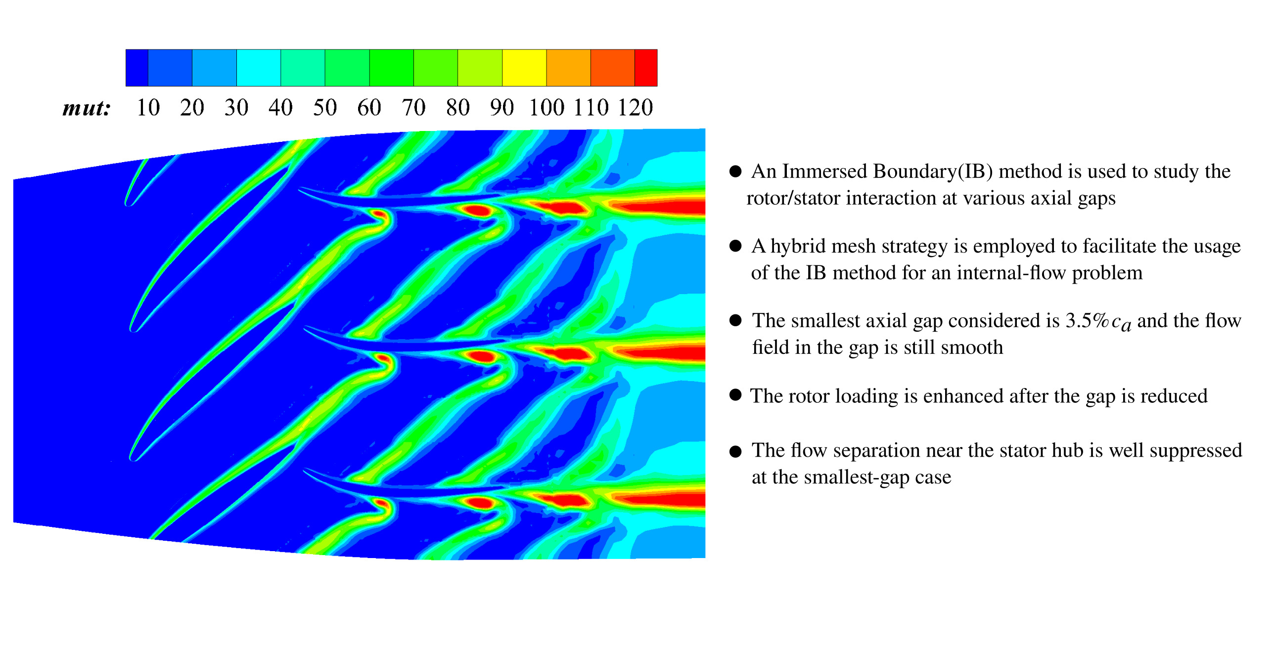
:An immersed boundary (IB) method is applied to study the effect of the blade–row gap in a low-speed single-stage compressor. The advantage of using an IB method is that the rotor/stator interface can be eliminated and, thus, the blade–row interaction can be considered at an extremely small gap. The IB method was modified to internal-flow problems, and the adaptive mesh refinement (AMR) technique, together with a wall model, used to facilitate the simulations for high Reynolds-number flows. The results showed that both the pressure rise and the efficiency were observed to be higher in the smaller-gap cases. Comparisons between the results of two gaps, and , are highlighted and further analysis at a specific flow coefficient showed that the increase of the stage performance was contributed to by the enhancement of rotor loading and the suppression to the flow separation of the stator. Correspondingly, the increases of the total pressure rise on the rotor and the stator outlets were observed to be and , respectively. Although the increase on the rotor outlet is much lower than that on the stator outlet, its significance is that a higher level of static pressure is formed near the hub of the gap, which, thus, reduces the adverse pressure gradient of this region in the stator passage. This improvement suppresses the flow separation near the hub of the stator and, thereby, results in a considerable increase to the pressure rise on the stator outlet as a consequence. The effect of the gap on unsteady pressure fluctuation is also presented.
1. Introduction
The axial blade–row gaps in a multi-stage compressor are significant in the determination of its overall size and weight. Due to the endless pursuit of reducing the size and weight of a machine, it is desirable for the gaps to be as small as possible. However, stronger blade–row interactions exist at smaller gaps, which plays a significant role in the aerodynamic performance, as well as the flow variations, and the corresponding effect is complex and not fully understood.
Normally, for a low-speed compressor, its pressure rise and efficiency increase as the gaps reduce. This phenomenon was confirmed by the experimental studies of Smith [1], Mikolajczal [2]. The theoretical analysis of Smith [3] showed that the evolution of the rotor wake in the stator could help to improve its velocity deficit. A model was proposed by Adamczyk [4] to analyze the recovery process of the total pressure deficit for the rotor wake. The main idea of Smith [3], Adamczyk [4] was that reduction of the gaps could prevent the rotor wake being fully mixed out before it entered the stator passage; thus, decreasing the mixing loss and resulting in enhancement of performance. This mechanism was also reported by Deregel and Tan [5] through a numerical study. On the contrary, for a transonic compressor, reducing the blade–row gap might have a negative impact on aerodynamic performance, as the process of shock–vortex plays a significant role in the generation of loss. A smaller blade–row gap might enhance the interaction of shocks and vortices, and increase the loss in consequence [6,7,8,9]. The present study only focuses on the gap effect in a low-speed condition.
In the works of Smith [3], Adamczyk [4], Deregel and Tan [5], the variation of the rotor loading was not considered and the contribution of the rotor to the performance enhancement was unknown. Actually, it is also challenging to measure the flow characteristics of a rotor or in a blade–row gap, which means it receives less attention. Later, Du et al. [10,11] conducted a number of numerical simulations to the blade–row interactions at different gaps and found that the rotor would work at a higher-loading state as the gap reduced. A vortex lift mechanism was also proposed by Du et al. [10,11] to explain this phenomenon because unsteady vortex shedding at the trailing edge of the rotor was observed when the rotor blade swept over a stator vane. The vortices were enhanced by the reduction of the gap due to the stronger blade–row interaction, thus increasing the fluctuation, as well as the average, of the rotor loading. The unsteady process of vortex shedding was confirmed by Xu et al. [12] through PIV measurements in a tiny pump, and higher rotor lift was also obtained at the smaller gaps in their numerical simulations. The studies of Du et al. [10,11] through 2D simulations suggested that the rotor loading could be changed through reducing the gap. A significant issue is the dependence of rotor loading on the stage gap in 3D flow condition, which is of interest to the present study.
When multiple blade rows are considered in the simulations, mesh interfaces are constructed between the blocks of different blade rows and additional treatments to the interfaces are necessary. Rai [13], Jorgenson and Chima [14] used patched and overlaid grids for rotor/stator configurations to simulate the unsteady effect of blade–row interaction. A layer of shearing cells between the grids of the rotor and the stator were adopted by Giles [15] in the unsteady simulations for a transonic turbine. Although the above techniques for rotor/stator interfaces are widely used in practice, a defect is that when two blade rows are very close to each other, e.g., the gap is less than , it is difficult to ensure the mesh quality at the gap of the blade rows, and sometimes it is even impossible to generate an available mesh for the case with an extremely small row gap. Due to this limitation, the minimum axial gap in most numerical studies considering the effect of blade–row gap, e.g., see Hsu and Wo [16], Przytarski and Wheeler [17], appeared to be about 10∼30% , and investigations at smaller gaps have not yet been reported. In addition, the flow information exchange at the block interfaces also results in additional errors when the mesh between the two rows is highly distorted at a small gap. As a consequence, the numerical reliability is highly questionable in this situation.
The difficulties mentioned above can be overcome by using immersed boundary (IB) methods, which can efficiently deal with moving boundary problems and complex geometries [18,19,20]. Zhong and Sun [21] reported the application of an IB method to the flutter problem in turbomachinery, and Du et al. [10,11] investigated the effect of rotor/stator interaction at small stage gaps and also considered the aerodynamic benefit of pitching the stator through an IB method. Chen et al. [22] used an IB method to compute the unsteady blade loading for a compressor at a small gap and its profile showed good agreement with the experimental data. With a high-order scheme employed, IB methods can also be used to study the acoustic resonance induced by blade vibration [23]. These numerical studies exhibited the ability of IB methods to simulate the unsteady problems in turbomachinery with multiple blades included, which, however, were only restricted to 2D configurations and, thus, could be performed on Cartesian grids. For 3D and turbulent flow conditions with moving boundaries, due to the enormous grids needed by the Cartesian grids, there are less related investigations. To consider the turbulence effect when an IB method is employed, adaptive mesh refinement (AMR) [24,25,26,27,28] and wall functions [29,30,31,32,33,34], are two common routes to accelerate the simulations, and they have mainly been applied to the external-flow conditions. For internal-flow problems, which are of interest to the present study, the flow channels can be larger than the internal bodies. Directly resolving the flow channels by using a Cartesian grid results in an extra large number of cells, which might be unaffordable. How to achieve efficient simulations for 3D high Reynolds-number internal flows by using IB methods still lacks deep investigation. This paper adopts a hybrid mesh strategy with a single-block body-fitted mesh to the flow channel and an IB method to model the internal bodies, and with some modifications, the IB method can be extended to a general curvilinear grid. With these techniques, the effect of reducing gap can be studied easily by using an IB method with affordable computational costs.
This paper presents a numerical study, conducted in our laboratory, on the effect of stage gap in a low-speed single-stage compressor, termed TA36 in the published works [35,36,37,38,39]. The AMR technique was adopted to the IB method to dynamically enhance the local mesh resolution for both the rotor and the stator. A wall function was used to further improve the efficiency of simulations for high Reynolds-number internal flows. The enhancement of performance contributed by the rotor and the stator individually, as well as the corresponding flow variations, is of great interest. The paper is organized as follows: Section 2 introduces the numerical methods employed, including the governing equations, the grid formation and the IB method adapted to the internal-flow problems. Comparisons to the experimental data are given as a validation and the numerical convergence is also examined. Then, simulations are conducted at two different gaps and the corresponding results presented and discussed in Section 3, including the overall performance enhancement and its spanwise distribution, the flow mechanism and the unsteady characteristics. Finally, a brief conclusion is drawn in Section 4.
2. Numerical Methods
2.1. Governing Equations
The flows are governed by the three-dimensional compressible Navier–Stokes equations, and their conservative forms are written as follows:
where is the flow velocity vector. is the total energy per unit mass and represents the total enthalpy per unit mass. is the friction stress tensor and its component can be computed as:
is obtained following the Sutherland’s law. is the heat flux, written as follows:
The ideal-gas law is:
The turbulent behaviors are modeled by solving the unsteady Reynolds-Averaged Navier–Stokes (URANS) equations with the one-equation Spalart–Allmaras (SA) model [40], and the governing equation for the turbulence field variable is written as follows:
The turbulence eddy viscosity, , is computed from:
The convective flux on cell faces is evaluated by the standard Roe scheme [41], and a low-speed modification [42] is implemented for low Mach number flow conditions. To achieve second-order spatial accuracy, the MUSCL interpolation [43] is employed within cells to reconstruct the variable distribution. A second-order central difference scheme and a third-order Runge–Kutta scheme are applied to compute the viscous flux and the temporal derivatives, respectively.
2.2. Grid Strategy
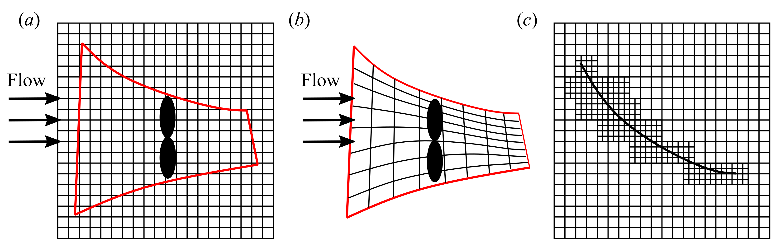
Traditional IB methods always model a wall boundary on a Cartesian mesh and the mesh refinement to a specific region also increases the cell density in the far field. The corresponding computational cost is unaffordable when the flow is 3D and turbulent, which also constrains further application of IB methods. For the turbomachinery applications, because the flow channels are usually not conformal to a cuboid, Cartesian grids, which are larger than the channels, are necessary if the IB method is used to model both the flow channel and the blades, as shown by the example in Figure 1a. In the case of Figure 1a, to meet the requirement of resolution, both the channel walls and the blades need to be resolved by additional grid refinement, which can result in enormous extra cells in the simulations using a Cartesian grid, especially under high Reynolds-number conditions. However, the flow channel is always stationary and makes no contribution to the unsteadiness we are interested in, and there is no need to model the channel by the IB method.
Therefore, a hybrid mesh strategy, in which a body-fitted mesh to fit the flow channel and then an IB method was used only to model the blades in the present work. Firstly, a single-block structured curvilinear mesh was used to fit the channel as background mesh, as shown by Figure 1b. With the body-fitted mesh to the channel, the boundary conditions of the channel walls were imposed through the same manner with the traditional body-fitted methods, which can help to avoid using additional cells to resolve the flow channel by the IB method. Then, to locally enhance the mesh resolution near the blades modeled by the IB method, the adaptive mesh refinement (AMR) technique was employed to increase the grid density near the blades without producing extra cells in the far field, as shown in Figure 1c. AMR has been proved to be an effective method to locally enhance the mesh resolution for high-gradient flow structures [44,45] or wall boundaries [26,27,46]. As a consequence, the cell number can be reduced remarkably for the 3D and turbulent cases compared with the traditional IB approaches. Note that in the present mesh strategy, the IB method was performed on a curvilinear grid instead of a Cartesian grid, and the following section introduces the imposition of boundary conditions for the blade.
2.3. Internal Blade Treatment
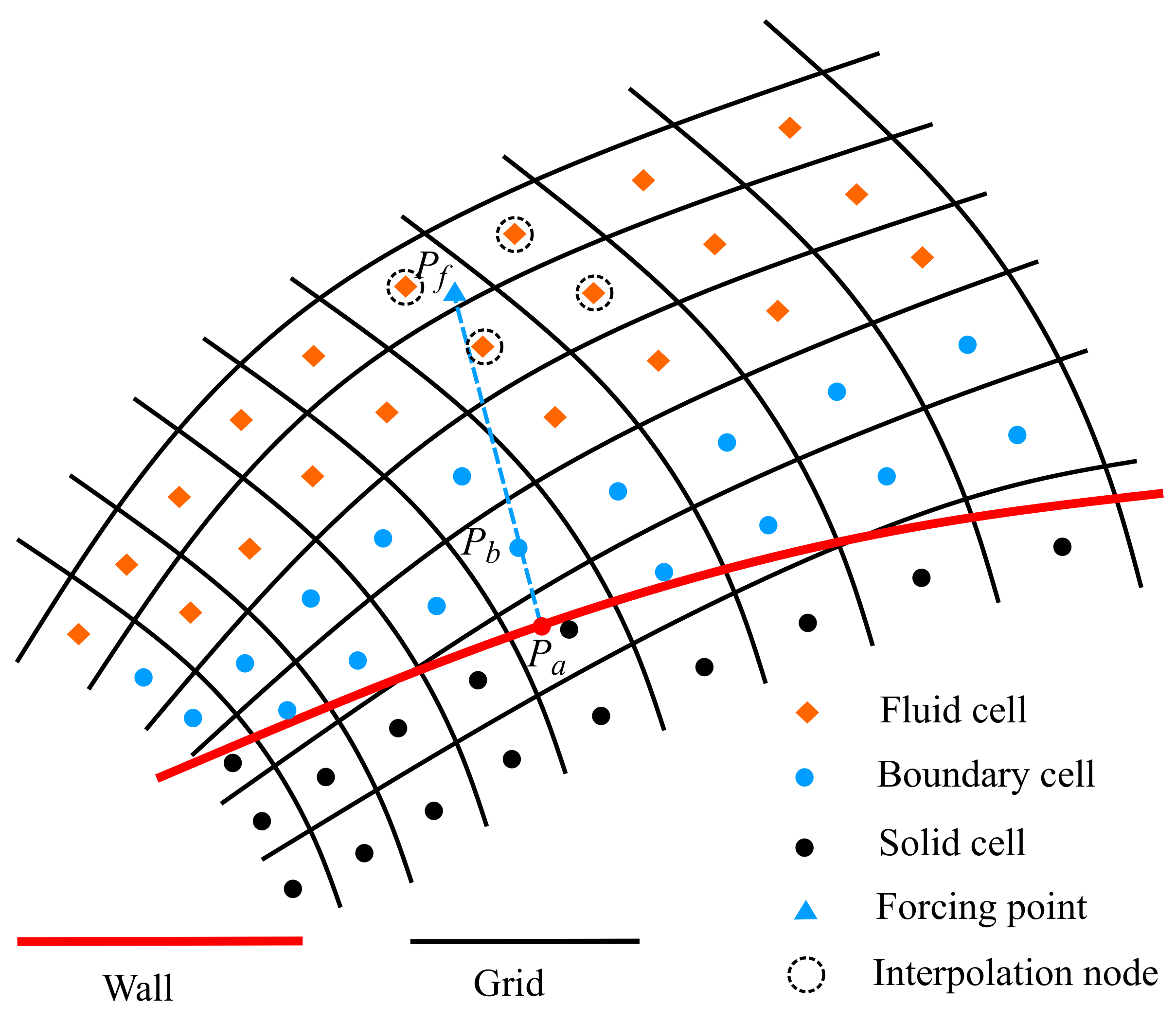
To model the internal blades, a sharp interface IB method, which was first proposed by Gilmanov et al. [47], Gilmanov and Sotiropoulos [48] for the Cartesian grid, was used here. All the grid cells are firstly categorized into two types: fluid cell and solid cell, which are at the exterior and the interior of the internal walls, respectively, as shown in Figure 2. The flow quantities of the solid cells are insignificant. Further, the two layers of fluid cells which are adjacent to the solid cells are identified as boundary cells, so that the solid cells are not involved in the calculation of spatial derivatives. The flows at the rest of fluid cells are determined by solving the governing equations.
To impose the boundary condition for each boundary cell, e.g., in Figure 2, a forcing point surrounded by fluid cells is first obtained, termed . is normal to the wall, with being the projection point on the wall. With the flow quantities at and known and assumed distributions for the flow quantities within the boundary layer adopted by the IB method, the quantities at can also be obtained. The distance between and is termed forcing distance in this paper. For the traditional sharp interface IB methods on a Cartesian grid, the forcing distances are usually fixed for all boundary cells, which is not appropriate when the grid is curvilinear and contains large aspect ratio cells. As shown by Figure 3, where the walls with different orientations are surrounded by the large aspect ratio cells, for the boundary cells and , which are close to the walls and , respectively, the same forcing distance can locate their forcing points at and , respectively. is close to an adjacent cell of and using the quantities at to impose the boundary condition at is reasonable. In contrast, there are several fluid cells between and , the flows of which are obtained from solving the equations instead of assumed profiles. Therefore, is invalid for and a more close forcing point to is desired. To ensure the close cell to is adjacent to the boundary cells, the forcing distance is adaptively determined for different boundary cells, with their aspect ratio considered. Therefore, there are only a few cells between and , which can ensure the hypothesis for the quantity distributions between the two points is valid.
The inverse distance–weight (IDW) interpolation is applied to compute the flow quantities at the forcing point from its adjacent flow cells. For the ith interpolation stencil cell, the corresponding weighted coefficient can be written as:
where is the distance from the forcing point to the ith stencil cell. k is the power coefficient and set as 2. To further obtain the tangential velocity at , an explicit turbulence wall function [49] is employed, given as Equation (8):
A linear distribution is assumed for the normal component of the flow velocity. The pressure gradient along the normal direction of the wall is assumed to be zero; therefore, the pressure at equals that at . The temperature is determined by the Crocco–Busemann relation:
where denotes the tangential velocity. A linear relation is used to compute at the boundary cells:
where is the distance from a boundary cell to the wall.
2.4. Comparison to the Experimental Data and Convergence
The model of an in-house compressor, TA36, was considered in the present numerical study. This testing rig was designed for the study of flow instability in the compressor and thorough experimental results at the designed gap have been provided [35,36,37,38,39]. Its rotor and stator consist of 20 and 27 blades, respectively, with a gap of . The designed working speed is 2930 rpm. The outer diameter is 600 mm and the hub-to-tip ratio at the domain outlet is . More parameters about the testing rig can be found in the published works.
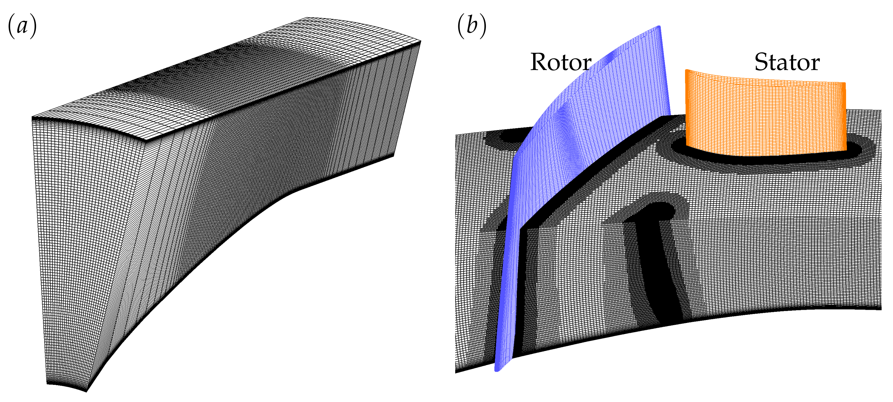
In this study, a sector domain was considered, where both the rotor and the stator were modeled by using the IB method. The inlet and the outlet of the domain were placed at upstream the rotor’s leading edge and downstream the stator’s trailing edge, respectively. Only a single passage was considered for each blade row, and, therefore, the blade number ratio of the rotor and the stator was reduced to 1:1. The stator blade was enlarged along the chordwise direction in simulations so that its solidity could remain the same with the real machine. A single-block structured mesh was used to fit the sector domain as the background mesh, as shown in Figure 4a, which consisted of cells. Then, AMR considering the blade locations was carried out on the background mesh, producing additional levels to resolve the blades, as shown in Figure 4b. The mesh refinement was dynamically adjusted to keep the mesh resolution around the rotor blade. The total pressure and the total temperature were fixed at the domain inlet and a back pressure was prescribed at the domain outlet. The no-slipping boundary condition was employed for the shroud, the hub and the blades, and the periodic boundary condition was adopted along the circumferential direction.
To examine the grid convergence, simulations were conducted at the designed stage gap by using grids with different numbers of refinement levels, from 3 to 6. In brief, the grids were termed in the form of IB-X, where X denotes the number of the refinement level. The refinement of AMR was performed through a distance criterion. For each cell of a coarse grid level, their closest distance to the blades was calculated and if they were lower than the critical distance set for this level, the corresponding cells would be refined and produced additional cells with higher resolution. The corresponding critical distances for each grid level are provided in Table 1. Consequently, the corresponding total cell numbers of each grid are given in Table 2, which suggests that the total cell number would almost double when one more refinement level was added. For each simulation, the back pressure was increased in a stepwise form with a fixed interval. The flow coefficient is denoted by and its definition is given by Equation (11):
where and is the plane-averaged axial velocity at the domain inlet and the tangential velocity at the rotor mid-span, respectively. All static pressures presented in this paper are normalized through Equation (12):
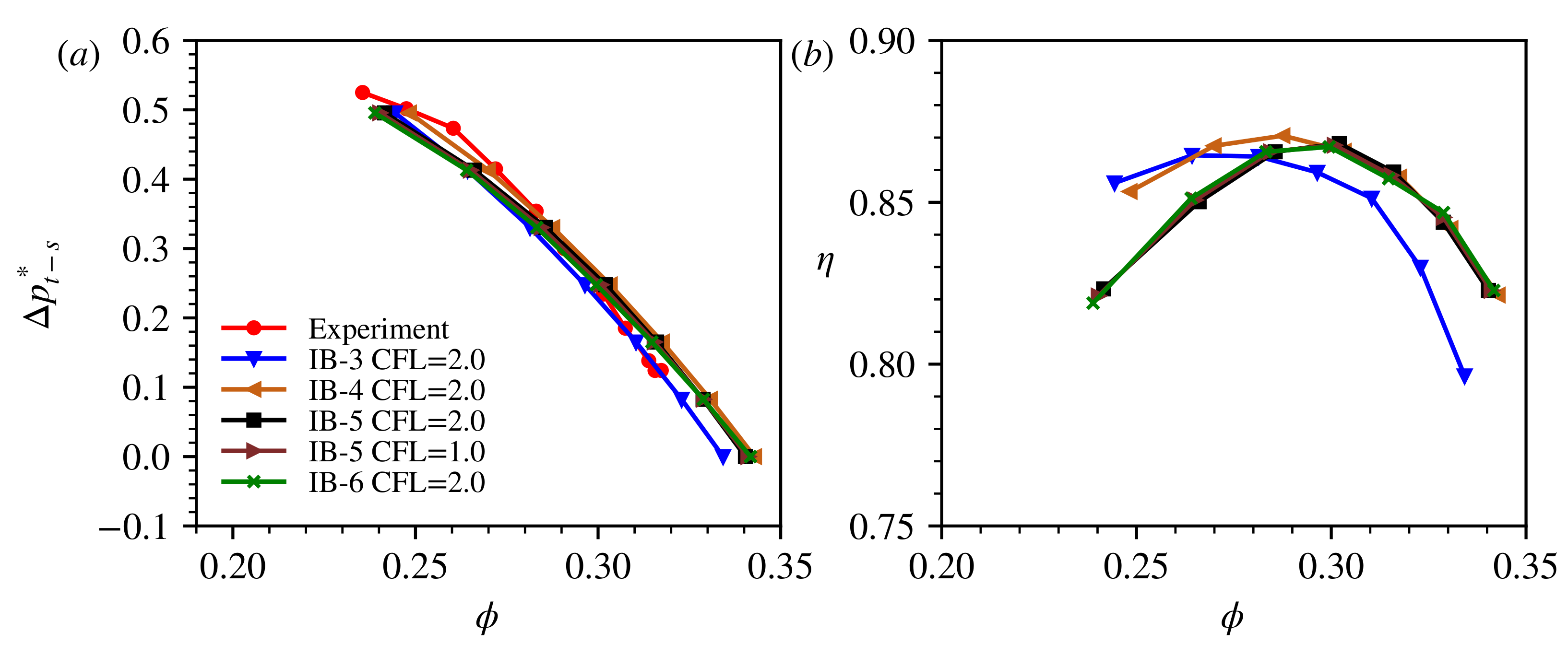
Figure 5 shows the aerodynamic performances obtained by using different grids, including the coefficients of static-to-total pressure rise and the efficiencies. The experimental data of pressure rise is also included in Figure 5a for comparison. As shown in Figure 5a, the characteristic lines obtained by different grids were close to each other, and all of them showed good agreement with the experimental data, indicating good convergences. However, comparisons in Figure 5b revealed obvious discrepancies for the adiabatic efficiencies when there were less numbers of refinement level. To achieve convergence for the efficiency at each flow coefficient, at least 5 grid levels were necessary, and only slight differences could be identified between the efficiencies obtained by the IB-5 and the IB-6 grids. Therefore, the IB-5 grid was used in the following study. Since it was hard to accurately measure the adiabatic efficiencies in experiments of the low-speed compressor, the corresponding experimental results are unavailable. The number was set as 2.0 for all grids, yielding a non-dimensional time step of for the IB-5 grid, with the time for reference being . Therefore, about 13590 steps were needed for the rotor to pass a blade passage. To further examine the independence of results on the time step, a simulation for was also performed for the IB-5 grid. The corresponding results are also included in Figure 5, which only exhibits very slight differences with the results of and, thereby, indicated that using for the IB-5 grid could ensure numerical convergence. The total cell number of the IB-5 grid was almost 10 million, while the traditional body-fitted method might only need about half of them when dealing with the same problem. It is known that more grid cells are necessary for the IB methods than the body-fitted method for high Reynolds-number flows. However, it was better to use the IB method to deal with the rotor/stator interaction at such a small axial gap as that being considered in the present work, since it is very challenging to generate a high-quality mesh with a smooth rotor/stator interface for the body-fitted strategy under this situation. From this perspective, we believe using more grids to overcome this difficulty was worthwhile. For the simulations using the IB-5 grid, time marching for 100 thousands steps costs about 5760 cpu hours. Specifically, the dynamic adjustment due to the rotor’s movement was performed every 55 steps, and the corresponding time cost was about of the total.
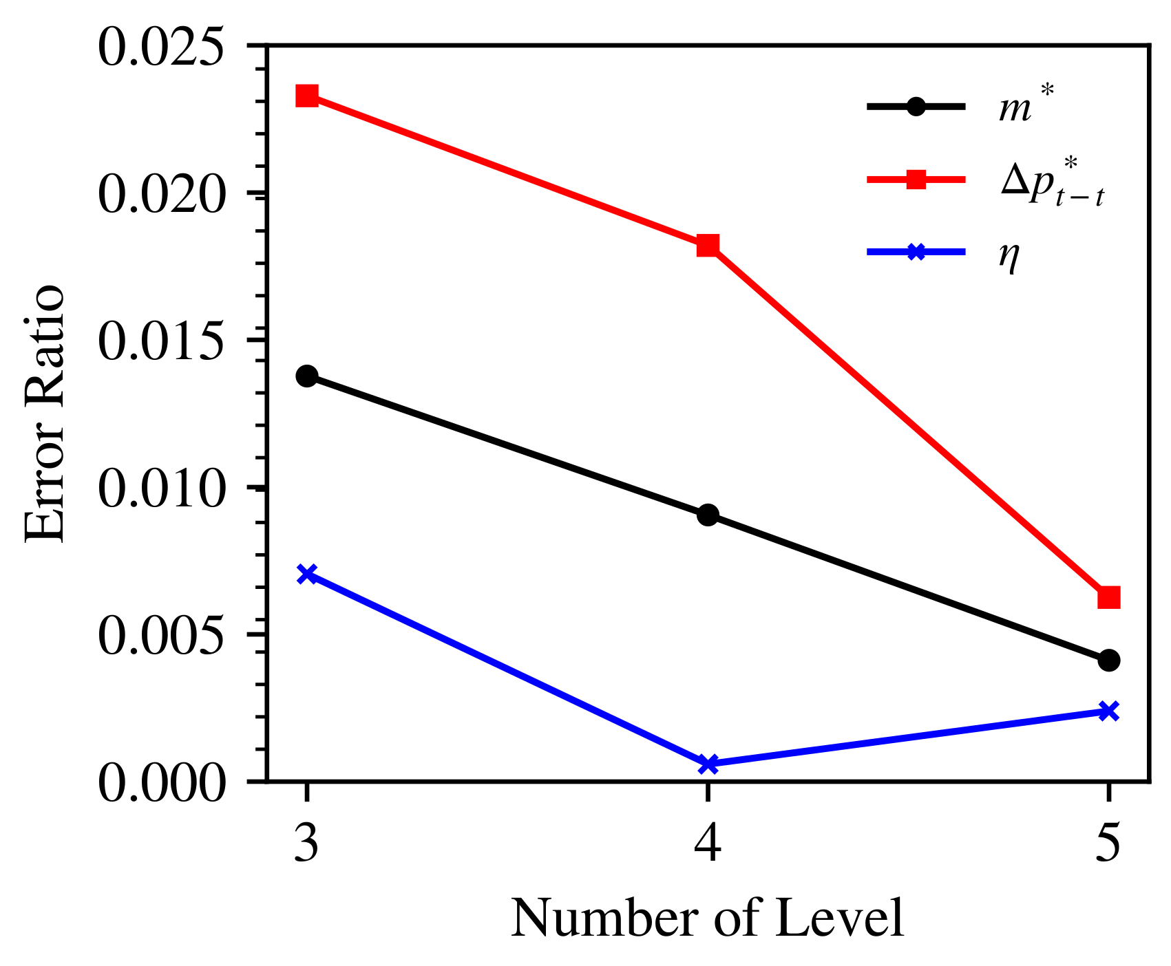
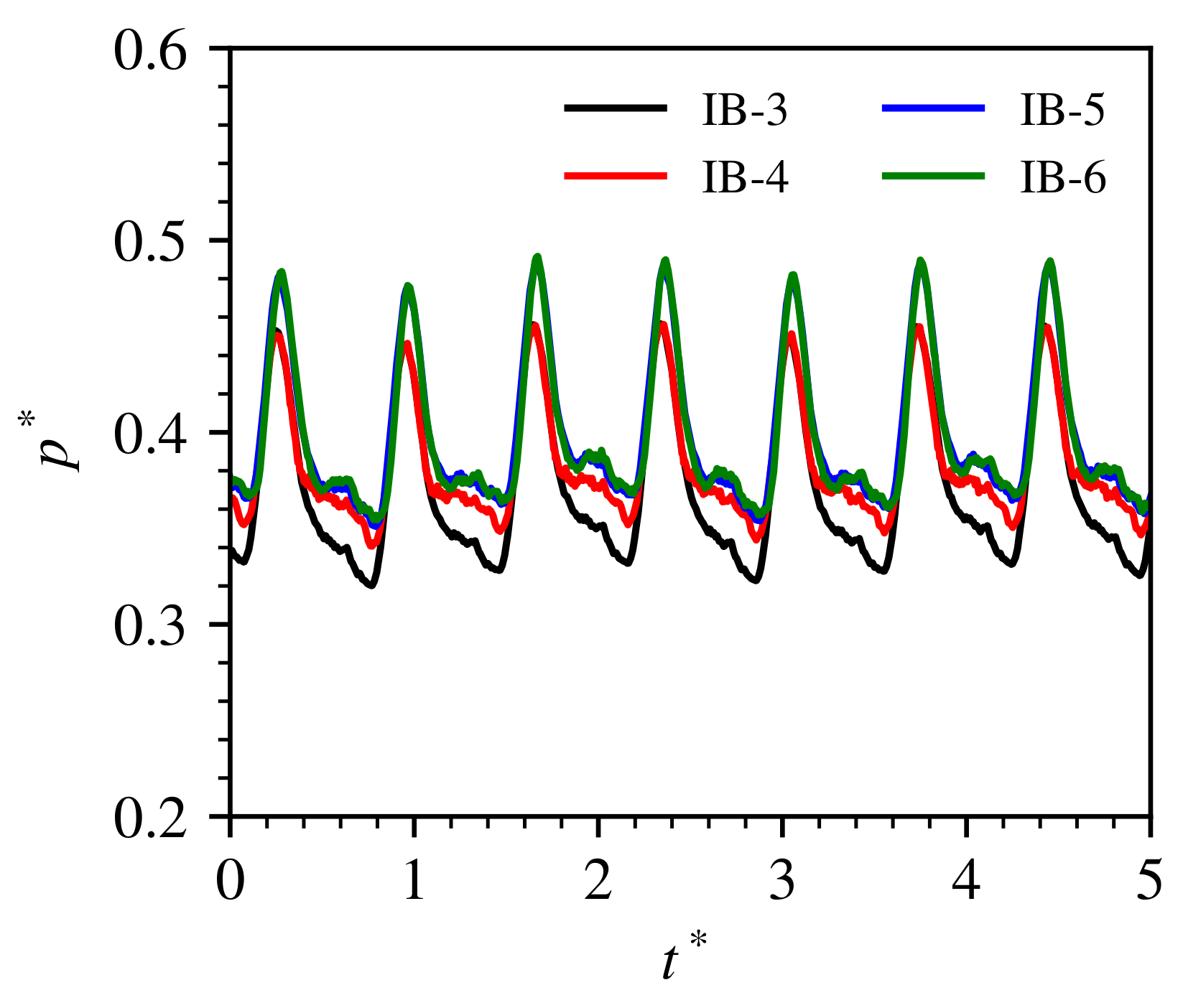
To examine the mass conservation from the inlet to the outlet of the domain, the flow coefficients of the two planes, as well as their differences, obtained by the IB-5 grid, are given in Table 3. The operation conditions were those shown in Figure 5. It can be seen that the largest difference for the mass flow was , which was observed at the near-stall condition, and, in other cases, the differences were more slight. It is, therefore, believed that mass conservation could be ensured when using the present IB method to study the flow of blade–row interaction. The following discussion mainly focuses on the effect of stage gap at the working conditions around . Therefore, to further quantify the convergence under this case, with the corresponding performances obtained by the IB-6 grid treated as reference data, the error ratios, as functions of the number of refinement, are presented in Figure 6, for the flow coefficient, the total-to-total pressure rise and the adiabatic efficiency. It can be seen that both the errors of the flow coefficient and the pressure rise appeared to decrease as the number of level increased, and they were observed to be about for the IB-5 grid. Although the error of the efficiency was observed to grow slightly when the number of level was increased from 4 to 5, the corresponding difference for the IB-5 grid was pretty low, i.e. about . Therefore, using the IB-5 grid could help to balance accuracy and computational cost. Since the unsteady characteristics were of great interest, convergence of the pressure fluctuation at the target flow condition was also illustrated. Figure 7 shows the predicted unsteady pressure profiles of a location on the stator surface, which was near the leading edge of the 90% span section, when different grids were used, and their root-mean-square(R.M.S) values are provided in Table 4. As can be identified from Figure 7, the time profile of the IB-5 grid was consistent with that of the IB-6 grid, and the difference ratio of their R.M.S values was about . Therefore, it is believed that the IB-5 grid could also provide convergent results for the unsteady characteristics.
The distribution of on the rotor blade for the 5-level mesh is plotted in Figure 8. Note that for each segment of the surface, the values were taken from their forcing point. The maximum of appeared to be lower than 100 on both the pressure and the suction surfaces of the blade. Note that the corresponding numerical results in the works of Tamaki et al. [31], Berger and Aftosmis [32], Cai et al. [33], Constant et al. [34] with the same range also agreed well with the data for comparison, which also reinforced our confidence in the present 5-level mesh.
3. Results and Discussions
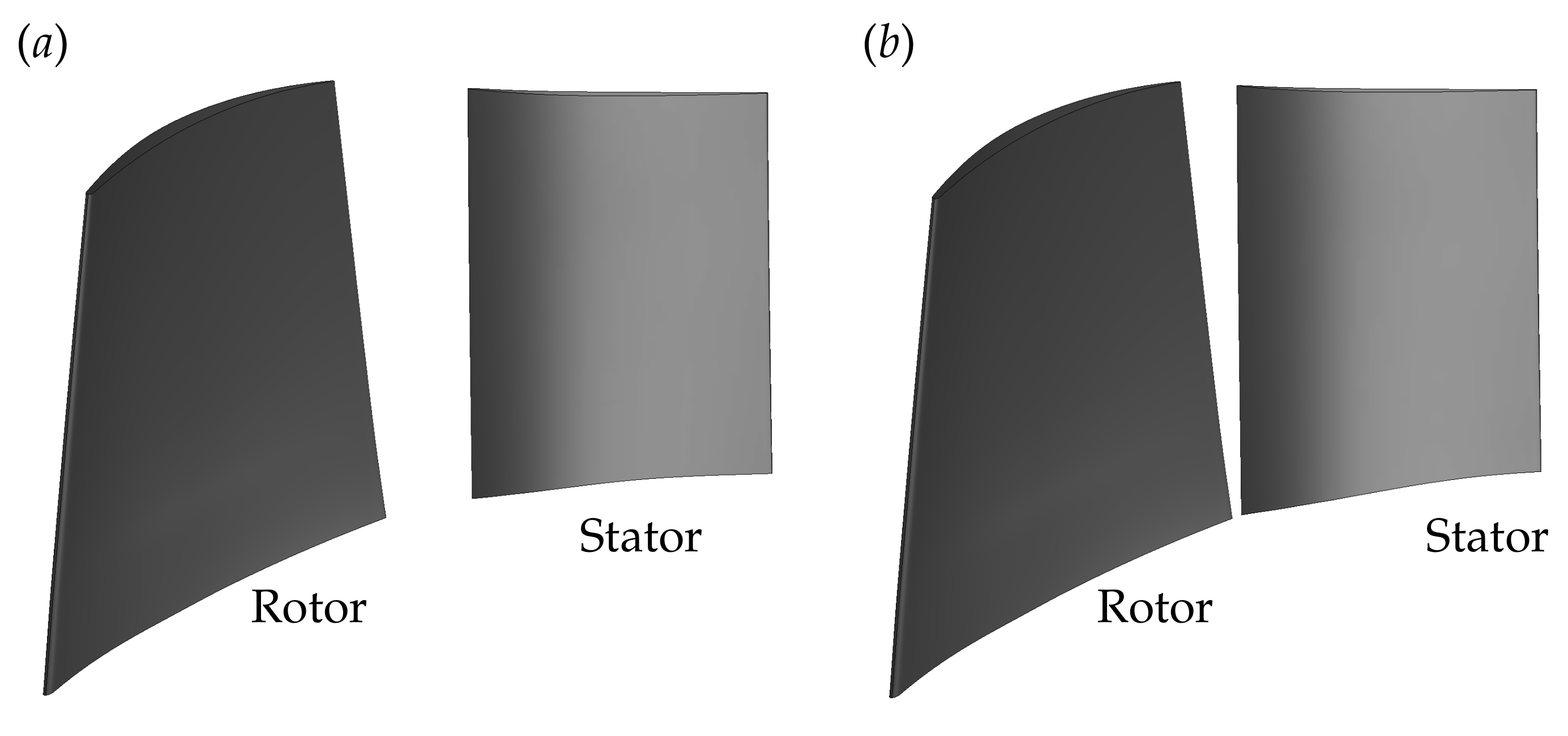
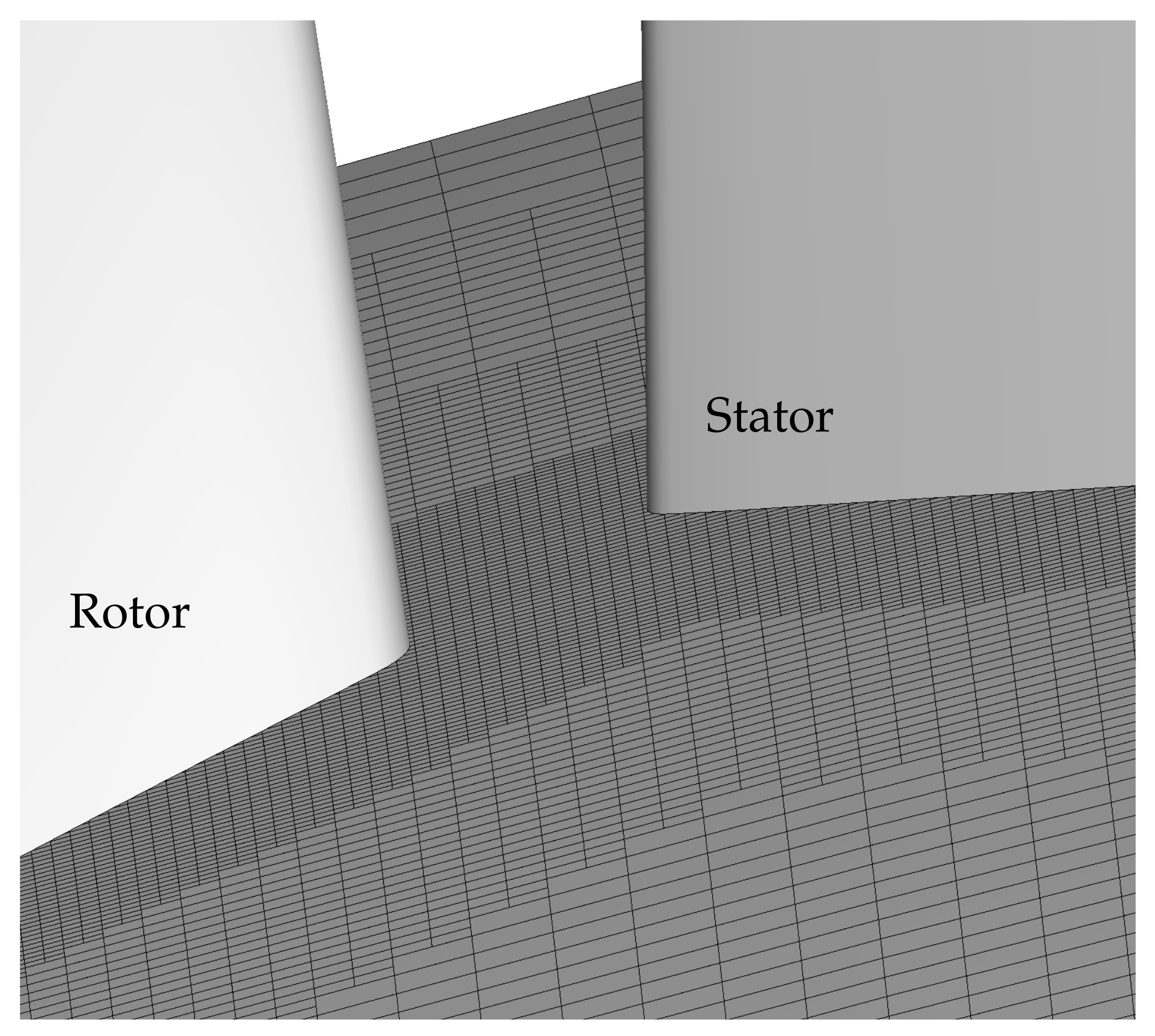
To investigate the effect of the stage gap, the axial distance between the rotor and the stator was reduced to of the designed value, and its effect on the performance and the variation of flow characteristics studied numerically. For the back pressure producing the designed mass flow rate at the designed gap, simulations at the other three moderate gaps were also be performed at the same back pressure in order to examine whether the variation of aerodynamic performance was consistent if the row gap continuously changed. The relative positions of the rotor and stator at the designed gap and its 10% are shown in Figure 9a,b, respectively. Note that the axial distance from the rotor’s trailing edge and the stator’s leading edge on the hub surface was measured as the gap distance in this paper, and the designed value denoted by , i.e., . Reduction to the axial gap was achieved by adjusting the axial location of the stator with the rotor fixed. Specifically, the 5-level mesh on the hub surface for the smaller gap, i.e., , is presented in Figure 10. Generation of a high-quality mesh at such a small gap is challenging to the traditional body-fitted approach, while it can be easily modeled by the IB method. As can be found from Figure 10, there were still about 12 cells in the streamwise direction from the rotor’s trailing edge and the stator’s leading edge on the hub surface. The spatial scheme used in the present study required the first two closest layers of cells near the blade in the fluid domain to be marked as boundary cells, and their forcing points, thus, were always located near the third closest layer of cell near the blade. Therefore, even for the smallest-gap case, shown in Figure 10, the impositions of the boundary condition for rotor and the stator would not influence each other. Moreover, for the designed cases with 10% gaps, the corresponding axial distances from the rotor’s trailing edge and the stator’s leading edge at the tip region were and , respectively.
3.1. Overall Performance at Different Gaps
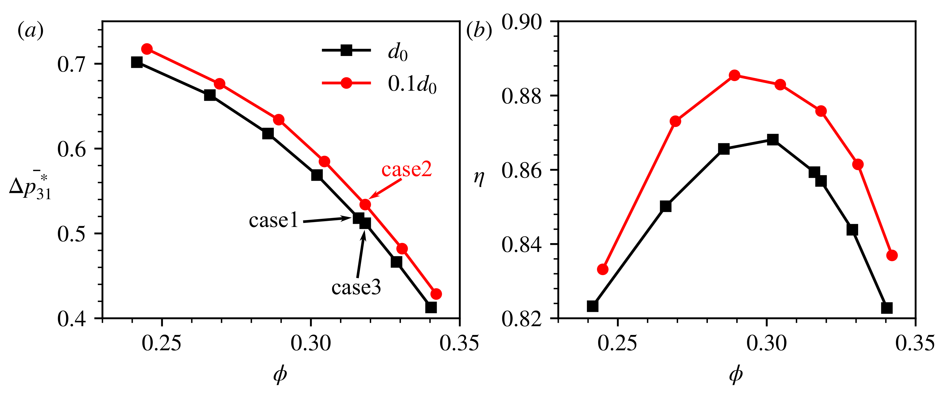
Figure 11a,b show the comparisons of the total pressure rise and the adiabatic efficiency at two gaps, and , respectively, It can be seen, at each back pressure considered, the mass flow rate, the total pressure rise and the efficiency were all observed to be higher at the smaller gap, indicating that performance enhancement could be obtained through reduction of the stage gap. Cases 1–3, marked in Figure 11a, were near the designed working point of the compressor. Cases 1 and 2 had the same back pressure but different gaps, the flow coefficients of which were 0.316 and 0.318, respectively. For cases 1 and 2, reducing the gap from to resulted in increases of , to the flow coefficient and the total pressure rise of the stage, respectively. Besides this, the stage efficiency also increased by . To further demonstrate the effect of row gap under the same back pressure, cases 1 and 2 simulations were also conducted at the other three moderate gaps between and at the same back pressure. Figure 12 shows the variation of the aerodynamic performance as a function of the blade–row gap. As the row gap continuously reduced, higher mass flow rate, total pressure rise and efficiency could be observed, suggesting the dependence of the aerodynamic performance on the row gap was consistent at the designed working point.
For a subsonic compressor, the mixing loss of rotor wake can be reduced when the gap becomes smaller, which was used to explain the generation of performance benefit by Smith [3], Adamczyk [4]. Du et al. [10,11] reported a vortex lift mechanism due to the blade–row interaction and the rotor loading was observed to be higher at a smaller stage gap. Therefore, both the flow variations of the rotor and the stator make some contributions to the performance enhancement of the compressor stage after the gap is reduced. Separating the contributions from the rotor and the stator was the main purpose of this work, which might be challenging in experiments because measurements at a narrow gap are normally not allowed.
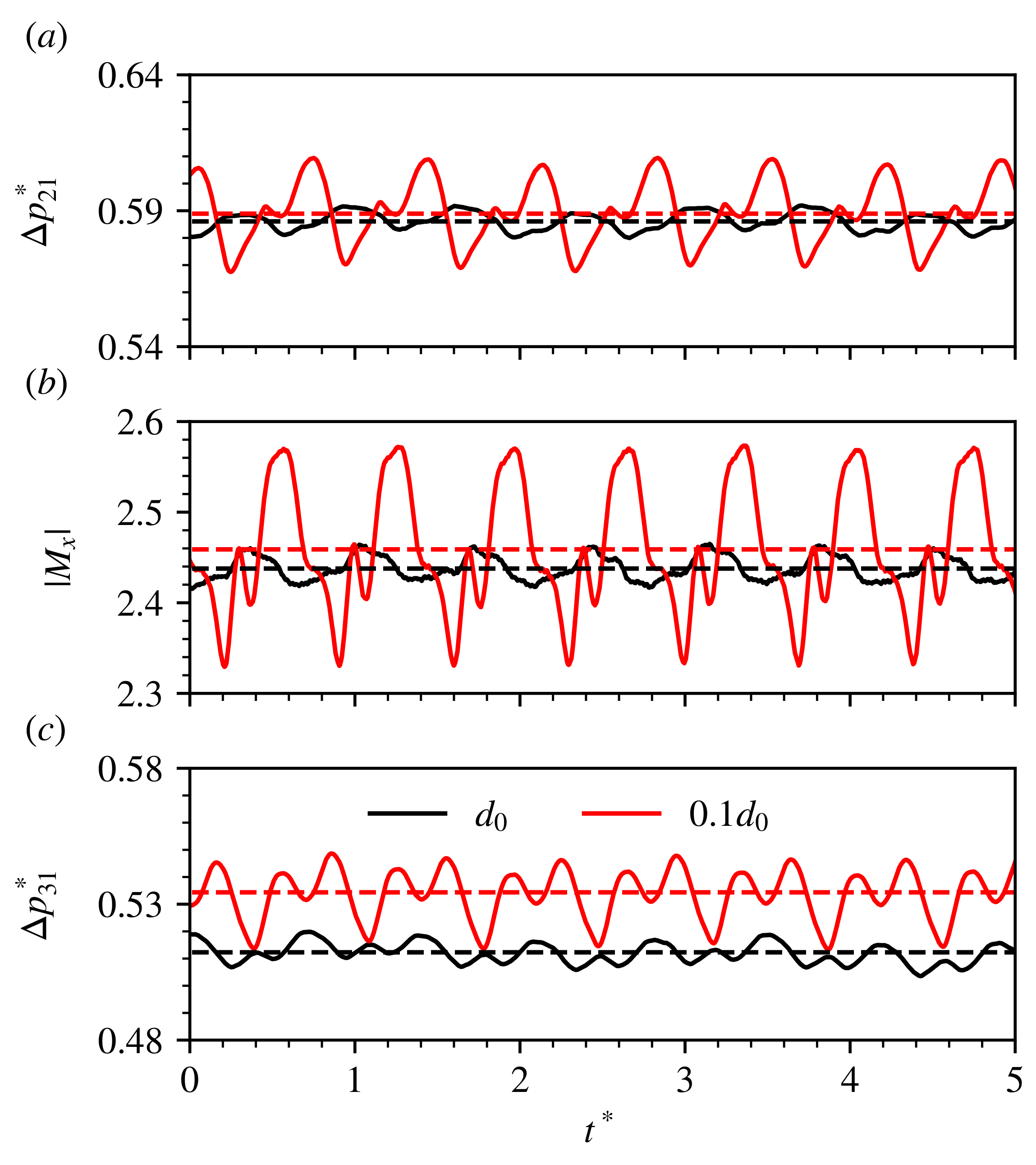
In the following, comparisons are made for the results of cases 2 and 3, the flow coefficients of which were both 0.318. To quantify the contributions of the two blade rows to the performance enhancement individually, Figure 13 shows the time profiles of the total pressure rise on the rotor and the stator outlets, as well as the axial torque of the rotor blade for cases 2 and 3, where their time-averaged values are also plotted through the horizontal dashed lines. It is remarkable that when the gap reduced, their averaged values also appeared to be higher, and increases of and were observed for the averaged total pressure rises on the rotor and the stator outlets, respectively, as shown in Figure 13a,c. Correspondingly, the averaged axial torque on the rotor blade, shown in Figure 13b, was also found to increase by , confirming that the rotor worked at a higher-loading state when the gap reduced. It is noticeable that the benefit from the stator was more outstanding than that from the rotor. The following discussion reveals that, besides the contribution of wake recovery in the stator, the flow separation near the stator hub is well suppressed through the reduction of the stage gap, which results in a great influence on the performance of the stator. The higher pressure in the stage gap due to the increase of rotor loading plays a significant role in the suppression of the flow separation.
Note that the outlets of the rotor and the stator were located at and downstream of their trailing edges, respectively. The rotor outlet was also treated as the stator inlet. Since the variation of gap was achieved by adjusting the axial location of the stator, when the gap changed, the distance from the stator inlet to the stator was slightly different, and this effect was slight as the analysis mainly focused on the quantities of the outlets of the rotor and the stator.
3.2. Spanwise Distributions of the Performance Enhancement
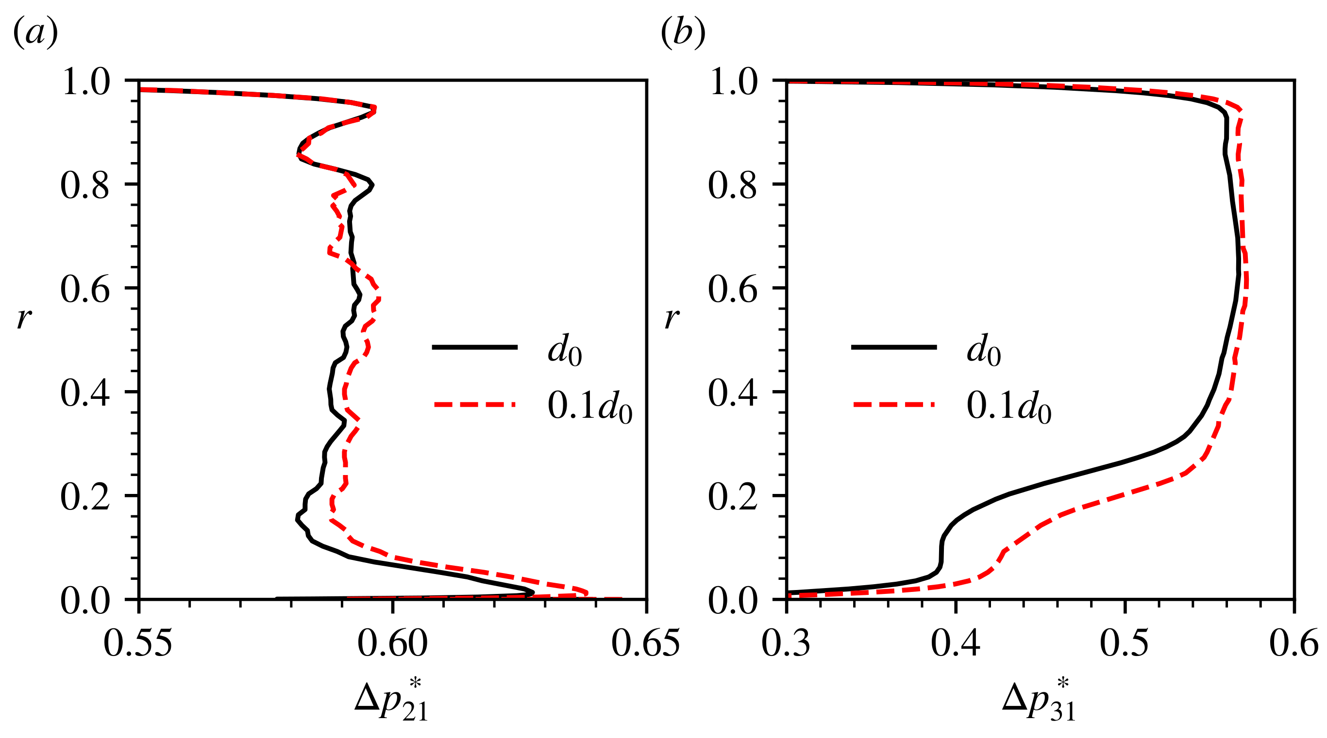
The ratio of performance enhancement for the rotor between cases 2 and 3 appeared to be much lower than that reported by Du et al. [10,11] through 2D simulations. Since the stage gap was non-uniform along the span, as shown in Figure 9, the benefit of reducing the gap might also differ along the span location. To demonstrate this dependence, Figure 14a,b show the spanwise distributions of the averaged total pressure rise on the rotor and the stator outlets, respectively, which were obtained by firstly averaging the transient data along the pitch at each moment and then in a blade-passing cycle. Note that all the spanwise distributions in the following were obtained in this manner without additional mention. To further quantify the differences of performance along the span, Figure 15a also shows the incremental ratios of the total pressure rise on the two planes as the gap reduced. It can be seen from Figure 14 that the variations of performance were obvious in the low-span regions, i.e., , for both the rotor and the stator after the gap reduced. The contributions from the rotor and stator, as well as the corresponding flow variations, were of particular interest and the following discussion focuses on this aspect.
On the rotor outlet, reducing the gap to resulted in increases of for the total pressure rise in the range of , as shown in Figure 14a and Figure 15. In contrast, the benefit in the rest of the span locations was negligible and even negative. Such a variation on the rotor outlet was well related to the nonuniform gap size along the span. Although the gap reduced to an extremely small value at the hub, as shown in Figure 9, the tip region still worked with a considerable gap, i.e., , and, thereby, the rotor performance in the tip region did not exhibit much difference. This clarified that when the gap became small, the spanwise distribution of the gap could be determined well by the 3D blade geometries of the adjacent blade rows. The increase of the total pressure rise in Figure 14a after the gap reduced also suggested that the rotor loading could be enhanced through reducing the gap. Chung and Wo [50] conducted a study to split the potential and the vortical effects at different blade–row gaps and found that the potential effect was important, especially after the gap was less than blade chord. Therefore, in the present case, after the gap reduced to , the potential effect from the stator might play a significant role in the pressure distribution in the stage gap; thus, affecting the rotor loading. The potential effect is an inviscid mechanism and excludes the effect of vortex shedding. Du et al. [10,11] found the vortex shedding would also be enhanced when the gap reduced, associated with higher instantaneous rotor loading. Quantification to the contributions of the unsteady vortices and the potential effect on the rotor loading enhancement will be an important topic in our future study.
On the stator outlet, with the gap reduced to , the total pressure rise was found to increase in all the span locations, as shown in Figure 14b. Specifically, the enhancement was remarkable in the range of , as shown in Figure 15, and its maximum ratio was close to , which was located in 20∼25% span. At these lower span locations, the corresponding ratios were all observed to be higher than . In contrast, the increase of the total pressure rise was most insignificant in the range of , which was lower than . To further explore the source of performance enhancement in the stator, Figure 15b provides the spanwise distributions of the total pressure loss coefficient between the outlets of the two blade rows at the two gaps. It can be seen from Figure 15b that, after the gap reduced, the reduction of the total pressure loss in the span range of was remarkable. Since the enhancement of the stage performance in this span range was far beyond the contribution of the rotor, see Figure 14, the contribution from the stator, thus, might be the major factor. The total pressure loss in other span locations also decreased after the gap reduced; however, only to a minor extent. Smith [1] reported a ∼ increase in the static pressure rise for a low-speed compressor when the gap was reduced from of the chord to . This increase could be explained by the theory of wake recovery, which was attributed to the reduction of the mixing loss of the rotor wake by Smith [1,3], Deregel and Tan [5] and appeared to be more obvious when the flow coefficient became lower. In the present study, as discussed in the last section, the target flow condition was far behind the stall point, but the increase of the total pressure rise on the stator outlet was found to be , which was almost twice the lowest measured value in Smith [1]. Analysis of the spanwise pressure distributions in Figure 14 and Figure 15 revealed that it was the outstanding enhancement at the stator hub region that resulted in such a higher overall ratio on the stator outlet. The higher increase in the stator hub region suggested some different flow phenomena might exist, which resulted in a great reduction of the total pressure loss. On the other hand, the benefit ratio in the range of at the stator outlet was close to the experimental data reported by Smith [1], and the reduction of the total pressure loss after the gap was reduced was also slight, indicating the wake recovery process was dominant in the performance enhancement in this span range.
3.3. Flow Mechanism
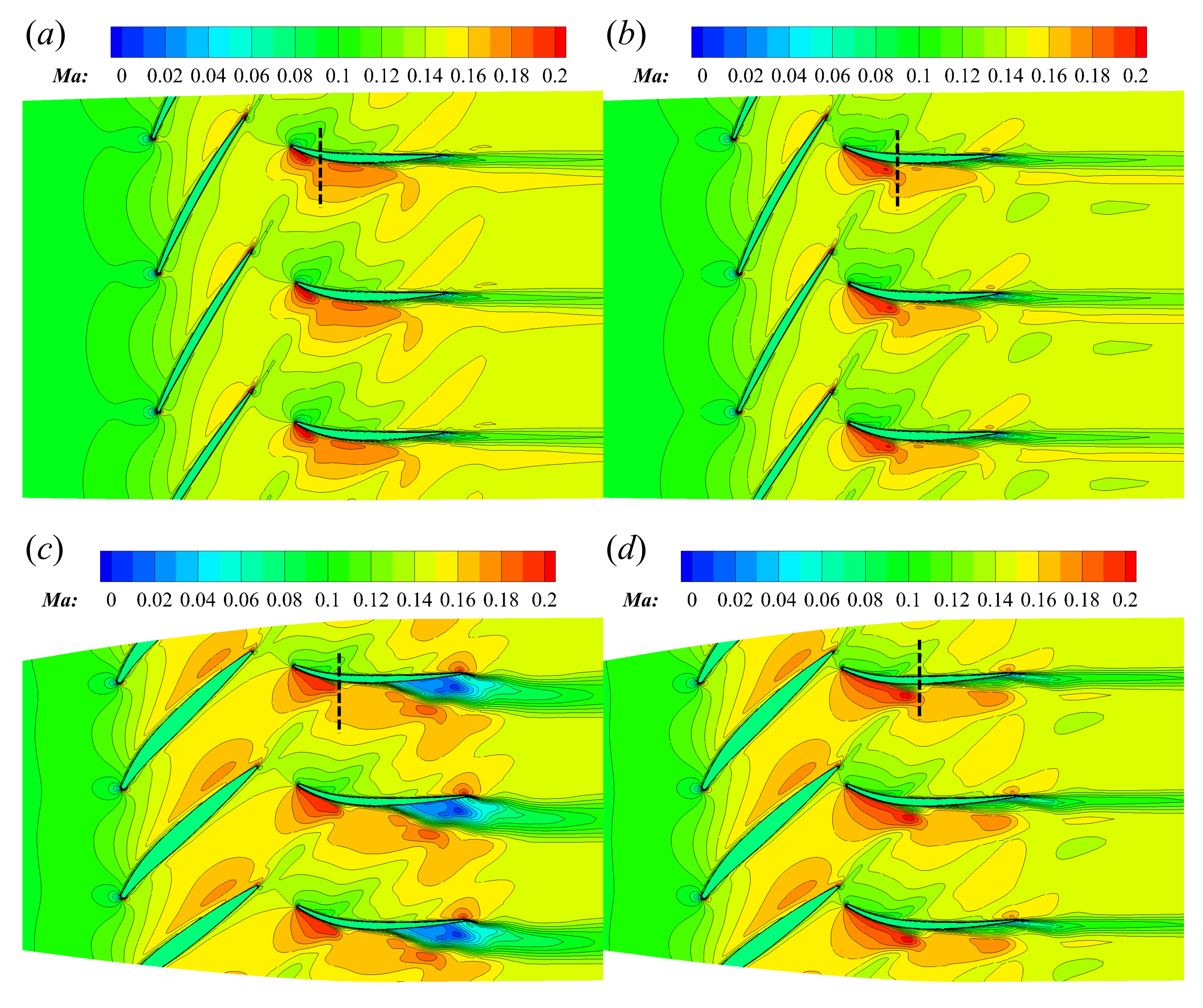
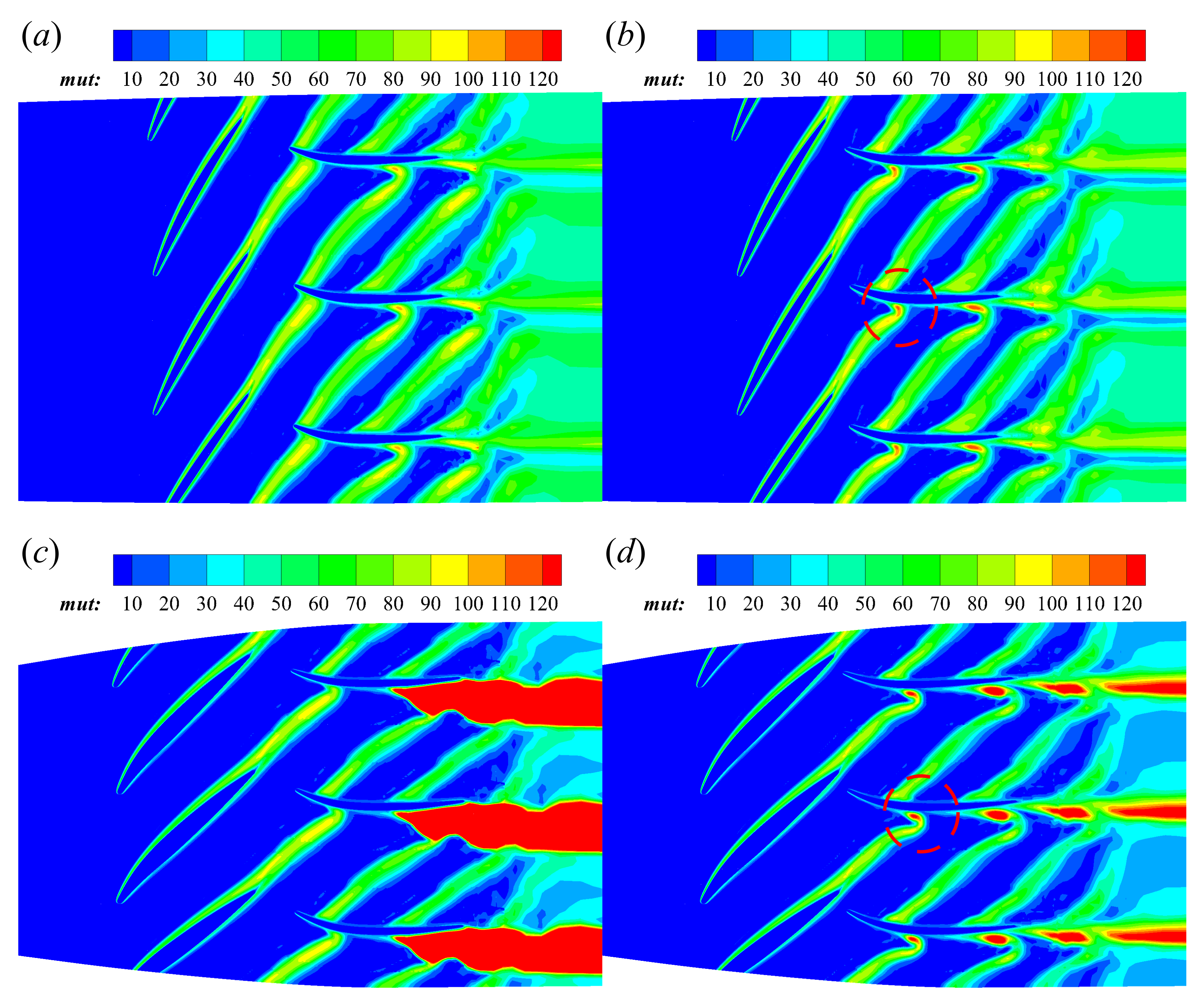
To explore the generation of performance enhancement from the two blade rows, Figure 16 and Figure 17 show the instantaneous distributions of Mach number and turbulence viscosity of the same moment for the two different gaps, respectively, at the same flow coefficient investigated. These flow contours were visualized on the and the span sections, as representatives for the shroud and the hub regions, respectively. As shown in the second column of Figure 16 and Figure 17, the flow contours at the extremely small gap were also smooth and did not suffer from the discontinuity generated by the blade–row interfaces encountered in the body-fitted approach, indicating that the IB method could be well applied to simulations of multi-row models with small gaps. For the two gaps, their flow characteristics on the span section seemed to be similar, see the comparisons of the first row in Figure 16 and Figure 17, respectively. When the gap was reduced, it was noticeable that higher turbulence intensity could be observed when the rotor wake impinged on the stator in the smaller-gap case at both the shroud and the hub regions, see the areas marked by the red dashed circles in Figure 17b,d. In the studies of Du et al. [10,11], it was found that when the gap was small, every time a rotor blade swept over a stator blade, a strong unsteady vortex shed from the trailing edge of the rotor blade, thus, increasing the oscillation amplitude as well as the mean value of the lift of the blade. Normally, flow turbulence intensity can be well enhanced by vortex structures as the magnitude of vorticity is part of the source term in the governing equation of the SA turbulence model. After the unsteady vortices shed from the rotor blade impinge on the downstream stator blade, the turbulence intensity might be further enhanced. On the other hand, higher velocity gradient was formed along the direction of the rotor wake when the gap was reduced, see the comparison of contours in Figure 16, which might also play a significant role in the increase of turbulence intensity of the rotor wake.
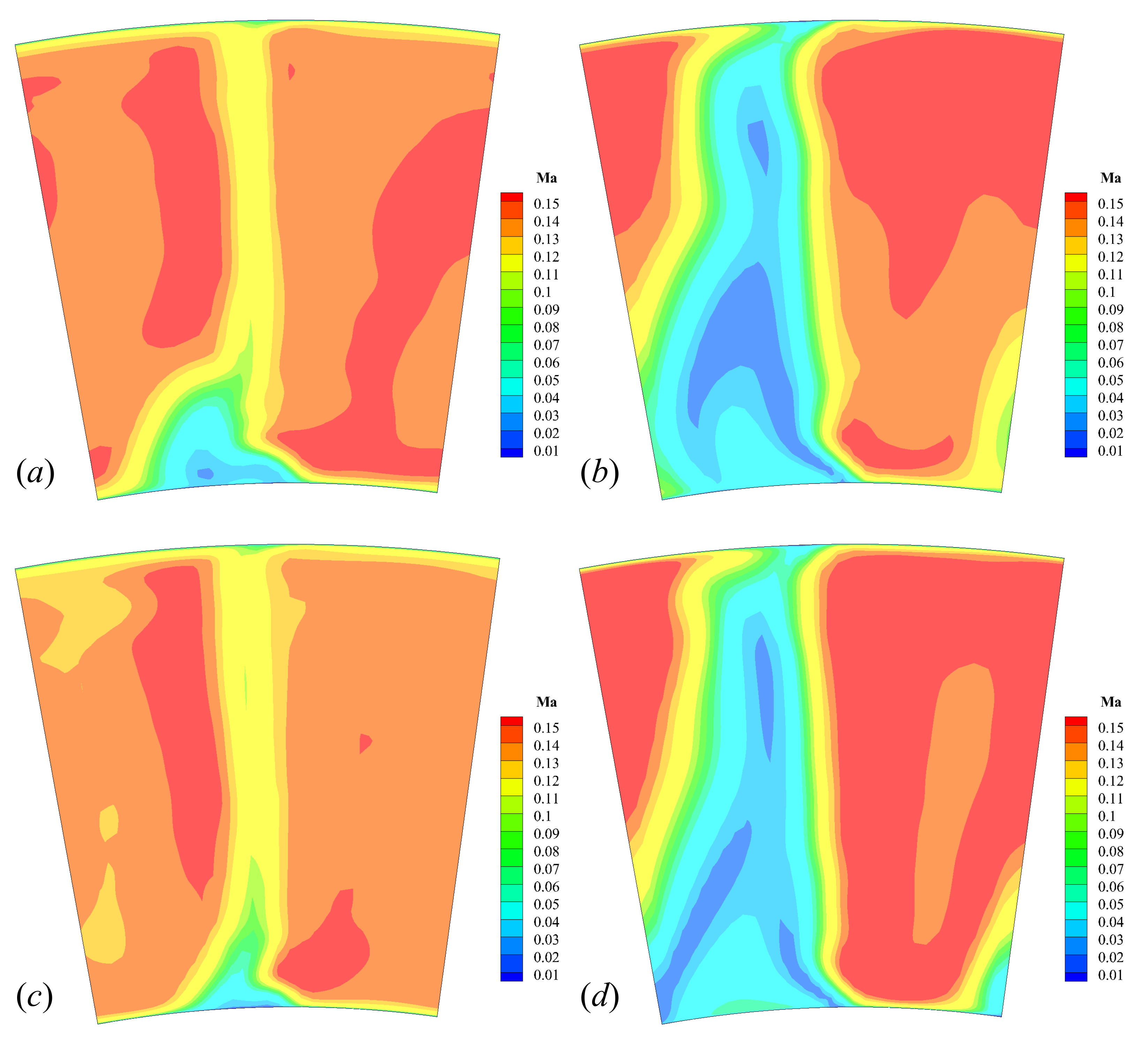
Figure 16 and Figure 17 show that the reduction of the gap greatly impacted the flow structures at the hub region. At the designed gap, flow separation could be observed in the stator hub, as shown in Figure 16c and Figure 17c. Such a phenomenon is widely encountered by high-loading compressors [51]. However, this separation is well suppressed in the smaller-gap case, as shown in Figure 16d and Figure 17d. As regards the authors’ acknowledgement, such an effect of reducing gap has not been reported yet in any experiment or simulation. This might be due to the fact that the smallest gaps considered in previous numerical studies, e.g., Hsu and Wo [16], Przytarski and Wheeler [17], were limited by the body-fitted grids and significantly larger than that of the present work. Figure 18 also shows the distributions of Ma at the two gaps on a downstream section to the stator’s trailing edge. Besides the case of , the contours at were also included, as a representative for the near-stall condition. It can be seen from Figure 18a,c, flow separation existed in a small region near the stator hub at and the reduction of the gap almost suppressed all the separation in the hub region. When the compressor worked at the near-stall point, although flow separation still existed in all span locations after the gap was reduced, both its width in pitch and the areas with the lowest Mach number were observed to shrink, as shown by the comparison of Figure 18b,d, indicating the effect of suppression to the flow separation still played a significant role at the near-stall condition after the gap reduced. It is known that RANS models always fail to accurately capture details of separated and tip leakage flows without additional modifications. However, the results in Figure 5a suggest that this inaccuracy was insignificant in the prediction of the compressor performance, as the numerical results did not exhibit much difference with the experimental data. Actually, RANS models are still widely used to study compressor flows. Although the flow separation in the stator was one major aspect of the present study, what we wanted to highlight was the dependence of this separation on the gap. The details of the separated flow, e.g., the spanwise length of the region with separation, obtained by the numerical study might be different from the reality, but the overall tendency observed with a reducing gap is still inspiring.
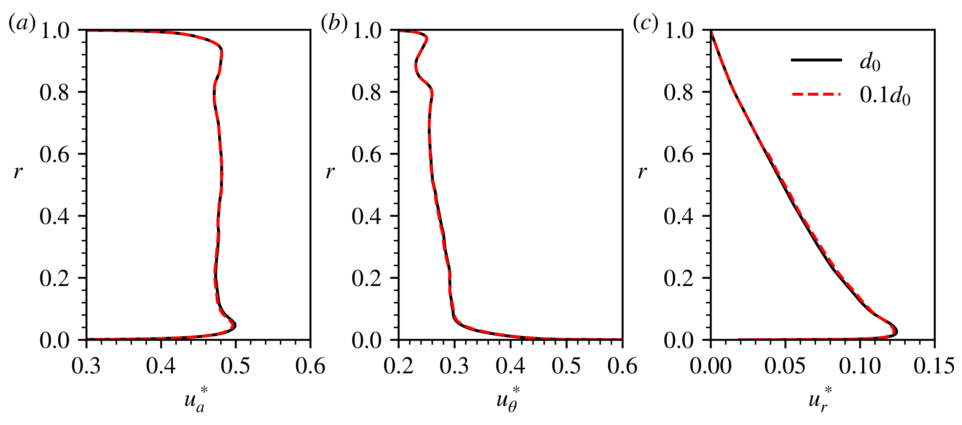
To further analyze the cause of suppression to the flow separation, the spanwise distributions of the flow velocity and static pressure on the outlets of the rotor and the stator were investigated. Figure 19 shows the spanwise distributions of the three non-dimensional velocity components on the rotor outlet at the two gaps. The reference for the velocity components shown in Figure 19 is . It can be seen that the three components almost remained the same in all span locations when the gap reduced, suggesting that the inlet-flow angles of the stator at the two gaps were also close to each other. Therefore, the suppression to the flow separation in the stator was not due to the change of the inlet-flow angle. It can be observed in Figure 14a that the total pressure rise at the hub region of rotor increased after the gap reduced. Since the velocity distributions on the rotor outlet at the two gaps were almost the same, it, thus, could be inferred that most of the increase of the total pressure was due to the rise of the static pressure on the rotor outlet.
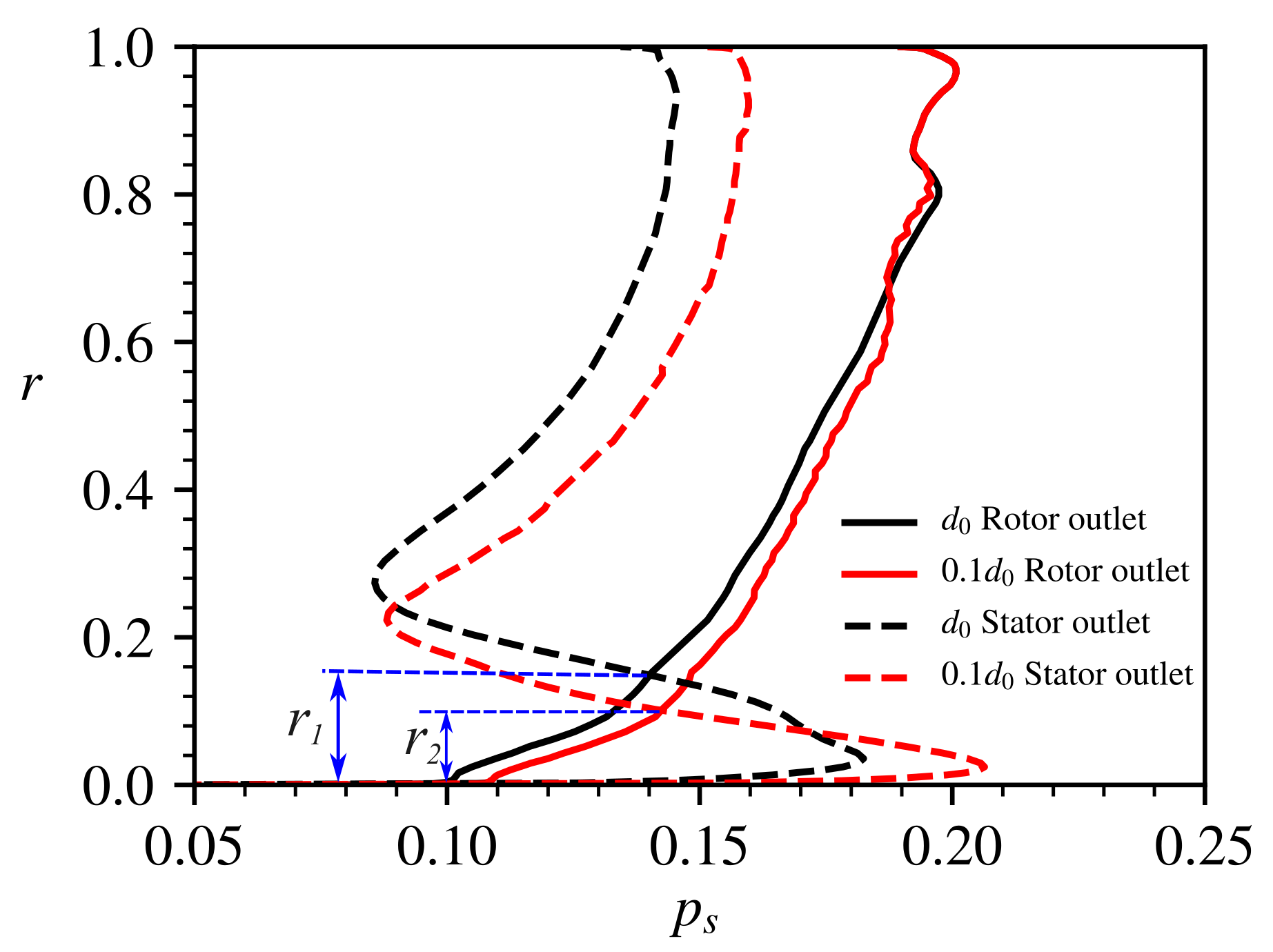
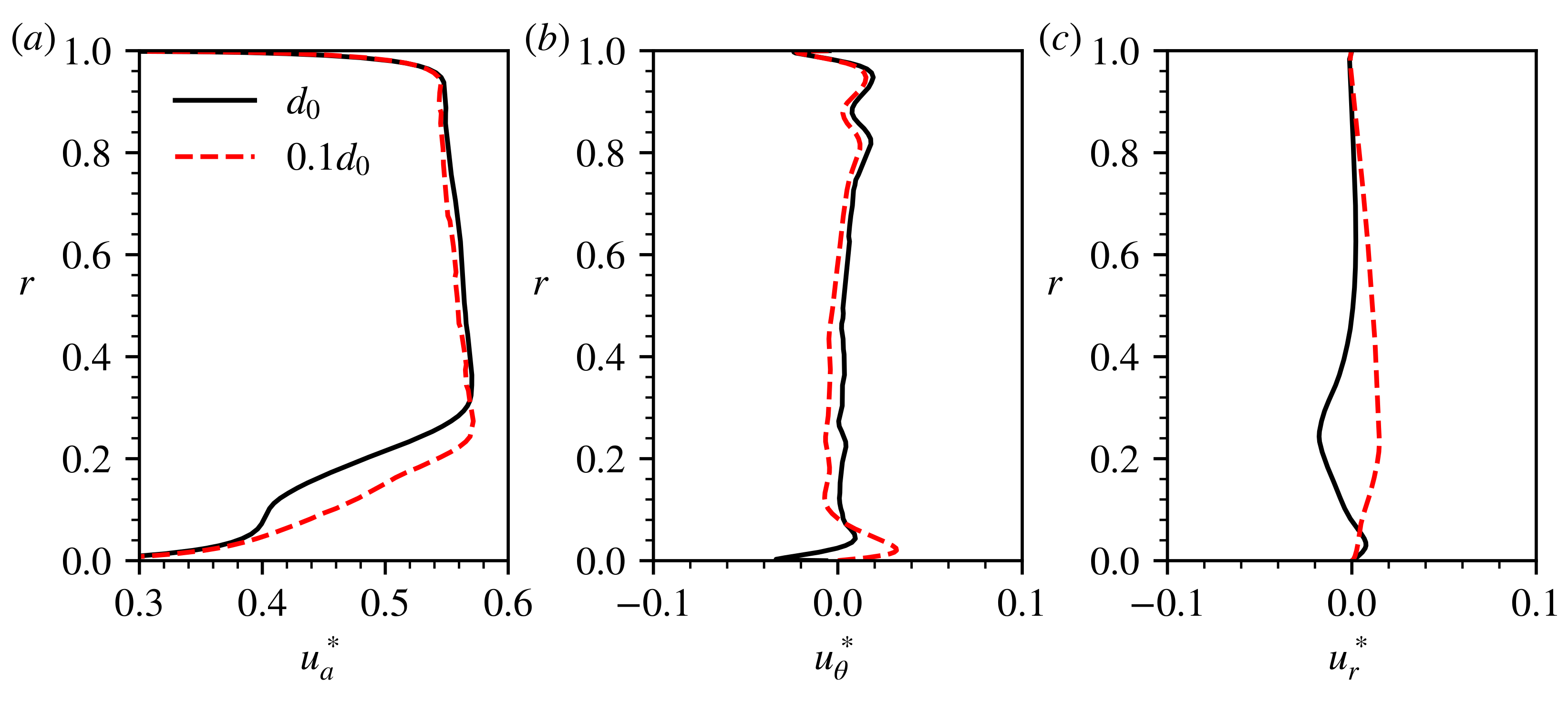
Figure 20 shows the spanwise distributions of the static pressure on the rotor and the stator outlet for the two gaps. It can be confirmed that the static pressure on the rotor outlet was found to increase in most span locations as the gap reduced. The difference between the static pressures on the inlet and the outlet of the stator in Figure 20 revealed that the flow experienced an adverse pressure gradient in the hub region of the stator, which was related to the separation. and in Figure 20 are used to denote the height in span of the region with adverse pressure gradient at and , respectively. Due to the increase of the static pressure in the stage gap after the gap reduced, the region with adverse pressure gradient was found to shrink, i.e., . This improvement compressed the separation region, thus, further reducing the total pressure loss in the stator hub region and resulting in a great enhancement to the performance of the stator. To further demonstrate the flow variation on the stator outlet, Figure 21 shows the spanwise distributions of the three velocity components on the stator outlet, which are normalized by . Prominent differences can be observed for the flow velocity near the hub, especially for the axial and the radial components in Figure 21a,c, respectively, and both the components were found to be higher in the smaller-gap case. These differences of flow velocity suggested that the mass flow rate increased in the stator hub region and the blockage caused by the flow separation improved. In addition, the circumferential components, shown in Figure 21b, were close to zero at all span locations at the designed gap, and only exhibited slight differences when the gap differed.
From Figure 19, Figure 20 and Figure 21 it can be found that over most of the span, the stator was accelerating the flow and decreasing the pressure, which was an unexpected behavior for a compressor stator. Normally, the stator of a compressor should both change the flow direction and increase the static pressure. However, for the present stator working in a low-speed compressor, it was designed mainly to change the flow direction with a very weak capacity of increasing the static pressure. As can be seen from Figure 4, the flow channel contracted along the axial direction. Therefore, the flow accelerated after it flowed out the rotor. Since the stator was designed to work at a high-loading state(i.e., high inlet flow angle, especially near the hub, see Figure 19, flow separation exited in the hub of the stator, resulting in a further decrease of the flow area in the stator. All these factors made the flow accelerate in the stator and the pressure thus decreased. For this condition, an obvious adverse pressure gradient was observed at the stator hub and reduced adverse pressure gradient could help to suppress the flow separation. Specifically, after the gap reduced and the flow separation was partly suppressed, the blockage at the hub region also improved, thus, resulting in a smaller decrease of static pressure in the stator passage, see the range of in Figure 20, and the increase of the axial flow velocity at the hub region, see Figure 21a. Note that reduction of the gap was achieved by moving the stator upstream, which made the channel contraction at the stator hub more important. This factor might also play a role in the flow suppression, and future studies are necessary to further demonstrate this effect.
The analysis in this section shows that both the rotor and the stator contribute to performance enhancement after the gap is reduced. At the smaller gap, the rotor outputs more work to the flow and increases the static pressure at the stage gap, which can improve the adverse pressure gradient and suppress the flow separation at the stator hub. The flow variation in the stator further reduces the total pressure loss at the hub and results in a great benefit to the stage performance. For the case considered in the present study, the performance increase of the stator resulted from two mechanisms: wake recovery, which is a classical manner to explain performance increase, and suppression to the stator flow separation, which is one major point of the present work. The first mechanism was observed in upper span locations, where the stator flow was attached, and the ratio of performance increase was less than that in the lower span range, where the second mechanism dominated. For a configuration without separation, when the gap reduced, the great benefit of suppressing separated flow did not exist and the performance increase of the stator should be similar with that in the upper span range of the present study. In this situation, only the mechanism of wake recovery affected the performance increase. However, for modern high-loading compressors, stator flow separation is common [51], and, therefore, the present conclusion can still be applied.
3.4. Unsteady Characteristics
Time profiles shown in Figure 13 exhibit more violent fluctuations when the gap was reduced. Increases of the fluctuations might deteriorate the aeroelastic and the aeroacoustic performances of the compressor. However, in experiments, it is challenging to measure the pressure fluctuation on a rotating blade and hard to know its distribution on the whole surface. Therefore, the effect of gap on the unsteady pressure on the blade surfaces was of interest to the present study.
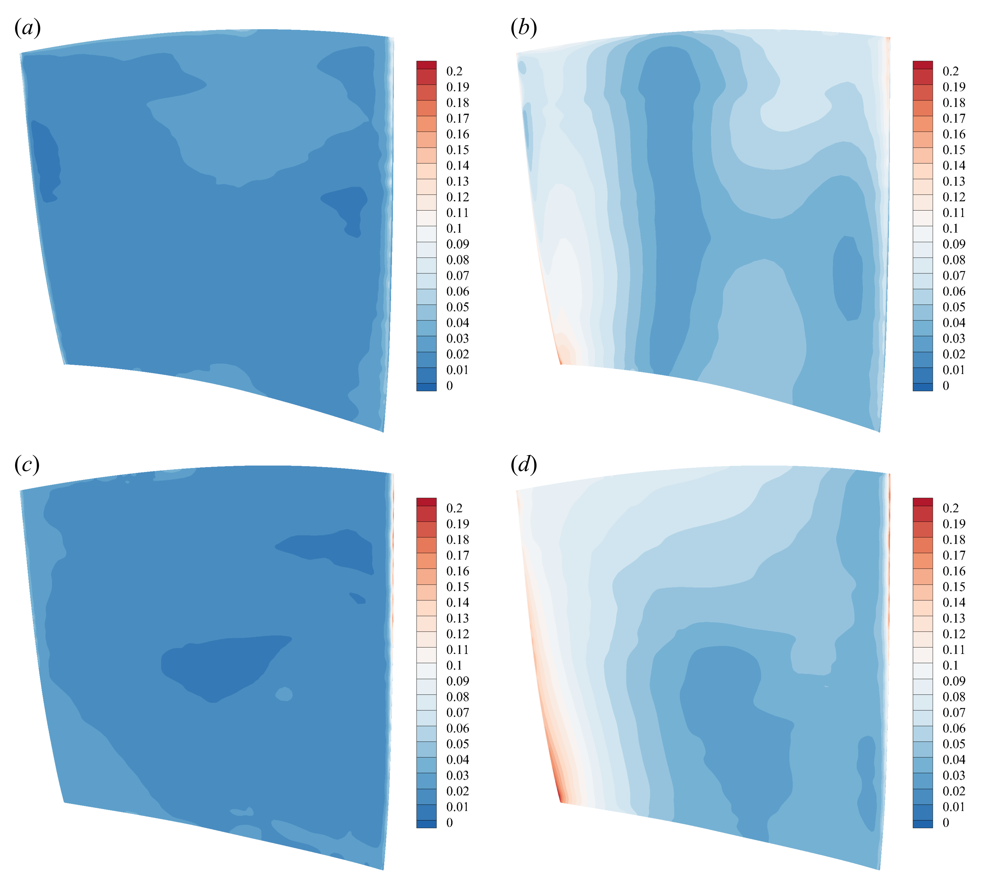
Figure 22 and Figure 23 show the distributions of the pressure fluctuation amplitude on the rotor and the stator, respectively, at the two gaps with . The amplitudes were quantified by half the peak-to-peak values for the unsteady pressures on the blade segments. Specifically, the rear part of the rotor blade suffered more from the fluctuation when the gap was reduced and the highest value was observed near the trailing edge. This fluctuation included the unsteady pressure generating on the stator and propagating upstream, and reduction of the gap not only strengthened the fluctuation on the stator, but also shortened the distance of attenuation, thus, highly increasing the amplitude of the unsteady pressure on the rotor blade. Przytarski and Wheeler [17] reported that the freestream turbulence levels rose significantly after the gap was reduced, which might also be related to the stronger fluctuation propagating upstream.
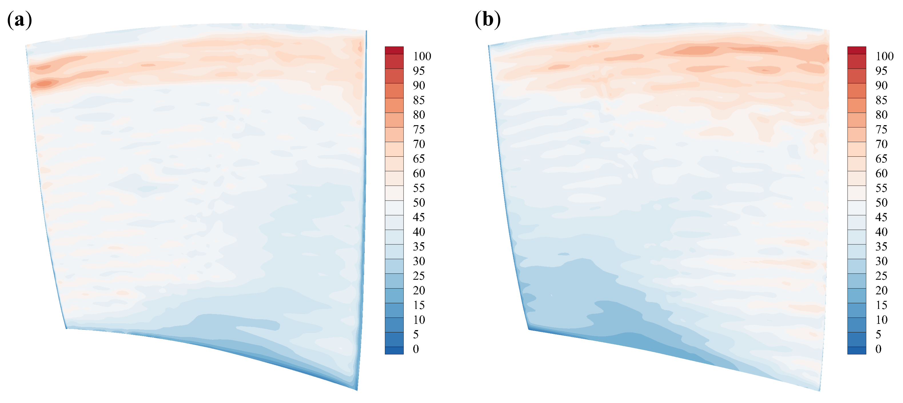
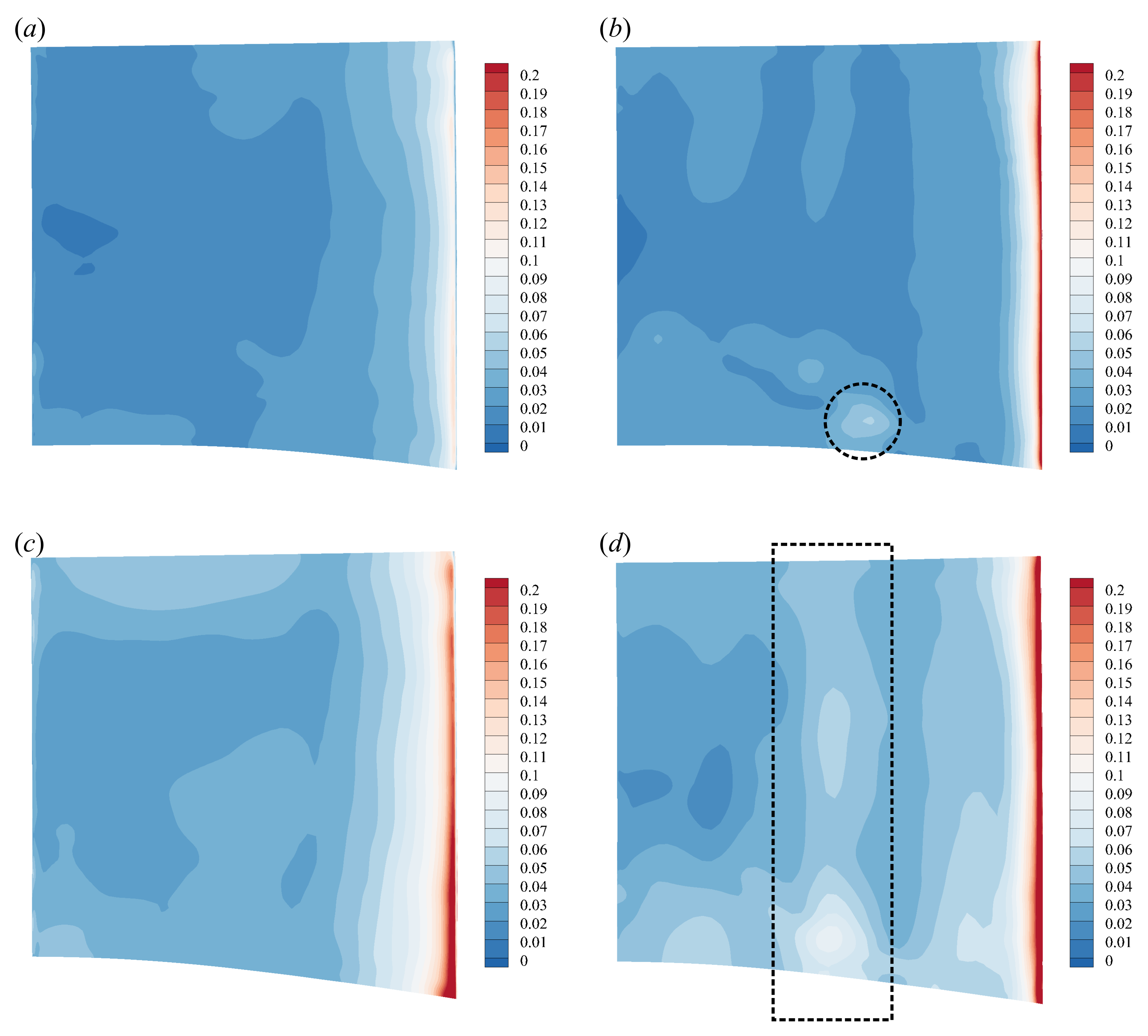
On the other hand, the aeroacoustic performance of the compressor depends on the flow characteristics of the stator. At the designed gap, only the leading-edge region of the stator exhibited pretty violent pressure fluctuation while the fluctuation was not obvious in most of the remaining regions, as shown by Figure 23a,b. After the gap was reduced, the fluctuation amplitudes were also found to increase on the whole stator, like the rotor. Specifically, the highest amplitude on the leading edge of the stator’s pressure side was more than twice the corresponding value at the designed gap, as can be identified from Figure 23a,c. The region with the highest fluctuation amplitude on the stator’s suction, i.e., the red areas at the leading edge in Figure 23b,d, was also found to expand toward the rear of the blade after the gap reduced. With the rotor passing, the leading edge of the stator chopped the rotor wake into two parts, resulting in violent fluctuation at this region, which also formed the main source of interaction noise.
In addition, at the designed gap, higher pressure fluctuation also existed near the mid-chord of the suction surface of the stator, as marked by the black dashed circle in Figure 23b. When the gap reduced, this region enlarged along the span as marked by the black dashed box in Figure 23d. This region with stronger fluctuation was well related to the interaction of the rotor wake and the stator flow. As can be found from the contours of Mach number in Figure 16, there was a region of flow acceleration near the leading edge of the suction surface of the stator, the end of which is marked by a dashed line in black. After the rotor wake was chopped by the stator, a new wake formed and evolved along the suction surface of the stator. Due to the interaction of the rotor wake and the stator flow, stronger pressure fluctuation then formed near the end of the acceleration region as a consequence, as revealed by Figure 23b,d. There was another small acceleration region downstream of that marked in Figure 16d on the suction surface of the stator and obvious pressure fluctuation could also be observed near it, as shown by Figure 23d. Therefore, in addition to the chop of rotor wake, the interaction of the rotor wake/stator flow was another main source of pressure fluctuation on the stator, and both of the two sources could be strongly enhanced by the reduction of the gap.
4. Conclusions
This paper presents the application of an Immersed Boundary method to study the effect of gap on the blade–row interaction for a low-speed single-stage compressor. The hybrid mesh strategy, together with the wall model and adaptive mesh refinement, facilitates the employment of the IB method for high Reynolds-number internal flows, also making the computational cost affordable. With the IB method, the two blade rows can be modeled in the same coordinate and the mesh can be easily constructed, even at an extremely small stage gap. The main finding of the present study is that reduction of the gap can both enhance the rotor loading and suppress the flow separation near the stator hub, thus, producing obvious performance benefit to the compressor.
Simulations were first conducted at the designed gap, , and overall performance showed good agreement with the experimental data. The numerical convergence was also carefully examined. Then, the gap was reduced to of the designed value, i.e., , and comparisons showed that the reduction of the gap increased the pressure rise on both the rotor and the stator outlets, and also reduced the total pressure loss of the stator, indicating both the two rows contributed to the performance enhancement. Further analysis revealed that the rotor worked at a higher-loading state, and thus resulted in the increase of the total pressure rise on the rotor outlet, when the gap was reduced. Such a variation of the total pressure rise was mainly contributed to by the increase of the static pressure on the rotor outlet, which could reduce the adverse pressure gradient at the hub region of the stator passage. Therefore, the flow separation in this region was also suppressed, which played a significant role in the performance increase of the stator.
The present work also proves the potential of the IB method in simulating the blade–row interaction at an extremely small gap, and future works will pay much attention to the validation of these new flow mechanisms through experimental studies.
Author Contributions
Conceptualization, Z.W.; Funding acquisition, X.S.; Investigation, Z.W. and L.D.; Methodology, L.D.; Supervision, X.S.; Validation, Z.W.; Writing—original draft, Z.W.; Writing—review and editing, L.D. and X.S. All authors have read and agreed to the published version of the manuscript.
Funding
This research was funded by the National Natural Science Foundation of China (grant Nos.51790514 and 52022009), the National Science and Technology Major Project (grant No. 2017-II-003-0015) and Key Laboratory Foundation (2021-JCJQ-LB-062-0102).
Institutional Review Board Statement
Not applicable.
Informed Consent Statement
Not applicable.
Data Availability Statement
Not applicable.
Conflicts of Interest
The authors declare no conflict of interest.
References
- Smith, L.H. Casing Boundary Layers in Multistage Axial Flow Compressors. In Flow Research on Blading; Dzung, L.S., Ed.; Elsevier Publishing Company: Amsterdam, The Netherlands, 1970. [Google Scholar]
- Mikolajczal, A.A. The Practical Importance of Unsteady Flow in AGARD CP-177, Unsteady Phenomena in Turbomachinary; Technical Report; Swiss Federal Institute of Technology: Zürich, Switzerland, 1977. [Google Scholar]
- Smith, L. Wake Dispersion in Turbomachines. J. Basic Eng. 1966, 88, 688–690. [Google Scholar] [CrossRef]
- Adamczyk, J.J. Wake mixing in axial flow compressors. In Proceedings of the International Gas Turbine and Aeroengine Congress and Exhibition, Birmingham, UK, 10–13 June 1996. [Google Scholar] [CrossRef] [Green Version]
- Deregel, P.; Tan, C. Impact of Rotor Wakes on Steady-State Axial Compressor Performance. In Proceedings of the ASME 1996 International Gas Turbine and Aeroengine Congress and Exhibition, Birmingham, UK, 10–13 June 1996; Volume 1. [Google Scholar]
- Gorrell, S.E.; Copenhaver, W.W.; Chriss, R.M. Upstream wake influences on the measured performance of a transonic compressor stage. J. Propuls. Power 2001, 17, 43–48. [Google Scholar] [CrossRef]
- Gorrell, S.E.; Okiishi, T.H.; Copenhaver, W.W. Stator-rotor interactions in a transonic compressor—Part 1: Effect of blade-row spacing on performance. J. Turbomach. 2003, 125, 328–335. [Google Scholar] [CrossRef]
- Nolan, S.P.; Botros, B.B.; Tan, C.S.; Adamczyk, J.J.; Greitzer, E.M.; Gorrell, S.E. Effects of upstream wake phasing on transonic axial compressor performance. J. Turbomach. 2011, 133, 021010. [Google Scholar] [CrossRef]
- Clark, K.P.; Gorrell, S.E. Analysis and prediction of shock-induced vortex circulation in transonic compressors. J. Turbomach. 2015, 137, 121007. [Google Scholar] [CrossRef]
- Du, L.; Sun, X.; Yang, V. Generation of vortex lift through reduction of rotor/stator gap in turbomachinery. J. Propuls. Power 2016, 32, 472–485. [Google Scholar] [CrossRef] [Green Version]
- Du, L.; Sun, X.; Yang, V. Vortex-lift mechanism in axial turbomachinery with periodically pitched stators. J. Propuls. Power 2016, 32, 486–499. [Google Scholar] [CrossRef] [Green Version]
- Xu, H.; Jin, D.; Wang, M.; Du, L.; Sun, D.; Gui, X.; Sun, X. High blade lift generation through short rotor–stator axial spacing in a tiny pump. Aerosp. Sci. Technol. 2018, 79, 328–335. [Google Scholar] [CrossRef]
- Rai, M.M. Navier-stokes simulations of rotor-stator interaction using patched and overlaid grids. J. Propuls. Power 1987, 3, 387–396. [Google Scholar] [CrossRef]
- Jorgenson, P.C.; Chima, R.V. Explicit Runge-Kutta method for unsteady rotor/stator interaction. AIAA J. 1989, 27, 743–749. [Google Scholar] [CrossRef]
- Giles, M.B. Stator/rotor interaction in a transonic turbine. J. Propuls. Power 1990, 6, 621–627. [Google Scholar] [CrossRef]
- Hsu, S.T.; Wo, A.M. Reduction of Unsteady Blade Loading by Beneficial Use of Vortical and Potential Disturbances in an Axial Compressor With Rotor Clocking. J. Turbomach. 1998, 120, 705–713. [Google Scholar] [CrossRef]
- Przytarski, P.J.; Wheeler, A.P. The effect of gapping on compressor performance. J. Turbomach. 2020, 142, 121006. [Google Scholar] [CrossRef]
- Peskin, C.S. The immersed boundary method. Acta Numer. 2002, 11, 479–517. [Google Scholar] [CrossRef] [Green Version]
- Mittal, R.; Iaccarino, G. Immersed boundary methods. Annu. Rev. Fluid Mech. 2005, 37, 239–261. [Google Scholar] [CrossRef] [Green Version]
- Griffith, B.E.; Patankar, N.A. Immersed Methods for Fluid-Structure Interaction. Annu. Rev. Fluid Mech. 2020, 52, 421–448. [Google Scholar] [CrossRef] [Green Version]
- Zhong, G.; Sun, X. New simulation strategy for an oscillating cascade in turbomachinery using immersed-boundary method. J. Propuls. Power 2009, 25, 312–321. [Google Scholar] [CrossRef]
- Chen, C.; Wang, Z.; Du, L.; Sun, D.; Sun, X. Simulating unsteady flows in a compressor using immersed boundary method with turbulent wall model. Aerosp. Sci. Technol. 2021, 115, 106834. [Google Scholar] [CrossRef]
- Cheng, L.; Du, L.; Wang, X.; Sun, X. Inviscid Nonlinear Modeling of Vibration-Induced Acoustic Resonance of a Linear Cascade. AIAA J. 2021, 59, 1849–1860. [Google Scholar] [CrossRef]
- Roma, A.M.; Peskin, C.S.; Berger, M.J. An Adaptive Version of the Immersed Boundary Method. J. Comput. Phys. 1999, 153, 509–534. [Google Scholar] [CrossRef] [Green Version]
- Vanella, M.; Rabenold, P.; Balaras, E. A direct-forcing embedded-boundary method with adaptive mesh refinement for fluid-structure interaction problems. J. Comput. Phys. 2010, 229, 6427–6449. [Google Scholar] [CrossRef]
- Angelidis, D.; Chawdhary, S.; Sotiropoulos, F. Unstructured Cartesian refinement with sharp interface immersed boundary method for 3D unsteady incompressible flows. J. Comput. Phys. 2016, 325, 272–300. [Google Scholar] [CrossRef] [Green Version]
- Al-Marouf, M.; Samtaney, R. A versatile embedded boundary adaptive mesh method for compressible flow in complex geometry. J. Comput. Phys. 2017, 337, 339–378. [Google Scholar] [CrossRef] [Green Version]
- Wang, Z.; Du, L.; Sun, X. Adaptive mesh refinement for simulating fluid-structure interaction using a sharp interface immersed boundary method. Int. J. Numer. Methods Fluids 2020, 92, 1890–1913. [Google Scholar] [CrossRef]
- Capizzano, F. Turbulent wall model for immersed boundary methods. AIAA J. 2011, 49, 2367–2381. [Google Scholar] [CrossRef]
- Capizzano, F. Coupling a wall diffusion model with an immersed boundary technique. AIAA J. 2016, 54, 728–734. [Google Scholar] [CrossRef]
- Tamaki, Y.; Harada, M.; Imamura, T. Near-wall modification of Spalart-Allmaras turbulence model for immersed boundary method. AIAA J. 2017, 55, 3027–3039. [Google Scholar] [CrossRef]
- Berger, M.J.; Aftosmis, M.J. An ODE-based wall model for turbulent flow simulations. AIAA J. 2018, 56, 700–714. [Google Scholar] [CrossRef]
- Cai, S.G.; Degrigny, J.; Boussuge, J.F.; Sagaut, P. Coupling of turbulence wall models and immersed boundaries on Cartesian grids. J. Comput. Phys. 2021, 429, 109995. [Google Scholar] [CrossRef]
- Constant, B.; Péron, S.; Beaugendre, H.; Benoit, C. An improved immersed boundary method for turbulent flow simulations on Cartesian grids. J. Comput. Phys. 2021, 435, 110240. [Google Scholar] [CrossRef]
- Dong, X.; Sun, D.; Li, F.; Jin, D.; Gui, X.; Sun, X. Effects of rotating inlet distortion on compressor stability with stall precursor-suppressed casing treatment. J. Fluids Eng. Trans. ASME 2015, 137, 111101. [Google Scholar] [CrossRef]
- Li, F.; Li, J.; Dong, X.; Zhou, Y.; Sun, D.; Sun, X. Stall-warning approach based on aeroacoustic principle. J. Propuls. Power 2016, 32, 1353–1364. [Google Scholar] [CrossRef]
- Dong, X.; Sun, D.; Li, F.; Jin, D.; Gui, X.; Sun, X. Effects of Stall Precursor-Suppressed Casing Treatment on a Low-Speed Compressor with Swirl Distortion. J. Fluids Eng. Trans. ASME 2018, 140, 091101. [Google Scholar] [CrossRef]
- Dong, X.; Li, F.; Xu, R.; Sun, D.; Sun, X. Further investigation on acoustic stall-warning approach in compressors. J. Turbomach. 2019, 141, 061001. [Google Scholar] [CrossRef]
- Xu, D.; He, C.; Sun, D.; Sun, X. Stall inception prediction of axial compressors with radial inlet distortions. Aerosp. Sci. Technol. 2021, 109, 106433. [Google Scholar] [CrossRef]
- Spalart, P.R.; Allmaras, S.R. A one-equation turbulence model for aerodynamic flows. In Proceedings of the 30th Aerospace Sciences Meeting and Exhibit, Reno, NV, USA, 6–9 January 1992. [Google Scholar] [CrossRef]
- Roe, P.L. Approximate Riemann Solvers, Parameter Vectors, and Difference Schemes. J. Comput. Phys. 1981, 43, 357–372. [Google Scholar] [CrossRef]
- Li, X.; Gu, C. An All-Speed Roe-type scheme and its asymptotic analysis of low Mach number behaviour. J. Comput. Phys. 2008, 227, 5144–5159. [Google Scholar] [CrossRef]
- Van Leer, B. Towards the Ultimate Conservative Difference Scheme. V. A Second-Order Sequel to Godunov’s Method. J. Comput. Phys. 1979, 32, 101–136. [Google Scholar] [CrossRef]
- Berger, M.J.; Oliger, J. Adaptive mesh refinement for hyperbolic partial differential equations. J. Comput. Phys. 1984, 53, 484–512. [Google Scholar] [CrossRef]
- Berger, M.J.; Colella, P. Local Adaptive Mesh Refinement for Shock Hydrodynamics. J. Comput. Phys. 1989, 82, 64–84. [Google Scholar] [CrossRef] [Green Version]
- Aftosmis, M.J.; Melton, J.E.; Berger, M.J. Adaptation and surface modeling for Cartesian mesh methods. In Proceedings of the 12th Computational Fluid Dynamics Conference, San Diego, CA, USA, 19–22 June 1995. [Google Scholar] [CrossRef]
- Gilmanov, A.; Sotiropoulos, F.; Balaras, E. A general reconstruction algorithm for simulating flows with complex 3D immersed boundaries on Cartersian grids. J. Comput. Phys. 2003, 191, 660–669. [Google Scholar] [CrossRef]
- Gilmanov, A.; Sotiropoulos, F. A hybrid Cartesian/immersed boundary method for simulating flows with 3D, geometrically complex, moving bodies. J. Comput. Phys. 2005, 207, 457–492. [Google Scholar] [CrossRef]
- Spalding, D.B. A single formula for the “law of the wall”. J. Appl. Mech. Trans. ASME 1961, 28, 455–457. [Google Scholar] [CrossRef]
- Chung, M.; Wo, A.M. Navier-Stokes and Potential Calculations of Axial Spacing Effect on Vortical and Potential Disturbances and Gust Response in an Axial Compressor. J. Turbomach. 1997, 119, 472–481. [Google Scholar] [CrossRef]
- Dickens, T.; Day, I. The design of highly loaded axial compressors. J. Turbomach. 2011, 133, 031007. [Google Scholar] [CrossRef]
Figure 1.
Grid strategies to a turbomachinery problem: (a) Cartesian grid, (b) channel-conformal structured grid, (c) multi-level mesh with AMR. The red solid lines represent the channel, and both the black solid circles in (a,b) and the black solid line in (c) represent the blades inside the channel.

Figure 2.
Cell classification for the curvilinear grid near the wall.

Figure 3.
A same forcing distance is used for different wall orientations.

Figure 4.
Grid used in the simulations of rotor/stator interaction: (a) the background (first-level) grid for the flow channel, and (b) part of the multi-level grid with AMR to the blade locations.
Figure 4.
Grid used in the simulations of rotor/stator interaction: (a) the background (first-level) grid for the flow channel, and (b) part of the multi-level grid with AMR to the blade locations.

Figure 5.
Comparison of the performance obtained by the experiment and the present IB method with different numbers of refinement level: (a) Static-to-total pressure rise coefficient; (b) adiabatic efficiency.
Figure 5.
Comparison of the performance obtained by the experiment and the present IB method with different numbers of refinement level: (a) Static-to-total pressure rise coefficient; (b) adiabatic efficiency.

Figure 6.
Error ratios of flow coefficients, total-to-total pressure rises and efficiencies compared to the reference data.
Figure 6.
Error ratios of flow coefficients, total-to-total pressure rises and efficiencies compared to the reference data.

Figure 7.
Unsteady pressure obtained by using different numbers of refinement level.

Figure 8.
Distributions of on the rotor blade. (a) Pressure surface and (b) suction surface.

Figure 9.
The relative positions of the rotor and the stator at: (a) and (b) .

Figure 10.
A close view to the 5-level mesh on the hub surface at .

Figure 11.
Aerodynamic performance at two row gaps: (a) the total-to-total pressure rise coefficient and (b) the adiabatic efficiency.
Figure 11.
Aerodynamic performance at two row gaps: (a) the total-to-total pressure rise coefficient and (b) the adiabatic efficiency.

Figure 12.
Aerodynamic performance at different row gaps with a fixed back pressure: (a) mass flow rate, (b) total pressure rise coefficient and (c) adiabatic efficiency.
Figure 12.
Aerodynamic performance at different row gaps with a fixed back pressure: (a) mass flow rate, (b) total pressure rise coefficient and (c) adiabatic efficiency.

Figure 13.
Time profiles of (a) the total pressure rise coefficient on the rotor outlet, (b) the aerodynamic moment on the rotor blade and (c) the total pressure rise coefficient on the stator outlet.
Figure 13.
Time profiles of (a) the total pressure rise coefficient on the rotor outlet, (b) the aerodynamic moment on the rotor blade and (c) the total pressure rise coefficient on the stator outlet.

Figure 14.
Spanwise distributions of the total pressure rise on (a) the rotor and (b) the stator outlets.
Figure 14.
Spanwise distributions of the total pressure rise on (a) the rotor and (b) the stator outlets.

Figure 15.
Spanwise distributions of (a) the incremental ratio of the total pressure rise on the rotor and the stator outlets when the gap reduced from to and (b) the total pressure loss coefficient of the stator at the two gaps.
Figure 15.
Spanwise distributions of (a) the incremental ratio of the total pressure rise on the rotor and the stator outlets when the gap reduced from to and (b) the total pressure loss coefficient of the stator at the two gaps.

Figure 16.
Flow contours of Ma on two span sections at for the two gaps: (a) 90% span and ; (b) 90% span and ; (c) 20% span and ; (d) 20% span and .
Figure 16.
Flow contours of Ma on two span sections at for the two gaps: (a) 90% span and ; (b) 90% span and ; (c) 20% span and ; (d) 20% span and .

Figure 17.
Flow contours of turbulence viscosity on two span sections at for the two gaps: (a) 90% span and ; (b) 90% span and ; (c) 20% span and ; (d) 20% span and .
Figure 17.
Flow contours of turbulence viscosity on two span sections at for the two gaps: (a) 90% span and ; (b) 90% span and ; (c) 20% span and ; (d) 20% span and .

Figure 18.
Distributions of Ma at the downstream section to the stator’s trailing edge: (a) and ; (b) and ; (c) and ; (d) and .
Figure 18.
Distributions of Ma at the downstream section to the stator’s trailing edge: (a) and ; (b) and ; (c) and ; (d) and .

Figure 19.
Spanwise distributions of the three velocity components on the rotor outlet at different stage gaps: (a) axial; (b) circumferential; (c) radial.
Figure 19.
Spanwise distributions of the three velocity components on the rotor outlet at different stage gaps: (a) axial; (b) circumferential; (c) radial.

Figure 20.
Spanwise distributions of the static pressure on the rotor and the stator outlets at different stage gaps.
Figure 20.
Spanwise distributions of the static pressure on the rotor and the stator outlets at different stage gaps.

Figure 21.
Spanwise distributions of the three velocity components on the stator outlet at different stage gaps: (a) axial; (b) circumferential; (c) radial.
Figure 21.
Spanwise distributions of the three velocity components on the stator outlet at different stage gaps: (a) axial; (b) circumferential; (c) radial.

Figure 22.
Distributions of the pressure fluctuation amplitude on the rotor blade. (a) , pressure surface, (b) , suction surface, (c) , pressure surface, (d) , suction surface.
Figure 22.
Distributions of the pressure fluctuation amplitude on the rotor blade. (a) , pressure surface, (b) , suction surface, (c) , pressure surface, (d) , suction surface.

Figure 23.
Distributions of the pressure fluctuation amplitude on the stator blade. (a) , pressure surface, (b) , suction surface, (c) , pressure surface, (d) , suction surface.
Figure 23.
Distributions of the pressure fluctuation amplitude on the stator blade. (a) , pressure surface, (b) , suction surface, (c) , pressure surface, (d) , suction surface.


Table 1.
Critical distances for different grid levels.
| Grid Level | Critical Distance (Normalized by c) |
|---|---|
| Level 1 | 0.18 |
| Level 2 | 0.07 |
| Level 3 | 0.03 |
| Level 4 | 0.01 |
| Level 5 | 0.007 |
Table 2.
Total cell numbers of the grids with different numbers of refinement level.
| Mesh | Total Cell Number |
|---|---|
| IB-3 | 2.91 millions |
| IB-4 | 5.80 millions |
| IB-5 | 9.66 millions |
| IB-6 | 22.83 millions |
Table 3.
Mass flow rates on the inlet and the outlets at different operation conditions obtained by the IB-5 grid.
Table 3.
Mass flow rates on the inlet and the outlets at different operation conditions obtained by the IB-5 grid.
| Operation Condition | Inlet | Outlet | Difference/Inlet |
|---|---|---|---|
| 1 | 0.340 | 0.342 | 0.59% |
| 2 | 0.329 | 0.328 | 0.30% |
| 3 | 0.316 | 0.315 | 0.32% |
| 4 | 0.302 | 0.303 | 0.33% |
| 5 | 0.286 | 0.286 | 0% |
| 6 | 0.266 | 0.265 | 0.37% |
| 7 | 0.242 | 0.240 | 0.83% |
Table 4.
R.M.S values of the unsteady pressure shown in Figure 7 and their error ratios to the reference data.
Table 4.
R.M.S values of the unsteady pressure shown in Figure 7 and their error ratios to the reference data.
| Mesh | R.M.S | Error Ratio |
|---|---|---|
| IB-3 | 0.3730 | 0.0652 |
| IB-4 | 0.3851 | 0.0348 |
| IB-5 | 0.4003 | 0.0032 |
| IB-6 | 0.3990 | reference |
Disclaimer/Publisher’s Note: The statements, opinions and data contained in all publications are solely those of the individual author(s) and contributor(s) and not of MDPI and/or the editor(s). MDPI and/or the editor(s) disclaim responsibility for any injury to people or property resulting from any ideas, methods, instructions or products referred to in the content. |
© 2023 by the authors. Licensee MDPI, Basel, Switzerland. This article is an open access article distributed under the terms and conditions of the Creative Commons Attribution (CC BY-NC-ND) license (https://creativecommons.org/licenses/by-nc-nd/4.0/).
Share and Cite
MDPI and ACS Style
Wang, Z.; Du, L.; Sun, X. Enhancement of Rotor Loading and Suppression of Stator Separation through Reduction of the Blade–Row Gap. Int. J. Turbomach. Propuls. Power 2023, 8, 6. https://doi.org/10.3390/ijtpp8010006
AMA Style
Wang Z, Du L, Sun X. Enhancement of Rotor Loading and Suppression of Stator Separation through Reduction of the Blade–Row Gap. International Journal of Turbomachinery, Propulsion and Power. 2023; 8(1):6. https://doi.org/10.3390/ijtpp8010006
Chicago/Turabian StyleWang, Zhuo, Lin Du, and Xiaofeng Sun. 2023. "Enhancement of Rotor Loading and Suppression of Stator Separation through Reduction of the Blade–Row Gap" International Journal of Turbomachinery, Propulsion and Power 8, no. 1: 6. https://doi.org/10.3390/ijtpp8010006