Numerical Determination of the Equivalent Sand Roughness of a Turbopump’s Surface and Its Roughness Influence on the Pump Characteristics

Abstract

The correct computation of flows over rough surfaces in technical systems, such as in turbomachines, is a significant issue for proper simulations of their performance data. Once the flow over rough surfaces is adequately computed in these machines, simulations become more trustworthy and can replace experimental prototyping. Roughness modelling approaches are often implemented in a solver to account for roughness effects in flow simulations. In these approaches, the equivalent sand roughness $k_s$ must be defined as a characteristic parameter of the rough surface. However, it is difficult to determine the corresponding $k_s$-value for a surface roughness. In this context, this paper shows a novel and time-efficient numerical method, the discrete porosity method (DPM), which can be used to determine the $k_s$-value of a rough surface. Applying this method, channel flow simulations were performed with an irregularly distributed cast iron surface from a turbopumps volute. After identifying the fully rough regime, the equivalent sand roughness was determined and a match with $k_s$-values from literature data was found. Subsequently, the established $k_s$-value for cast iron was used in a turbopump simulation with rough walls. The performance data of the pump were validated by experiments and a good agreement between the experimental and simulated performance data was found.

1. Introduction

Nowadays, flow simulations are widely used for design optimizations of turbomachines, such as for turbopumps, compressors, or turbines. Manufacturers strive to improve and customise the performance data of these machines through simulations, since they allow a cost-effective and comprehensive understanding of the flow physics in the systems.

Most flow simulations of such machines assume the surface to be hydraulically smooth [1]. This contradicts real flows in these machines, where every surface has a certain degree of roughness. The roughness effects can significantly influence the performance data of the turbomachine’s simulation. This is especially the case for turbopumps with low specific speeds $n_s$ (Equation (1)), which means that the machines are designed to deliver high-pressure heads $H_p=\Delta p_{tot}/\left(\rho g\right)$ at small flow rates Q (a nomenclature can be found at the end of this paper). Those pumps are characterised by long and narrow impeller channels and even narrower side chambers between the impeller and the housing. Both geometric features can lead to dominant roughness effects in the pump.

Juckelandt et al. [2] demonstrated a significant deviation between the simulated and experimentally assessed performance data of a radial turbopump with low specific speed. As can be seen in Figure 1, the inner efficiency ${\eta }_i$ (defined in Equation (13)) is monotonously overestimated in the pump simulation by an offset of $+10\%$. The authors stated the unconsidered wall roughness as the critical aspect in their simulations. This discrepancy may cause designers to favor experimental methods over simulations. Hence, an appropriate wall treatment with consideration of roughness modelling is crucial for the simulations in turbopumps with low specific speeds.

$$n_s=n·\frac{\sqrt{Q}}{H_p^{3/4}}$$

(1)

In this context, the state-of-the-art roughness modelling for simulations depend on the equivalent sand grain roughness $k_s$ as the characteristic standard to determine the impact of roughness effects [3]. According to Schlichting [4], the theory of equivalent sand grain roughness simplifies an arbitrary surface roughness to closely packed spheres, both having identical physical effects on the flow in the fully rough regime.

$$u^{+}=1/\kappa ln\left(y^{+}\right)+B-\Delta u^{+}\left(k_s^{+}\right)$$

(2)

It is well known that the dimensionless velocity profile $u^{+}=f\left(y^{+}\right)$ indicates a downshift $\Delta u^{+}$ at rough walls compared to the velocity profile in hydraulically smooth boundary layers [5], see Figure 2. Equation (2) applies for the logarithmic wall region, where the downshift $\Delta u^{+}$ is described as a function of the dimensionless equivalent sand grain roughness $k_s^{+}$ [6,7]. In Equation (2), the constants were experimentally determined as $\kappa =0.41$ and $B=5.0$ [3].

The roughness modelling in simulations, e.g., in turbomachines, is realised by considering this downshift $\Delta u^{+}\left(k_s^{+}\right)$ in the simulated velocity profile. This approach is called the modified logarithmic law-of-the-wall and it is one of the most common approaches to model the roughness effects. Roughness modelling approaches, which are based on the modified law-of-the-wall, were proposed by Refs. [8,9,10]. Alternatively, the roughness effects in a flow simulation of a turbomachine can also be modelled by changing the boundary conditions for turbulence variables near the rough wall, as proposed by Wilcox or Knopp et al. [11,12].

All of these approaches have in common that $k_s$ of the rough surface has to be defined, so that the effect of roughness can be properly computed by the modelling approach. However, it is still complicated to define the appropriate $k_s$ for surfaces with irregularly distributed roughness heights. Such surfaces are present, for example, at the unprocessed cast iron walls in the volute, impeller, or side chambers of a turbomachine [2].

Various experimental studies, which define the equivalent sand roughness for cast iron, can be found in the literature (

Table 1. Literature values for the equivalent sand grain roughness $k_s$ of new cast iron surfaces.

Reference	${\mathit{k}}_{\mathit{s}}\left[\mathsf{\mu }\mathbf{m}\right]$
Wagner [13]	200–600
Fried and Idelchick [14]	250–1000
Oertel et al. [15]	200–3000
Gülich [16]	300–1000
White [17]	$260\pm 50\%$
Schlichting and Gersten [3]	250

). The ranges vary considerably among different authors, but also within the data of one study. Additionally, the cast iron surfaces in a turbomachine are zonally distributed and are partially machined. Thus, it is reasonable to determine $k_s$-values for each rough surface instead of assuming one value for the entire pump.

In addition, empirical correlation were used to determine $k_s$. These correlations are derived from numerical or experimental studies. Simple correlations relate a geometrical parameter of the rough surface, such as mean roughness height $k_a$ or root-mean-square (RMS) of roughness height $k_{rms}$ to $k_s$ [18]. Even though these correlations offer an easy determination of $k_s$, it lacks accuracy, since $k_s$ cannot be described by height parameters alone [7,19]. Therefore, more complex correlations between multiple roughness parameters and the equivalent sand grain roughness were proposed, e.g., by Sigal and Danberg [20] and have been improved by van Rij et al. for three-dimensional, irregular roughness [21]. Flack and Schultz have investigated different roughnesses [7] and found a correlation fitting the $k_s$-values with $k_{rms}$ and the Skewness $Sk$ of the rough surface [7,22]. Other authors also included other roughness parameters as the Effective Slope $ES$ in their correlations [22,23]. Forooghi et al. [23] have investigated 38 different types of surface roughness and formulated a correlation depending on peak-to-trough height $k_t$, $S_k$, and $ES$. Chan et al. have generated roughness in form of sinusoidal pattern and stated a strong dependency of the roughness function $\Delta u^{+}=f\left(k_s^{+}\right)$ on $k_a$ and $ES$ [24]. Yuan and Piomelli have investigated realistic turbine roughness and examined the dependency of $k_s$ and $ES$ on the surface topology and investigated the accuracy of existing $k_s$-predicting correlations [25]. They stated that drag (and, hence, $k_s$) does not only depend on roughness height, but also on 3D-topology, which has also been mentioned by Busse [26]. In addition, Yuan and Piomelli have shown that correlations including $ES$ match the performed data better than without.

By using these empirical correlations, a fairly good match in the $k_s$-values over a wide range of regularly and irregularly distributed roughness has been be achieved in the literature so far. Yet, the correlations are verified for a certain set of roughness types (sandpaper, honed pipes, gravel, …) and are valid for only its, respectively, investigated roughness type [22]. More data from technical rough surfaces, such as cast iron, investment iron or steel, should be included, as these, in particular, have a much wider application in turbomachines.

Alternatively, $k_s$ of a rough surface can be determined via flow simulations. This could be realized by performing direct numerical simulations (DNS) in simple flow configurations (e.g., channel flows) with the roughness at one wall. For example, roughness can be treated by using immersed boundary method (IBM) [25,27,28,29], where a separate mesh of the roughness is immersed in the fluid mesh. Based on the roughness boundary, forcing terms are added in the Navier–Stokes equation on adjacent fluid cells [30]. Therefore, the grid generation is simplified since the fluid mesh is of Cartesian type.

Forooghi et al. applied DNS for realistic surfaces based on combustion chamber deposits via IBM [31]. Additionally, Thakkar et al. have carried out DNS using IBM on irregular grit blasted surfaces [29], where they matched the roughness function $\Delta u^{+}=f\left(k_s^{+}\right)$ of their roughness with Nikuradse’s data. Chan et al. used DNS for their roughness investigations [24]. Due to the regular roughness surface in their study, a body conforming mesh was used, which resolves the roughness directly.

After predicting the $k_s$-value from these DNS computations in the simple flow configurations, the determined $k_s$ can be specified for the roughness modelling in computations of more complex flows, such as in turbomachines.

As presented, DNS with or without IBM has been applied on roughness simulations in previous studies. However, their application could be connected with huge computational effort, since the roughness elevations could be in the range of microns [7,18,32,33], whereas the boundary layer dimensions reaches ranges of millimeters [27,32,33,34,35]. A very high Reynolds number could be needed to reach the fully rough regime in these flows. The resolution of turbulence at this high Reynolds number can make DNS difficult in terms of computing time and resources [7,28].

Regarding this, the present study shows an alternative numerical approach based on unsteady Reynolds-averaged Navier–Stokes (URANS) simulations of how the equivalent sand grain roughness $k_s$ can be defined for a roughness. The method is called the discrete porosity method (DPM). The DPM discretises the roughness in defined sections and models the roughness as a porous medium. The pressure drop created by the porous properties is simplified as a drag of idealized regular shapes, such as triangles or rectangles. This pressure drop is then additionally added as a sink to the flow-governing equations, similarly described by Busse and Sandham [36] and later improved by Forooghi et al. [37]. Thus, the effect of a rough surface can be determined by URANS on moderate grid sizes and efficient computational times. The aim of this modelling approach is to determine the magnitude of the pressure drop caused in the porous cells. It will be shown in this paper that this method is sufficient to derive an average value of $k_s$, which can then be used for an appropriate roughness modelling in a turbopump simulation.

A plane channel flow with a cast iron roughness was simulated by DPM. The roughness was represented by a discretised scan of a surface from a turbopump’s volute. The DPM simulation was used to determine the $k_s$-value for this cast iron surface. Afterwards, this $k_s$ was applied to the associated rough walls in a turbopump simulation and the pump characteristics were determined.

2. Materials and Methods

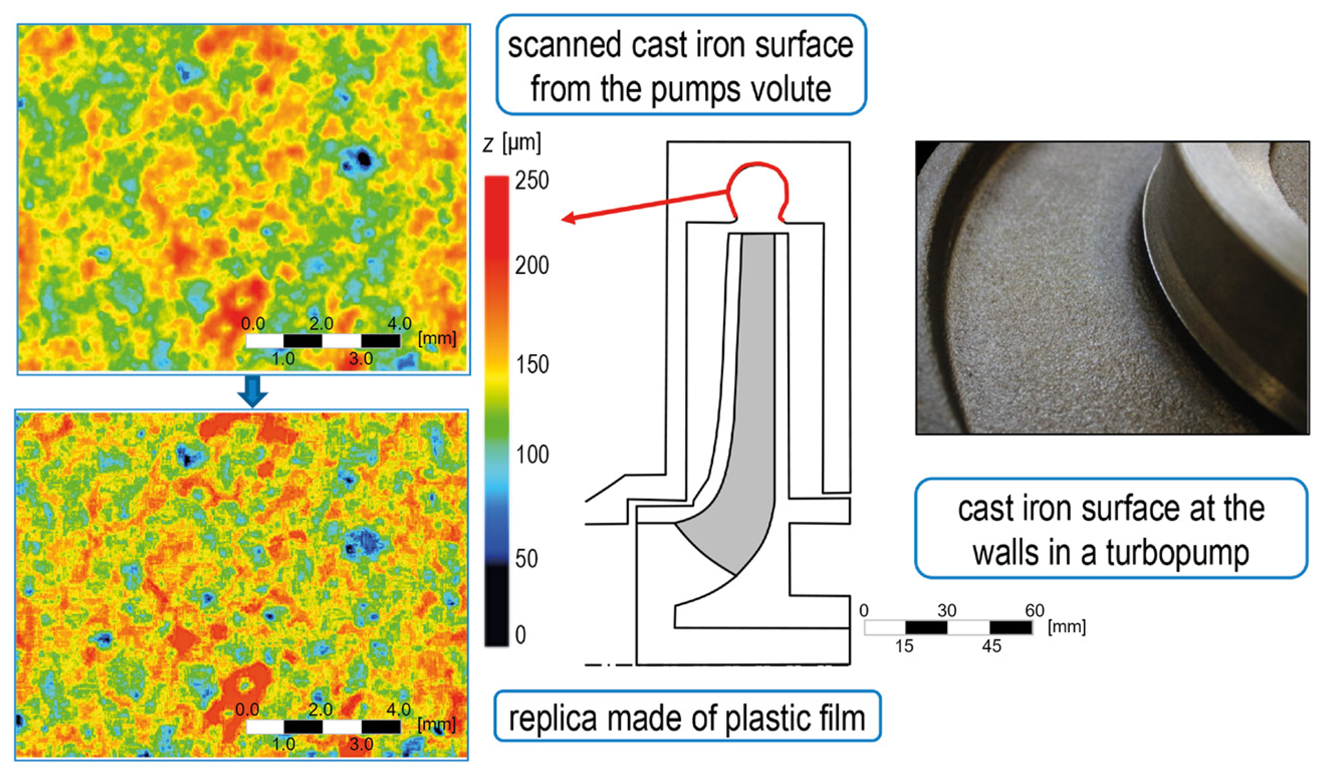
2.1. Generation of Identical and Reproducible Rough Walls for the Experiments

In order to adjust and validate the performed simulations, the flow in the channel and in the turbopump (both with rough walls) were investigated experimentally. Therefore, surface replicas of cast iron were generated artificially and attached to the smooth walls in the experimental setups.

In cooperation with the company Schweißtechnische Lehr- und Versuchsanstalt Mecklenburg–Vorpommern GmbH (Rostock, Germany), a process has been developed to similarly replicate the irregularly rough surface of cast iron. The cast iron surface at the volute of a serial, sand casted, radial turbopump was selected in this study. The surface roughness of this scan and its $k_s$ can be seen as a representative for the whole volute since the volute was made from one piece of material with one machining process (sand casting). Before the actual replication process started, the surface of the volute was optically recorded with a 3D-confocal microscope. During scanning, a spatial resolution of 1 nm in height and $1.5$ μm in transverse direction could be achieved.

A commercially available, self-adhesive plastic film with a thickness of $360$ μm served as the replica material, which was attached to the walls in the channel and turbopump experiments. The replication process was carried out by removing material from the plastic films step by step with a picosecond laser in a 5-axis machining system. The accuracy of the replication process was $10$ μm in height and $22$ μm in the flow direction and span-wise direction. The replica surface (average roughness height $k_a=20.3$ μm; maximum peak-to-trough roughness height $k_t=270$ μm) had a basic area of 12.6 mm × 9.0 mm. Since the channel walls in the experiments have a larger area than the scanned roughness area, the replica was repeated at the plastic film to fill the surface. Therefore, the basic areas were mirrored at the edges of the specific replica to avoid discontinuities at the plastic film. Figure 3 shows the height profile of the scanned cast iron surface and the replica in comparison and

Table 2. Comparison of the roughness topographical properties between the cast iron scan and the replica.

Roughness	$\overline{h}\left[\mathsf{\mu }\mathrm{m}\right]$	$k_t\left[\mathsf{\mu }\mathrm{m}\right]$	$k_a\left[\mathsf{\mu }\mathrm{m}\right]$	$k_{\mathit{rms}}\left[\mathsf{\mu }\mathrm{m}\right]$	$\mathit{Sk}$	$\mathit{ES}$
Scan	190	280	20.0	25.5	−0.12	0.24
Replica	186	270	20.3	26.1	−0.22	0.16

shows a comparison between the scanned and the replicated roughness.

For most geometrical properties between scan and replica, such as $k_a$ and $k_t$, the average roughness elevation $\overline{h}$ or the root-mean-square roughness height $k_{rms}$ are similar. Therefore, the replica has successfully imitated the original roughness in terms of height and elevation. The basic trend of negative skewness $S_k$ has remained the same indicating a pitted surface [22], which has become stronger with the replica. Additionally, for effective slope $ES$, a discrepancy has occurred, in which the replica’s value has decreased. This reduction means that the replica has become a longer wavelength roughness than the original scan. The differences in $S_k$ and $ES$ lie in the stream- and spanwise discretization of the replica, limited by the laser beam thickness. This might have an influence on the $k_s$-value between the original cast iron and the replicated surface. A discussion on this will be given in the limitations in Section 4.

2.2. Experimental Setup of the Rough Channel Flow Simulations

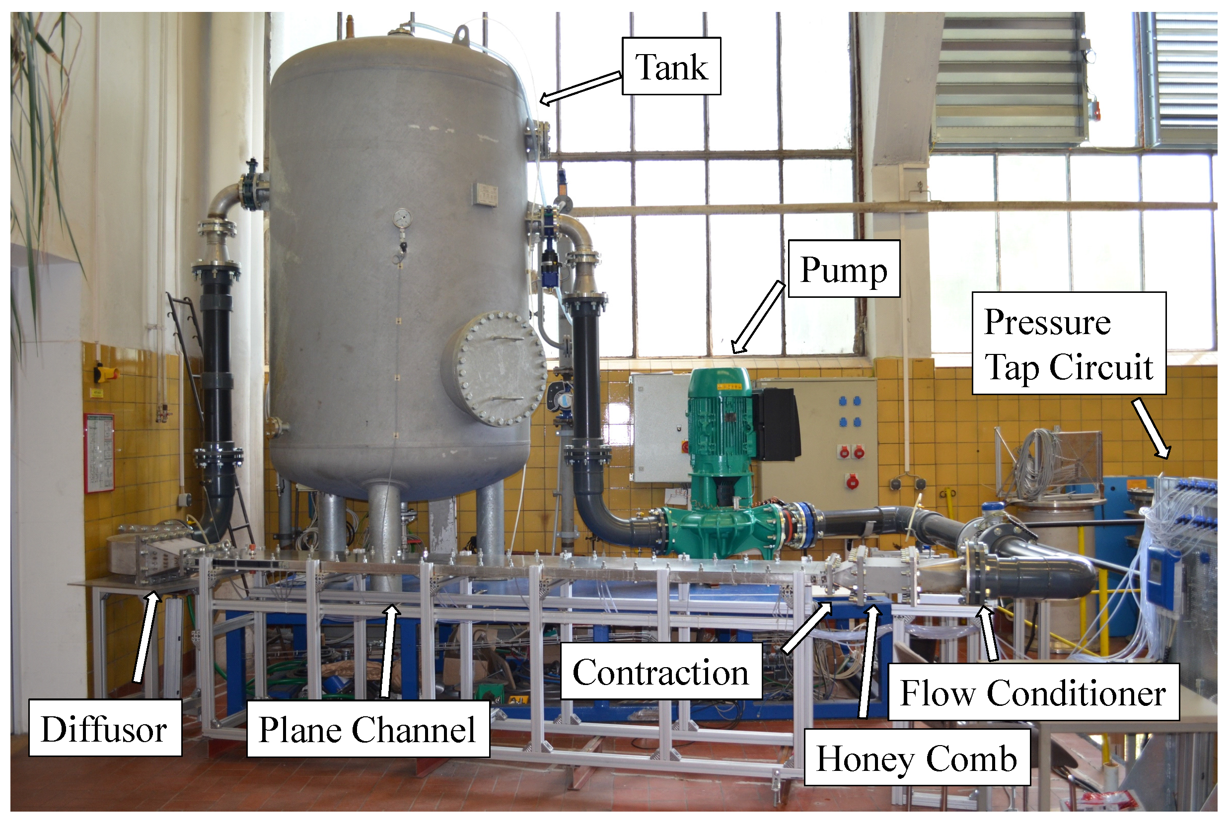
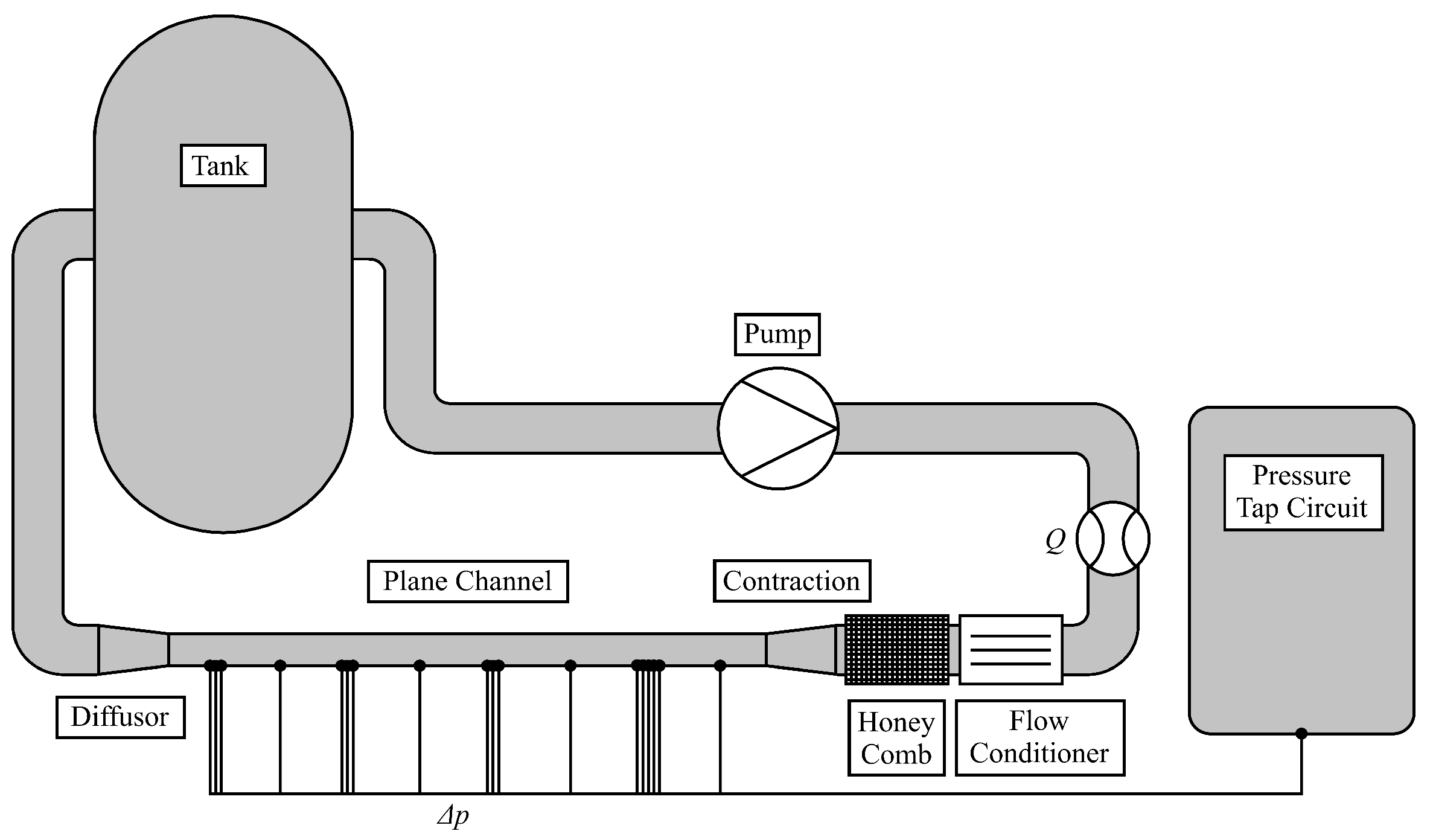
A simple flow configuration was chosen to perform the DPM simulations in order to determine $k_s$ of the rough surfaces. This simple flow configuration is a planar flow channel with rough walls in a closed-loop test rig. The test rig is shown in Figure 4 and Figure 5.

2.2.1. Test Section

The main component of the test rig is a plane channel. The channel was designed according to the work of Schultz and Flack [35] with a channel height of $H=0.025$ m and a length of $L=3$ m. The width has been determined from Jones [38] to be 12 times the channel height, resulting in a channel width of $w=0.3$ m. This width ensures an approximate plane flow at mid of the channel. Trip wires of $1.6$ mm diameter were placed at the channel entrance to provide instantly a turbulent flow. These wires create $13\%$ blockage, which is comparable to the $15\%$ blockage in Schultz and Flack [35].

An important condition for the reliable flow measurements is the precise realisation of the geometric dimensions of the channel. Due to these requirements, the channel was made of stainless steel plates, which were ground by machine. With this procedure, an average roughness height of $k_a=1.6$ μm and tolerances for flatness and parallelism of <0.2 mm and <0.1 mm were achieved, respectively.

Before entering the channel, different flow conditioners and manipulators were included, to guarantee a fully-developed channel flow. First, a 3-8-6 flow conditioner, designed with the help of DIN EN ISO 5167-2 [39], was arranged as a flow-straightener behind a pipe bow near the channel. Then, a honeycomb was placed, which contains a tube bundle of $0.006$ m diameter and $0.113$ m length, to reduce the swirl created by the pump. The tube diameter and length were determined using Ref. [35]. After the honeycomb, a contraction was placed, which was designed by a third degree polynomial [40] and connected the pipe system with the rectangular channel. After the channel, a diffuser transforms the channel geometry back to the pipe geometry. This diffuser includes a splitter to avoid flow separation in the test rig.

2.2.2. Surface Roughness

The material of the channel is ground stainless steel. Since the roughness of this material is small, a hydraulically smooth flow behaviour can be expected for the manufactured channel. To account for a channel flow with rough walls, the plastic films with the replicated cast iron surface were attached to the upper wall of the channel. Only the upper side of the channel was covered with the roughnesses so that the pressure measurements taken on the bottom side would not be distorted by the roughness. Therefore, a hydraulically smooth flow prevails at the bottom channel side, which was not considered in the evaluation of the results. The entire width of the upper channel side and ≈95% of the length were covered with the roughness.

2.2.3. Measurement System and Procedure

A flow meter was placed behind the pump to control the experimental flow rate. The pressure gradients of the channel were measured at a specific flow rate. Therefore, 17 pressure measuring holes at eight positions were included at the hydraulically smooth bottom side of the channel, see Figure 6. The pressure measuring holes have a diameter of $0.5$ mm and were eroded in the stainless steel plate to guarantee that edges of the eroded holes are burr-free and remain sharp. The holes are positioned in the centerline of the channel with a distance of (300–400) mm to each other. Furthermore, additional holes were added at measurement positions I, III, V, and VII in the traverse direction. These additional holes were 65 mm apart from the centerline holes and were used to check the flatness of the flow. The pressure gradient of the whole channel was determined by including only the pressure measurements from the centerline holes. The pressure gradient of the whole channel was obtained by averaging the pressure gradients measured in every segment between position III and VI. Therefore, a differential pressure transmitter was used, which measured the pressure difference in these segments for 2 min with a frequency of 10 Hz. This procedure was verified in a preliminary study with a smooth channel flows at different Reynolds numbers. Here, the measured pressure gradients agreed with the empirically determined pressure gradients by ≤3%.

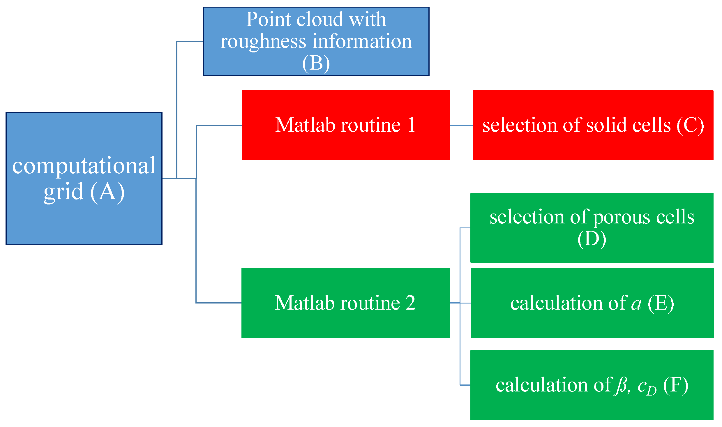
2.3. Numerical Treatment of Rough Surfaces: Discrete Porosity Method (DPM)

The discrete element method (DEM) is the basis for our method. It has already been introduced in 1985 by Taylor et al. [41] and was used by Magagnato et al. [42], Pritz et al. [43], and Stripf et al. [44] for the computation of flows at rough turbine blade walls. The DEM can be seen as an intermediate path from a discrete mapping of the surface structure in the computational domain to a complete modelling of rough surfaces. The fundamental idea of this method is the introduction of an additional sink term in the governing equations to represent the increased drag force due to the roughness effects. For the modelling, Stripf et al. [44] resort to the drag coefficients of individual basic bodies, which are determined on the basis of empirical correlations and surface measurements. Similarly, Busse and Sandham [36] have introduced a parametric forcing approach (FPA) which has been improved by Forooghi et al. [23]. It is based on the treatment of porous media using the Darcy–Forchheimer Equations.

2.3.1. Rationale of the DPM Method

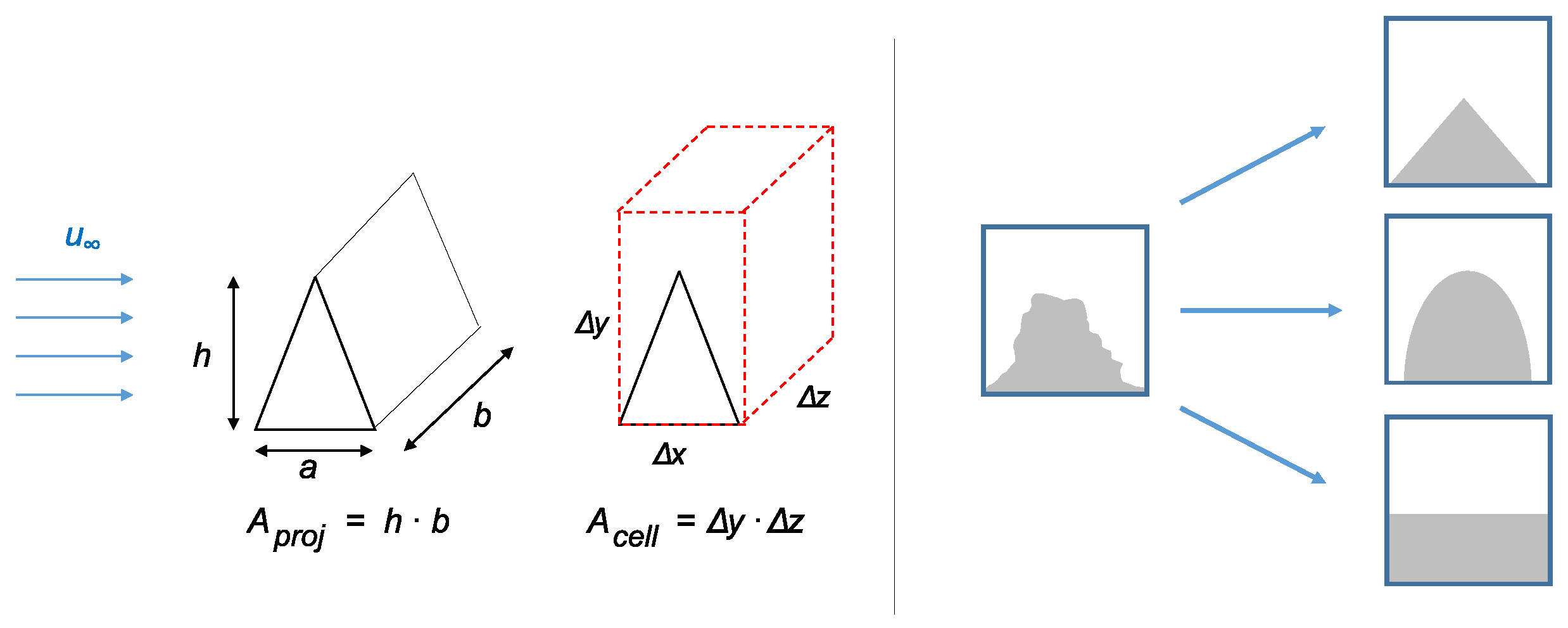
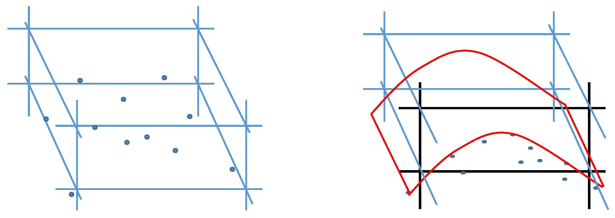
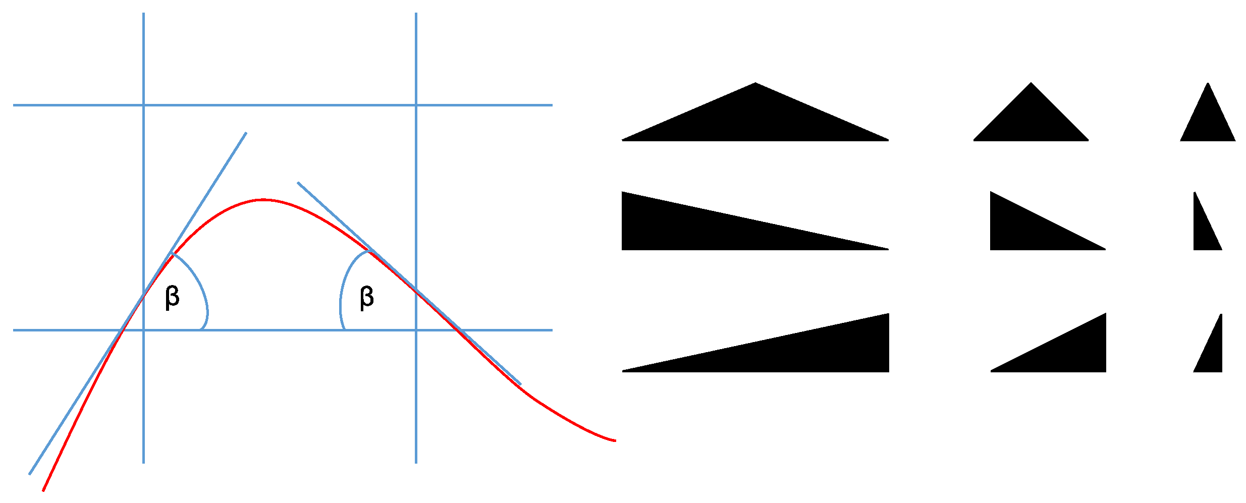
The discrete porosity method (DPM) is a self-designed simulation method for flow simulation over rough walls. The starting point represents a computational domain in which at least one wall covered with roughness elements. This domain is discretised by a computational Cartesian grid. To separate the flow from the roughness elements, three cell types are distinguished in the computational grid. Firstly, fluid cells that lie in the fluid domain and have no contact with the roughness. The governing equations, e.g., the incompressible Navier–Stokes equation (Equation (3)), are solved in these cells. Secondly, solid cells that lie completely in the roughness elements are deleted out of the mesh. Thirdly, in the Navier–Stokes equation of porous cells, that are partially filled by the roughness elements, a sink term is added on the right hand side resulting in Equation (4). The two latter cell types are also described as the roughness zone in the following. Figure 7 illustrates the described differentiation.

The authors recommend to use a plane channel flow with two wall boundary layers and periodic boundaries in the flow direction and span-wise direction for the DPM. The roughness can be placed at one wall and should be meshed separately in the roughness zone (height of this zone should be $k_t$). In this zone, the grid should be built such that a single cell resolve at least 1/5 of $k_t$ according to the authors’ experience with irregular roughnesses.

$$\frac{\partial \overrightarrow{v}}{\partial t}+(\overrightarrow{v}·\nabla )\overrightarrow{v})=-\frac{\nabla p}{\rho }+\nu \Delta \overrightarrow{v}$$

(3)

$$\frac{\partial \overrightarrow{v}}{\partial t}+(\overrightarrow{v}·\nabla )\overrightarrow{v})=-\frac{\nabla p}{\rho }+\nu \Delta \overrightarrow{v}+\frac{\overrightarrow{S}}{\rho }$$

(4)

In the porous cells, the pressure loss due to the roughness elements is calculated by an additional sink S, representing a drag (for simplicity, a roughness element with the constant width b in a flow only with the velocity component $u_{\infty }$ is assumed for the following equations). The connected drag force $F_D$ is defined by Equation (5), where $u_{\infty }$ is the flow velocity inside the cell and $A_{proj}$ is the projected area of the roughness inside the porous cell.

$$F_D=\frac{\rho }{2}{c}_D{u}_{\infty }^2{A}_{proj}$$

(5)

An example of the definition of the projected area $A_{proj}$ in Equation (5) is shown in Figure 8 for a regular roughness element. It is first assumed that the roughness fills the cell over the entire length of the porous cell $\Delta x$. To scale the influence of the roughness according to its filling of the cell, the volume fraction $\alpha$ of the roughness is introduced by Equation (6).

$$\alpha =\frac{V_{roughness}}{V_{cell}}=\frac{A_{proj}·a}{A_{cell}·\Delta x}=\frac{A_{proj}}{A_{cell}}$$

(6)

In Equation (6), a and $\Delta x$ are elided since they are assumed to be equal. If one converts Equation (6) according to the projected area and substitutes this into Equation (5), one obtains the drag force $F_D$ by:

$$F_D=\frac{\rho }{2}{c}_D{u}_{\infty }^2\alpha A_{cell}.$$

(7)

Every blunt body in a flow indicates a pressure loss $\Delta p$. As a simple relationship, Equation (7) can be normalised to the cell area. Thus, the pressure loss caused by the drag force of the roughness element in the cell can be expressed by Equation (8).

$$\Delta p=\frac{\rho }{2}{c}_D{u}_{\infty }^2\alpha$$

(8)

In order to obtain the pressure gradient in the flow direction (equal to Equation (4)), Equation (8) is normalised with the length of the cell $\Delta x$ so that Equation (9) applies for the sink S, which is added to the incompressible Navier–Stokes equation of the porous cells. The same procedure has been applied for the other directions to account for a 3D roughness element.

$$S=\frac{\Delta p}{\Delta x}=\frac{\rho }{2}{c}_D{u}_{\infty }^2\frac{\alpha }{\Delta x}$$

(9)

At this point, the analogy should be explained why the calculation of roughness effects in a flow can be described by the flow through porous media:

In any flow around a blunt body, drag force acts on the body, as well as on the flow. Because of the disturbance of the drag force in the flow, a pressure drop results out of the arising energy loss. No matter whether the body is in the free stream or on the wall, this disturbance and resulting pressure drop arises in any case. Only when the body is as small or smaller as the viscous sublayer of the wall, the disturbances may be negligible due to the dominating viscous damping of the fluid.

The flow through porous media is also affected by pressure drop, according to Darcy’s law involving viscous drag. Forchheimer added a term, representing form drag resulting in the Darcy–Forchheimer equation. The basis of the DPM is to model the pressure drop around the blunt bodies (roughness elements) with this porosity approach from Darcy–Forchheimer. This has also been performed successfully for the roughness modelling in other literature studies so far, such as in Forooghi et al. [37].

2.3.2. Determination of $\alpha$ and $c_D$

The drag coefficient $c_D$ used in Equation (9) actually refers to the flow around a regular 2D body. To describe the roughness surface with this parameter, an approximation of the real 3D roughness shape to 2D regular bodies has to be made, see Figure 8. For this geometry approximation, all roughness heights within a porous cell are selected, as exemplarily shown on the left side of Figure 9. The contained roughness heights are then two-dimensionally projected onto the black marked area on the right side of Figure 9. In the next step, the angles $\beta$ of the red contour are determined to approximate the regular shape from the real roughness distribution in the cell, see Figure 10. A set of conditions is then used to select the regular body shape according to the corresponding angles $\beta$. For example, a rectangle would be selected if both angles are between ${75}^{\circ }$ and ${90}^{\circ }$ or between $0^{\circ }$ and ${15}^{\circ }$. Otherwise, right-angled or isosceles triangles would be selected that have discrete angles of ${15}^{\circ }$ to ${75}^{\circ }$. Negative or positive sign of the angle determines, whether a left or right sided rectangular triangle is chosen for $c_D$, respectively. This procedure has been applied in the streamwise and spanwise direction. Figure 10 illustrates examples of available triangles. The approximation of the real roughness distribution to a regular body shape in a porous cell takes place in a self-written MATLAB code.

The drag coefficients $c_D$ of a large number of regular shapes and Reynolds numbers from $Re$ = 1000–200,000 were determined by additional simulations. The Reynolds numbers for these 2D RANS computations were defined by the fluid viscosity $\nu$, the free stream velocity $u_{\infty }$ at the inlet and the height h of the triangle or rectangle of regular shapes. The drag coefficients for a specific $Re$ were applied at the corresponding Reynolds number $R{e}_H$ of the channel flow simulation.

The domain size for the 2D simulations has been chosen as 40 × 40 times the height h with the regular shape placed in the center. A constant velocity and a zero pressure were given at the inlet and outlet, respectively. Furthermore, periodic boundary conditions were applied at the two other boundaries. The resulting $c_D$-values were stored in a database. This database is given in the Supplementary Material.

2.3.3. Implementation of the DPM

To realise the DPM, it was implemented in two steps. At first, the cell assignment (fluid, solid, and porous cells) was defined and the calculations of $\alpha$, $\beta$, and $c_D$ were performed in MATLAB R2019a (MathWorks Inc., Natick, MA, USA). The procedure is sketched in Figure 11. In this first step, a 3D grid (A) was created for the computational domain (explained in Section 2.4). Then, the self-written MATLAB code reads this grid, as well as a 3D point cloud (B) representing the rough surface. This point cloud was created during the scanning procedure of the pumps volute for the cast iron surface. With the given roughness height distribution from the point cloud, the roughness zone for the solid (C) and porous cells (D) was selected for the computational grid. Afterwards, the volume fractions $\alpha$ were calculated for each porous cell (E) by using the point cloud and the grid information. Then, the point-to-point slope at the cell edges defines the angles $\beta$, by which the approximate regular body shape (rectangle or triangle) was chosen for each porous cell (F). With the chosen approximate body shape, the associated drag coefficients $c_D$ were determined by using the values from the database explained above.

In a second step, the DPM was implemented in the flow solver OpenFOAM (ESI Group, Paris, FRA) for the simulations of the channel flow with rough walls. For the porous cells, the sink S in Equation (9) was implemented in OpenFOAM, based on the Darcy–Forchheimer model. Therefore, the $\alpha$ and $c_D$-values of every porous cell were stored in a fvOptions-file, which OpenFOAM accessed during the simulation to add the sink S to the momentum equations in these cells.

Here, two main differences of the present method can be summarized compared to DEM by Taylor et al. [41] and PFA by Forooghi et al. [23]: first, the solid cells of the grid are completely cut out from the Cartesian mesh. Therefore, the roughness topology can already be seen roughly without modelling, analogous to body conforming mesh. Secondly, the modelling part has been carried out in every porous cell. The determination of $c_D$ has been more detailed and complex, calculating the slope of incoming and outgoing angle of the surface roughness. A discrete value for $c_D$ depending on $Re$ will be chosen and $\alpha$ will be calculated for each porous cell, whereas Forooghi [23] has determined one $c_D$ for the total roughness zone. Taylor [41] has used an empirical formula to calculate $c_D$ depending on the Reynolds number.

2.4. Numerical Setup for the Rough Channel Flow Simulations

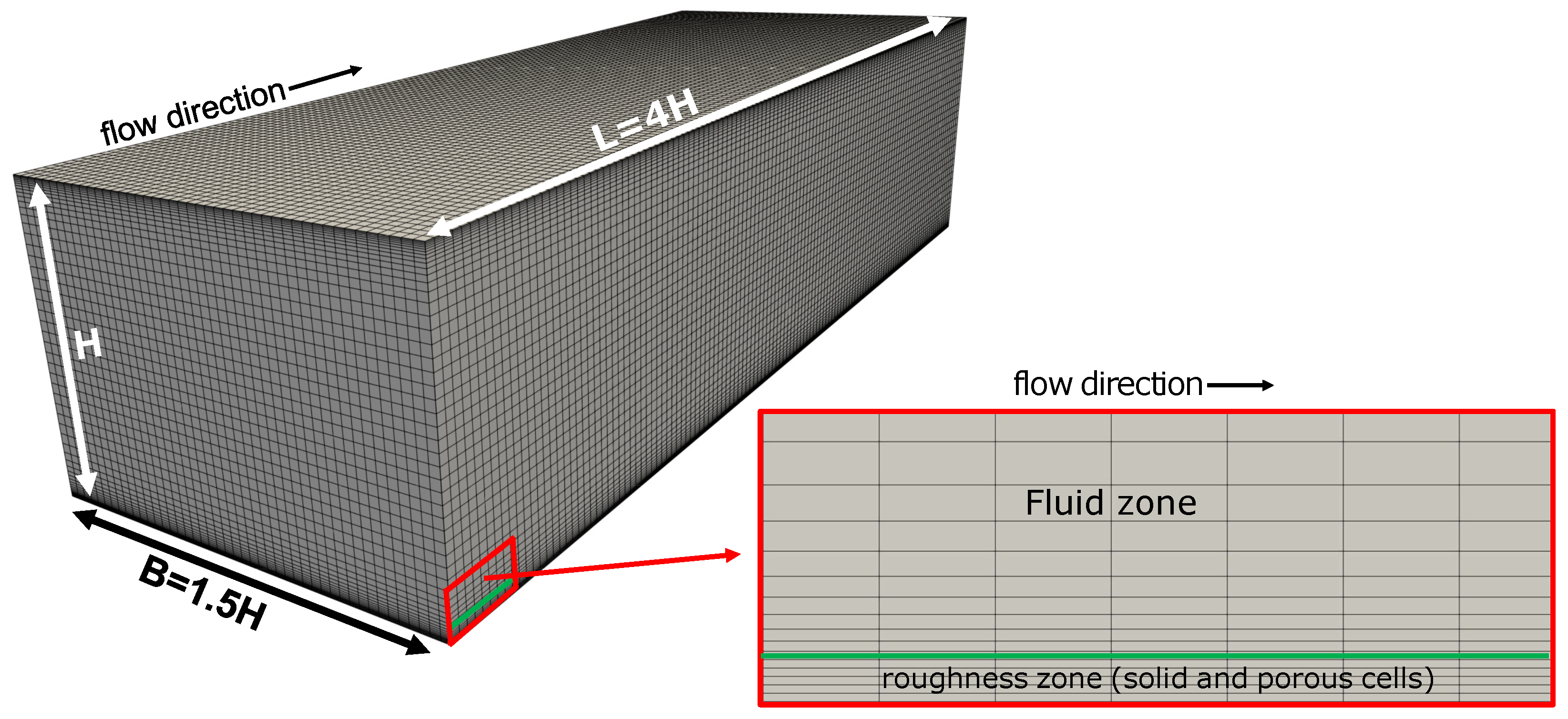
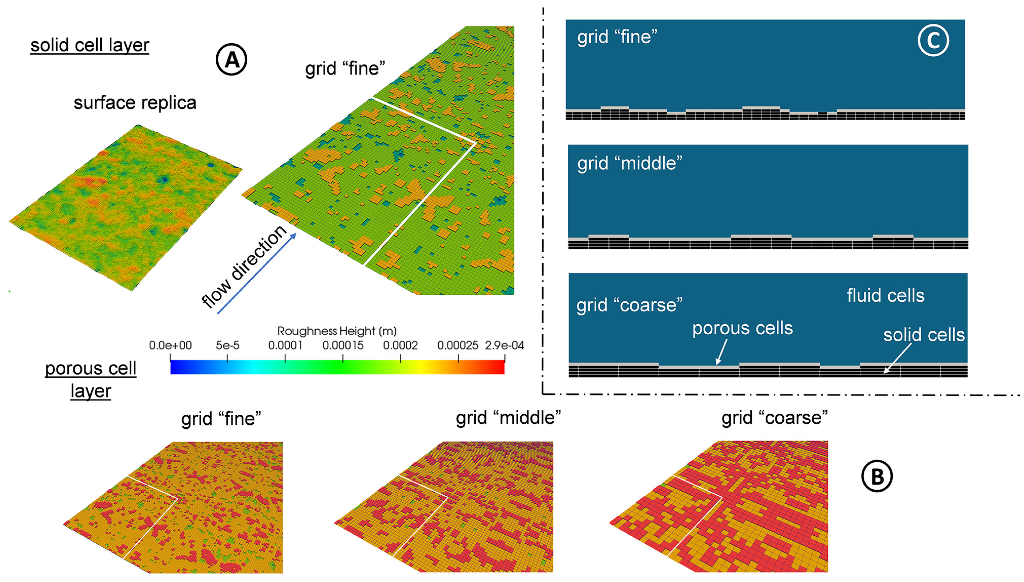
2.4.1. Computational Domain and Grid Generation

Plane channel flows with the cast iron roughness were simulated with the geometric dimensions of $(L,b,H)\approx (4H,1.5H,H)$, where H is the channel height. The channel dimensions are oriented on channel flow simulations by a study from Menter [45]. Three Cartesian, block-structured grids were created for the cast iron roughness to analyze how the DPM works on different grid resolutions, when the roughness plane $(L,b)$ is differently resolved. The properties of the four grids and an illustration of one grid are displayed in

Table 3. Properties of the three computational grids for the simulation of the cast iron roughness.

Grid Parameter	Cast Iron
	Grid ‘Coarse’	Grid ‘Middle’	Grid ‘Fine’
Grid size in M elements	0.3	1.2	4.8
Grid distribution in $(L,b,H)$	$(128,44,57)$	$(248,88,57)$	$(496,176,57)$
max. aspect ratio	13.9	7.0	4.1
max. volume change	1.2	1.2	1.2
grid angle	90${}^{\circ }$	90${}^{\circ }$	90${}^{\circ }$

and Figure 12.

The roughness zone with the solid and porous cells was defined at the bottom wall of the channel. Here, the grid was equidistantly discretised up to a height of $290$ μm in the wall-normal direction, which is the peak-to-trough roughness height $k_t$ of the cast iron surface. In this zone, the grid was built such that a single cell resolves 1/5 of $k_t$. The roughness zone of the grid ‘coarse’ is highlighted in Figure 12. The fluid zone began above the height of $290$ μm. From there, the cell height increased with a growth rate of $1.2$ compared to the cells in the roughness zone. The same growth rate was also applied in the near-wall region at the upper channel wall, where a hydraulically smooth boundary layer exists.

Since the cast iron roughness is irregularly distributed, the resolution of the roughness elements in the plane $(L,b)$ cannot be exactly defined based on the roughness geometry (as it is theoretically possible for regular roughnesses). For this reason, different grid refinements in the plane $(L,b)$ were applied.

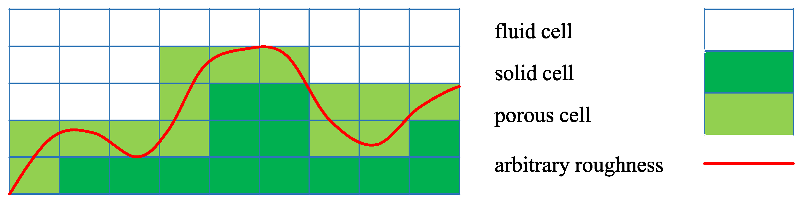
2.4.2. Consideration of the Roughness Zone (Solid and Porous Cells)

The roughness zone was defined at one channel wall, similar to the experimental setup explained in Section 2.2. A fully developed, turbulent flow is present in the channel and an URANS method was chosen to simulate the flow. After the cut-out of the solid cells, the porous cells were selected for the DPM method. Figure 13 shows the roughness zone with the solid and porous cells of the grids for the DPM simulation with the cast iron surface. Furthermore, the surface replica of the cast iron surface is illustrated in this figure.

2.4.3. Numerical Setup for the DPM Simulations

The software OpenFOAM 5.x with the pimpleFOAM solver was used to solve the governing equations by the finite volume method. The simulations were performed using URANS and the k–$\omega$–SST turbulence model [46]. Second order accurate spatial discretisation schemes were applied for the DPM simulations. The simulations were performed on the Titan high performance cluster at the University of Rostock with 144 parallel processors (Intel(R) Xeon(R) CPU E5-2640 v3 @ 2.60 GHz).

The no-slip condition applies for all walls as a boundary condition. Periodic boundary conditions were specified at the domain boundaries in the span-wise (sides) and flow direction (inlet and outlet). The flow was driven by constant mass flows $\dot{m}$ adjusted by volume forces [47] in the flow direction, which correspond to the investigated Reynolds numbers between $R{e}_H=75,000$ and $R{e}_H=400,000$ (see

Table 4. Overview of the performed DPM simulations for the channel flow simulation with the cast iron roughness.

${\mathit{Re}}_H$	Cast Iron
	Grid ‘Coarse’	Grid ‘Middle’	Grid ‘Fine’
75,000	−	✓	−
100,000	✓	✓	✓
150,000	−	✓	−
200,000	−	✓	−
250,000	✓	✓	✓
300,000	✓	✓	✓
350,000	✓	✓	✓
400,000	✓	✓	✓

). Water was used as the fluid (density $\rho =997$ kg/m${}^3$, kinematic viscosity $\nu ={10}^{-6}$ m${}^2$/s). Furthermore, turbulent boundary conditions were defined at the smooth as well as at the rough walls of the domain. Here, a zero value was specified for the modelled, turbulent kinetic energy k and the eddy viscosity ${\nu }_t$ for all simulations. A low-Re wall-function was used for the definition of the specific dissipation rate $\omega$.

The simulations were initialised by a uniform bulk velocity, a zero relative pressure and empirically determined values for the turbulent quantities in the computation domain. A time step of $\Delta t={10}^{-3}$ s was chosen. A converged flow field with a constant pressure gradient and a developed velocity profile could be observed after a time span of $T\approx 0.8$ s. Then, the simulations were continued until $T=1.1$ s. At the end of the simulations, the maximum residuals for the velocities and the pressure dropped to at least ${10}^{-3}$.

In total, 18 simulations were performed for this study, which are summarized in Table 4. Eight simulations were conducted for the cast iron surface on the grid ‘middle’ at different Reynolds numbers. In addition, 10 simulations with the grid ‘coarse’ and grid ‘fine’ were performed for Reynolds numbers $R{e}_H\ge 250,000$, where a fully rough regime was identified, and at $R{e}_H=100,000$, where experimental data were available for the channel flow with the cast iron surface.

2.5. Method for the Determination of the $k_s$-Value for the Rough Surfaces from the DPM Simulations

As a first step, the pressure gradients $\partial p/\partial x$ of the simulated channel flows were determined for every DPM simulation at a certain Reynolds number. Afterwards, the area-averaged wall shear stress ${\tau }_{w,r}$ at the rough wall had to be determined to define the non-dimensional velocity $u^{+}$ and length $y^{+}$. This wall shear stress was calculated based on a simplified momentum balance for a channel flow with a one-sided wall roughness (Equation (10)) defined by Burattini et al. [27]. The variable ${\tau }_{w,s}$ denotes the wall shear stress at the smooth channel wall in Equation (10).

$${\tau }_{w,r}=H·\partial p/\partial x-{\tau }_{w,s}$$

(10)

Subsequently, the dimensionless velocity profile $u^{+}=f\left(y^{+}\right)$ was created by the following procedure: firstly, the zero height position $y^{+}=0$ was determined by height-averaging the roughness heights and take the average value as zero height. Then, the velocities from the DPM simulations were area-averaged along the wall-normal coordinate to create a one-dimensional velocity profile $u=f\left(y\right)$. These variables were normalized to obtain $u^{+}=u/{({\tau }_{w,r}/\rho )}^{0.5}$ and $y^{+}=y·{({\tau }_{w,r}/\rho )}^{0.5}/\nu$. The characteristic downshift can be identified from this velocity profile $u^{+}=f\left(y^{+}\right)$ by comparing the simulated velocity profile with a velocity profile in the logarithmic region of the rough boundary layer based on Equation (2). This procedure was repeated for all simulations at the investigated Reynolds numbers. By plotting the roughness function $\Delta u^{+}=f\left(k_t^{+}\right)$, it was analyzed, whether a fully rough asymptote was reached, which indicated a fully rough regime [33]. Then, $k_s^{+}$ was calculated by Equation (11) [19], with $B=5.0$ and $\kappa =0.41$.

$$\Delta u^{+}=\frac{1}{\kappa }ln\left(k_s^{+}\right)+B-8.5$$

(11)

Lastly, the equivalent sand grain roughness $k_s$ was determined for the DPM simulations in this fully rough regime by Equation (12).

$$k_s=\frac{k_s^{+}·\nu }{{({\tau }_{w,r}/\rho )}^{0.5}}$$

(12)

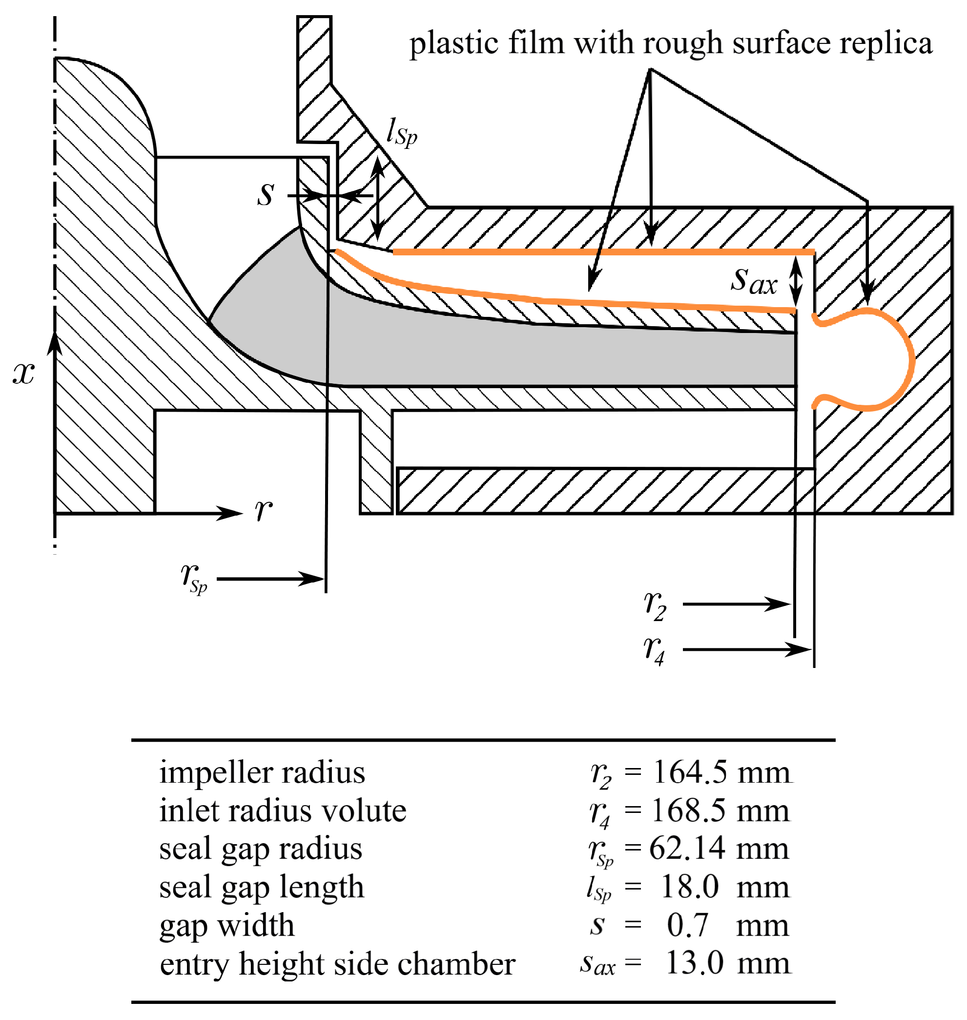
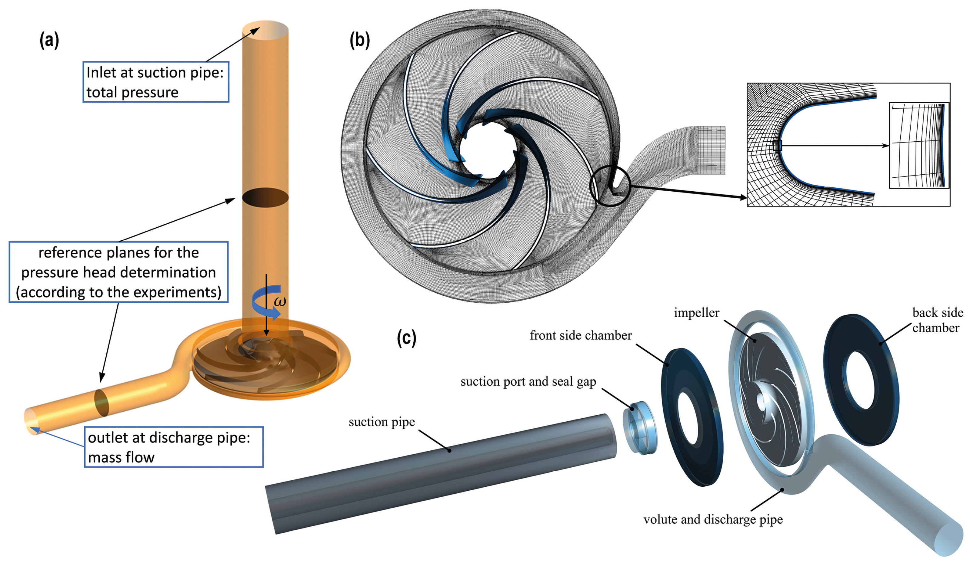
2.6. Experimental and Numerical Setup for the Turbopump Investigation

2.6.1. Numerical Setup

After the equivalent sand grain roughness $k_s$ was determined for cast iron from the DPM simulations, the $k_s$-value was specified at the rough walls in a turbopump simulation to account for the roughness effects in the pump. The investigated pump is a radial test pump with a specific speed $n_s=13.4$ 1/min. Its design was adopted from an industrial pump with minor modifications. The meridional cut through the pump, as well as the most important geometry information can be found in Figure 14. The turbopump was previously used by our institute to investigate the flow field [48] and flow losses [2,49] or the acoustics [50] in radial turbopumps with low specific speeds.

For this study, URANS computations were carried out for the turbopump using the commercial solver ANSYS CFX 2021 R1 (ANSYS Inc., Canonsburg, PE, USA). Flow governing equations were solved on a three-dimensional grid based on the finite volume method. The solver strategy was implicit with a high-resolution and an Euler backwards scheme for spatial and temporal discretization. The double precision solver executable was used. Block-structured grids with hexahedral elements were created with ICEM CFD 18 (ANSYS Inc., Canonsburg, PE, USA). All hydraulic components of the pump (impeller, volute, side chambers, sealing gap, and pipes) were considered as three-dimensional subdomains and were meshed separately. The computational domain with the locations of the inflow and outflow conditions, and some details of the computational grid are illustrated in Figure 15. An area-averaged wall distance of $y_1^{+}=1$ with a wall-normal growth rate of 1.25 was realised for all walls and all boundary layers were resolved using 26 grid cells with a growth rate of 1.25. The final grid totals $25.1$ M grid elements with a minimum grid angle of ${23}^{\circ }$. Furthermore, aspect ratios were ≤100 in $99.93\%$ of the volume. Higher aspect ratios (>100) were tolerated just in small areas ($0.01\%$ of the volume, mainly in the discharge pipe) to prevent massively more mesh elements in these areas.

The fluid properties of water at 20 °C were used (density $\rho =997$ kg/m${}^3$, kinematic viscosity $\nu$= 10${}^{-6}$ m${}^2$/s). The k-$\omega$-SST model [46] was used for closure and streamline curvature effects were accounted for with the model of Smirnov and Menter [51]. Boundary conditions were set as follows: a relative static pressure of zero value was defined at the inlet of the suction pipe together with zero gradient turbulence. Furthermore, a constant mass flow was specified at the outlet of the discharge pipe. All walls were assumed to be adiabatic and no-slip condition applies. The roughness effects were modelled in the flow solver using the approach of Lechner and Menter [8]. The sand grain roughness of $k_s=175$ μm for cast iron (determined by the DPM simulations in Section 3.2) were specified for the rough walls in the front side chamber and the volute of the pump. At these locations, the micro-structured, self-adhesive replicas with the cast iron roughness were applied at the walls in the experimental pump as well. Hence, it could be guaranteed that the same surface roughness at the same places was used in the pump both experimentally and numerically. All other surfaces in the pump were assumed to be hydraulically smooth since the manufactured pump also went through a comprehensive polishing procedure.

The performance data (pressure head, inner efficiency) of the pump were numerically determined at four operation points. Therefore, a rotational speed of $n=1450$ 1/min and flow rates of $Q=(46;65;85;93)$ m${}^3$/h were chosen to define the operation points. To couple the rotating and stationary components of the pump, the transient rotor-stator method was used with a time step equal to a ${1.5}^{\circ }$ rotation of the impeller. Convergence was reached when maximum residuals were smaller than $5·{10}^{-3}$ and all monitored values had reached a stabilised state. Each simulation was performed for 10 impeller revolutions and time-averaging for the statistical analysis of the performance data was performed over the last impeller revolution.

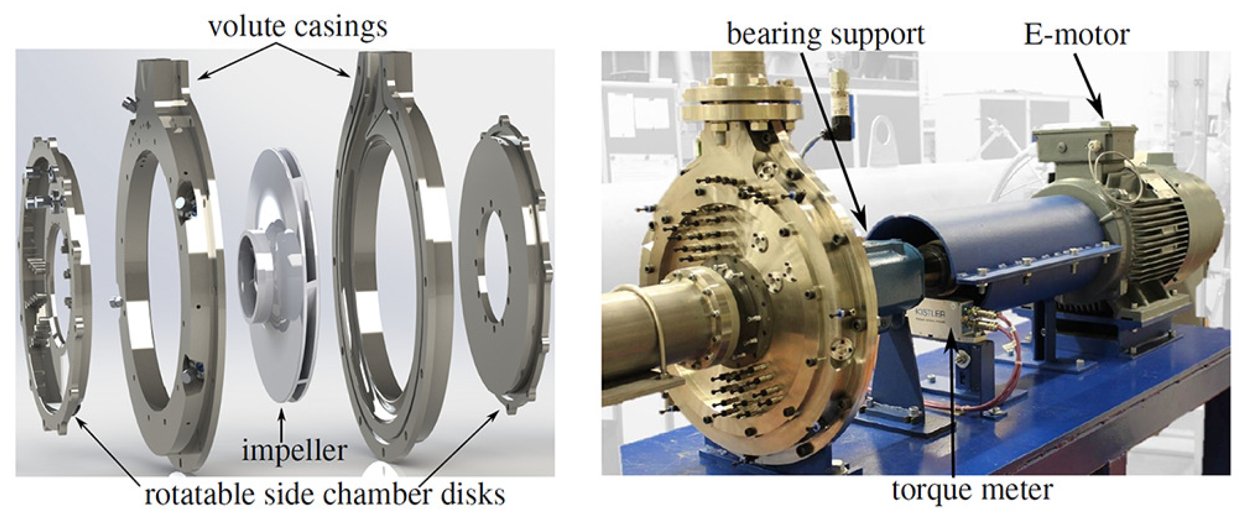
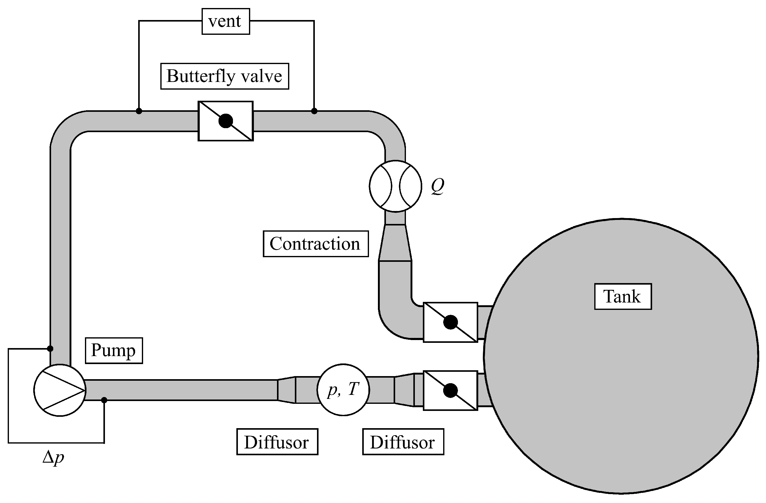
2.6.2. Experimental Setup

Experiments with the test pump (Figure 16) were conducted in order to provide a validation basis for the pump simulations with rough walls. Therefore, the original experimental pump had to be modified since all pump parts were manufactured by CNC milling with a high dimensional accuracy, and the inner surfaces were polished afterwards, so that the boundary layers indicated a hydraulically smooth behavior ($k_a\le 0.4$ μm). To account for the roughness effects of the cast iron surface, the polished surfaces of the test pump were artificially roughened with the adhesive plastic replicas containing the cast iron surface structure. Here, the wall area with replicas was limited to the whole suction side chamber and the volute, since it was shown in previous studies that the majority of the losses due to the roughness effects occur in these regions [52]. The regions where the cast iron surface replica was applied in the test pump are displayed in Figure 14.

The test pump was installed in a closed-loop test rig (Figure 17), where the (total) pressure head $H_p$ was determined by measuring the pressures at the suction and pressure side of the pump with, respectively, four pressure sensors in two ring lines according to DIN EN ISO 9906 (class 1) [53]. The flow rate was measured with a magnetic inductive flow meter, and the torque M and rotational speed n of the impeller were determined with a non-contacting measuring flange to account for the inner efficiency ${\eta }_i$ by:

$${\eta }_i=\frac{\rho ·g·H_p·Q}{M·2\pi n}.$$

(13)

3. Results and Discussion

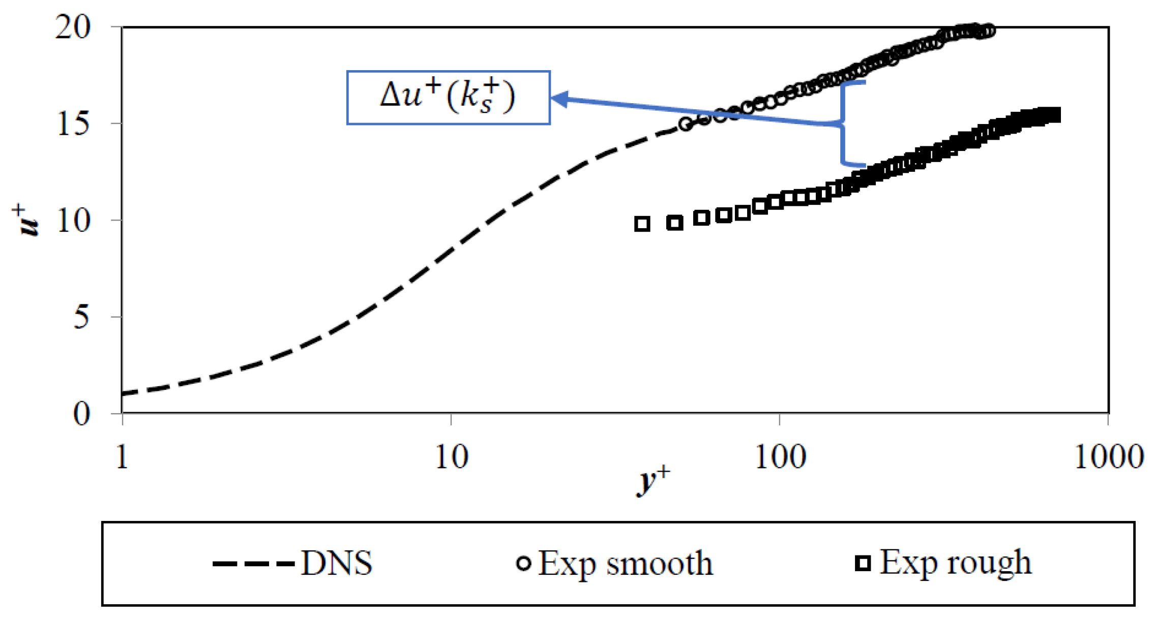
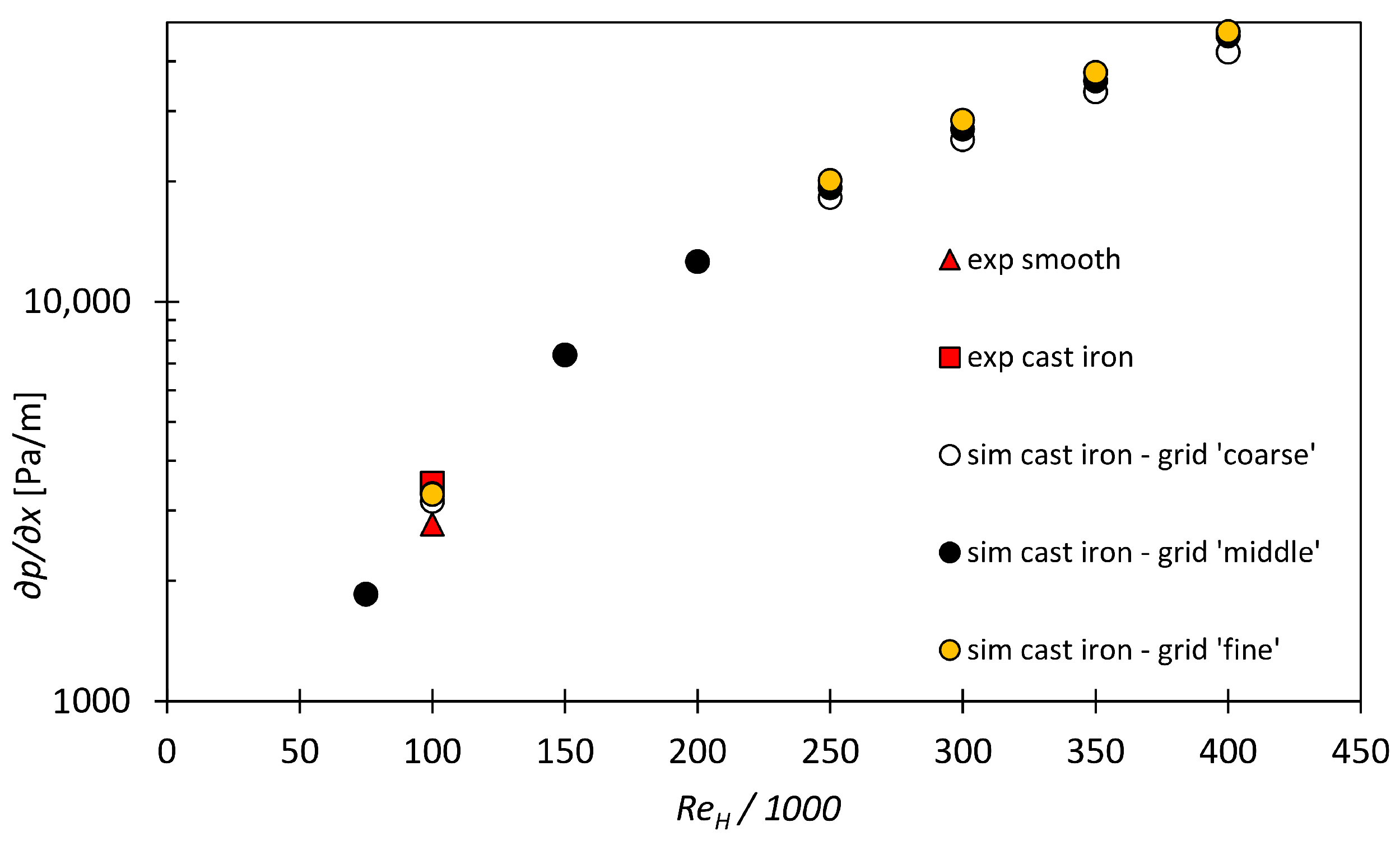
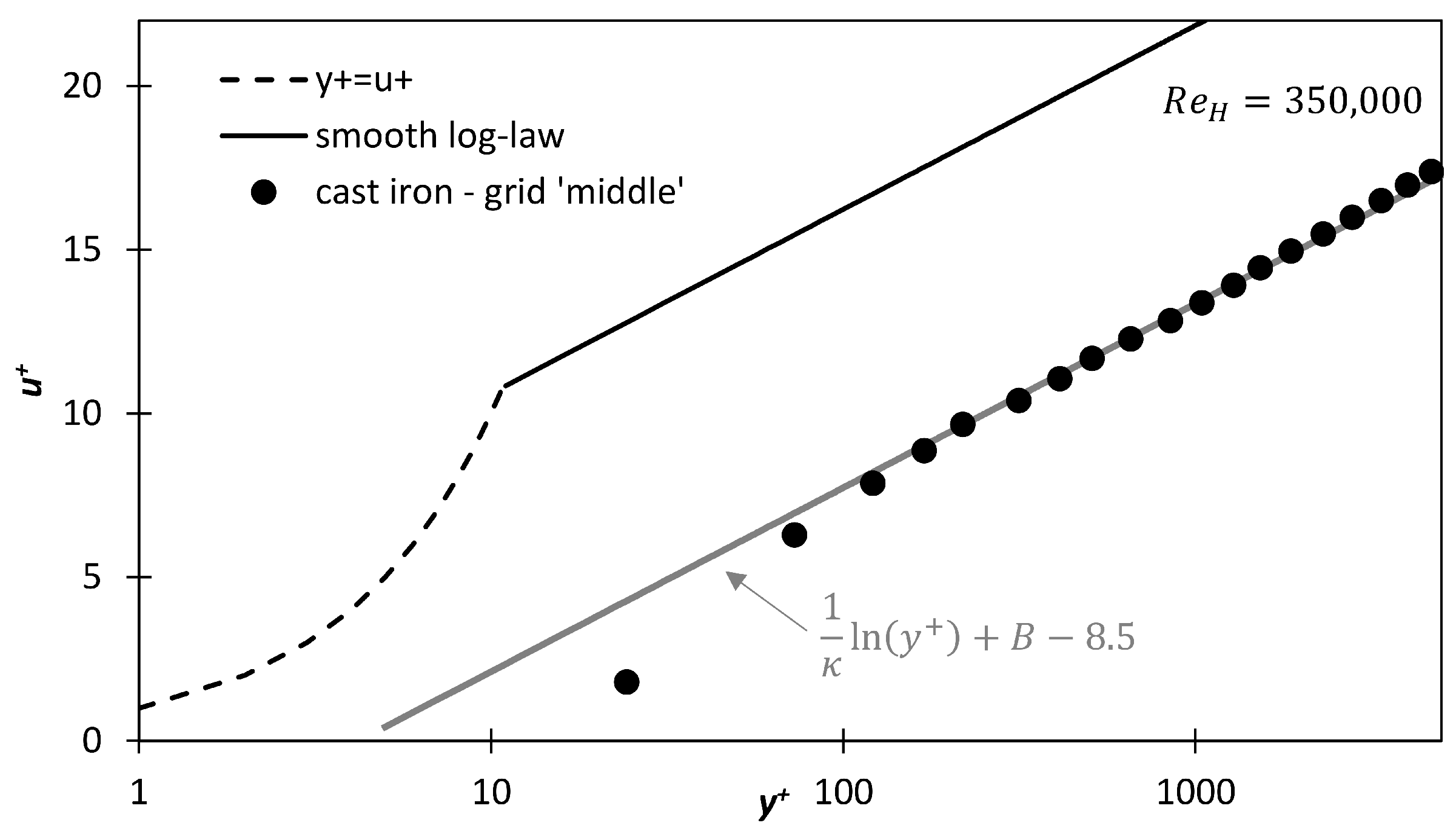
3.1. Pressure Gradients $\partial p/\partial x$ and Velocity Profiles $u^{+}=f\left(y^{+}\right)$ in the Channel Flows with Wall Roughness

The experimentally and numerically assessed pressure gradients are plotted in Figure 18. A relative deviation of ≈5% is achieved between the measured and simulated pressure gradient in the rough channel for the grid ‘middle’ and ‘fine’ at $R{e}_H=100,000$. The simulation with the grid ‘coarse’ had a higher deviation of ≈10% to the measured $\partial p/\partial x$.

In the range of $Re\ge 250,000$, where the fully rough regime is present for cast iron (explained in the next sections), the results of grid ‘middle’ and ‘fine’ also show similar pressure gradients. The grid ‘coarse’ calculates slightly lower pressure gradients at these high Reynolds numbers. At $R{e}_H=400,000$, the grid ‘coarse’ and grid ‘fine’ deviate by ≈10%, whilst the relative difference between grid ’middle’ and grid ‘fine’ is just $2\%$.

Due to the similar results of the grids ‘medium’ and ‘fine’ to each other, as well as due to the good agreement with the experimental data, the simulations on the grid ‘medium’ are used for the following evaluation and the calculation of the $k_s$-value.

Based on the pressure gradients and the procedure described in Section 2.5, the non-dimensional velocity profiles $u^{+}=f\left(y^{+}\right)$ were achieved for the DPM simulations. One exemplary velocity plot for the grid ‘middle’ at $R{e}_H=350,000$ is shown in Figure 19. The shown velocity profile was achieved at a high Reynolds numbers, where a fully rough regime is present. A significant downshift in the simulated profile compared to the log-law in the smooth boundary layer can be seen in this figure. Furthermore, there is a clear correspondence between the logarithmic velocity profile in the roughness regime according to Equation (2) and the simulated ones. This agreement was searched for each DPM simulation to calculate the roughness functions $\Delta u^{+}=f(k_s^{+},k_t^{+})$, which will be discussed in the next section.

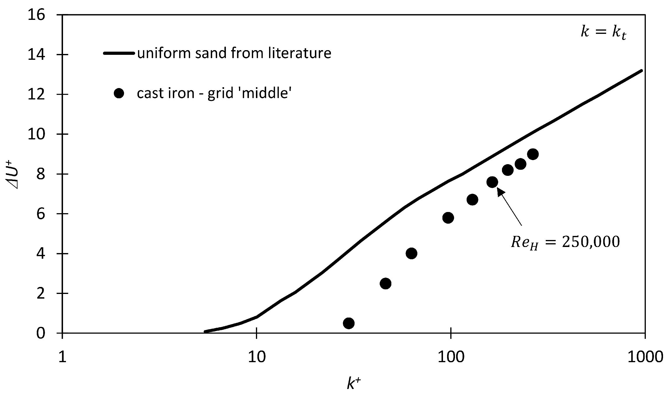
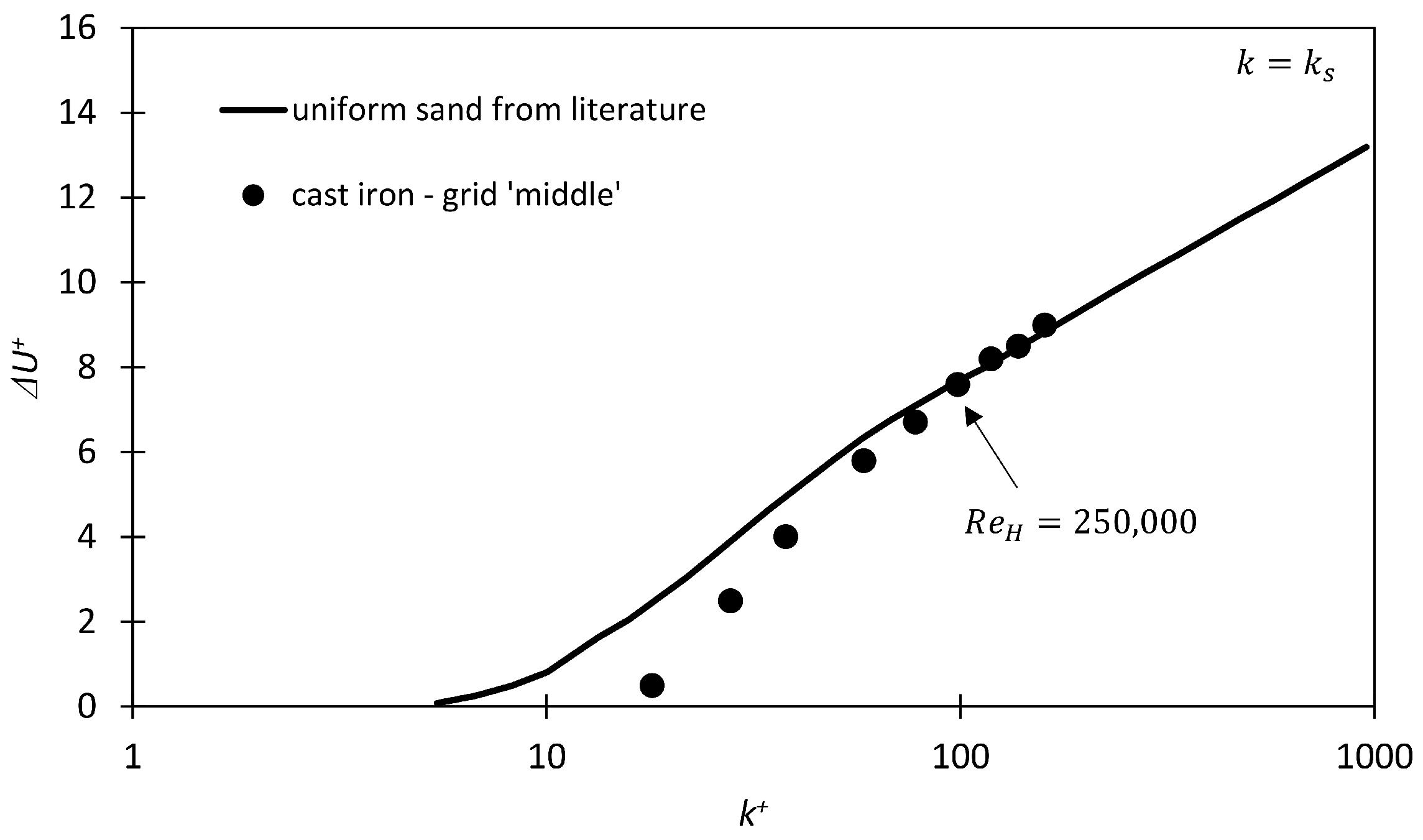
3.2. Determination of the Equivalent Sand Grain Roughness $k_s$ in the Fully Rough Regime

The roughness function $\Delta u^{+}=f\left(k_t^{+}\right)$ is plotted in Figure 20 to identify the fully rough regime, in which the appropriate $k_s$-value for cast iron can be identified. Additionally, the roughness function for uniform sand from Nikuradse [54] is included in this plot. As can be seen from this figure, an emerging asymptotic behaviour is observable for cast iron above a Reynolds number of $R{e}_H=250,000$, indicating the fully rough regime at the higher $Re$.

In these fully rough regimes, the $k_s$-value can be determined by Equation (11) and Equation (12).

Table 5. Calculated $k_s$-values for the DPM simulation with the cast iron surface at the high Reynolds numbers.

Re	Cast Iron
	Grid ‘Middle’
250,000	$k_s=168$ μm
300,000	$k_s=179$ μm
350,000	$k_s=174$ μm
400,000	$k_s=184$ μm
average	$k_s=(176\pm 8)$ μm

summarizes the $k_s$-values for the simulations at the highest Reynolds numbers. Similar values for $k_s$, with deviations smaller than $5\%$ to the mean value, are achieved for the Reynolds numbers, in which a fully rough regime is present. The sand grain roughness results in a mean value of $\approx 175$ μm. Compared to the wide ranges of sand roughness values for a cast iron surface from the literature (Table 1 on page Table 1), the $k_s$-values determined in this study are near the lower limits for $k_s$ of cast iron reported from experimental studies in Refs. [3,13,14,15,17].

After the $k_s$-value was determined, it was also checked, if the roughness functions $\Delta u^{+}=f\left(k_s^{+}\right)$ collapses with the function of uniform sand from Nikuradse [54]. This is illustrated in Figure 21. An excellent match of the roughness function is recognisable in the fully rough regime. This shows that the determined $k_s$-values of cast iron will indicate the same roughness effect in the flow as uniform sand of same height. This is necessary for the application of the $k_s$-value for roughness modelling in the following turbopump simulation, and demonstrates that the methodology for $k_s$-determination with the DPM indicate reasonable results.

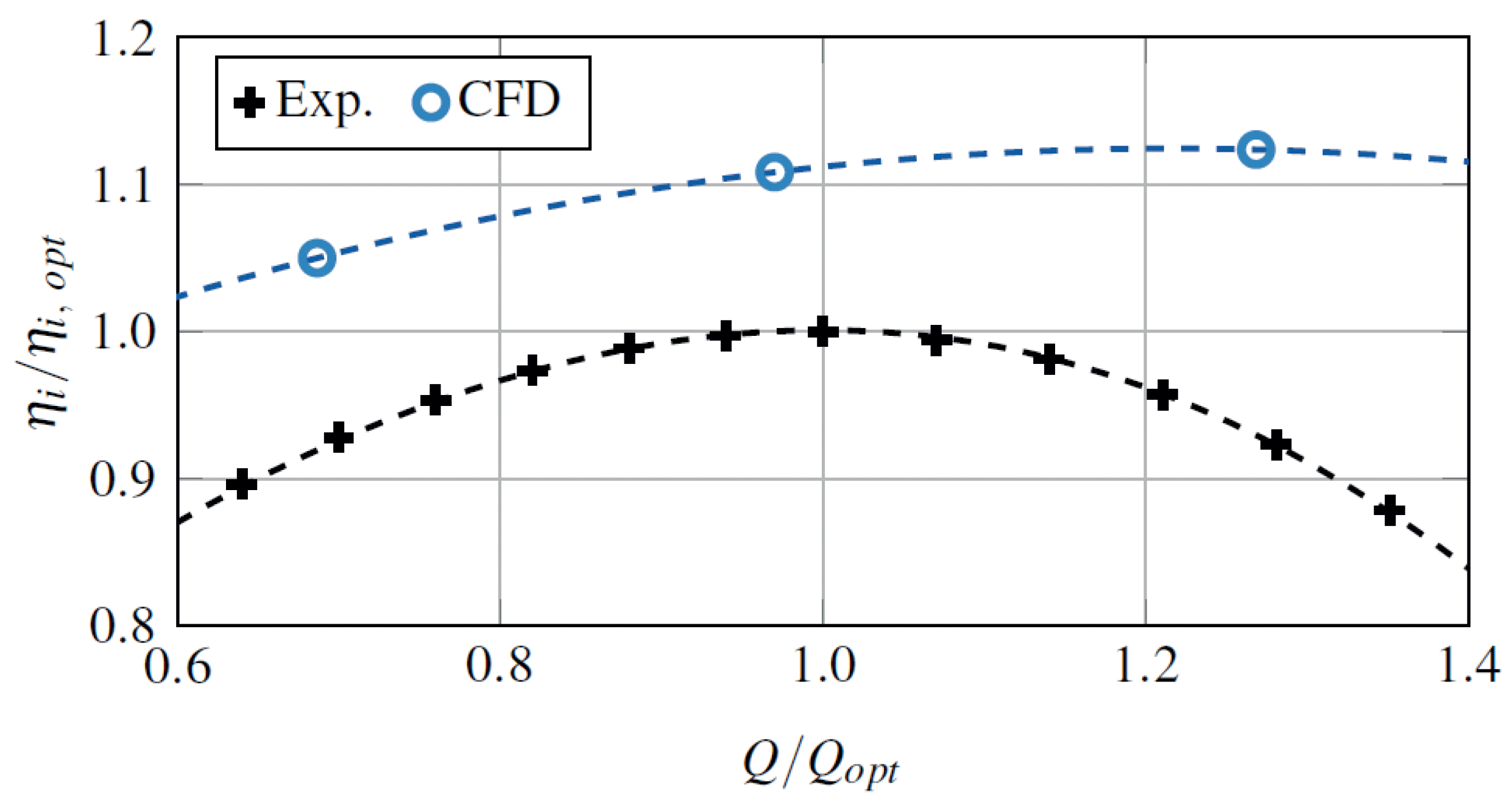
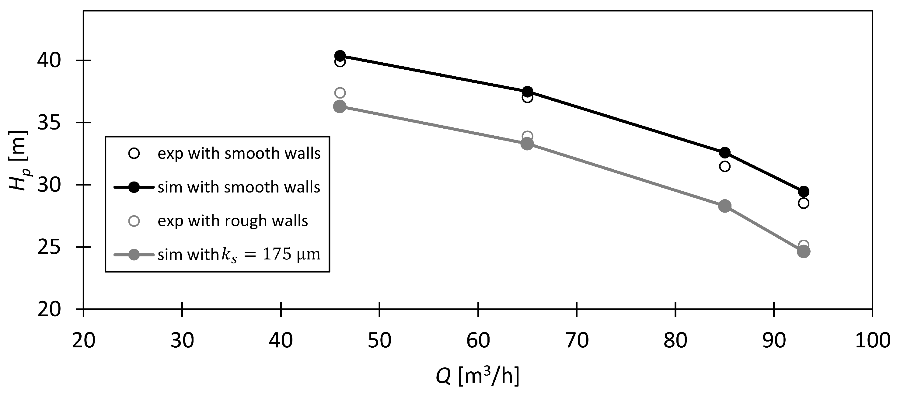
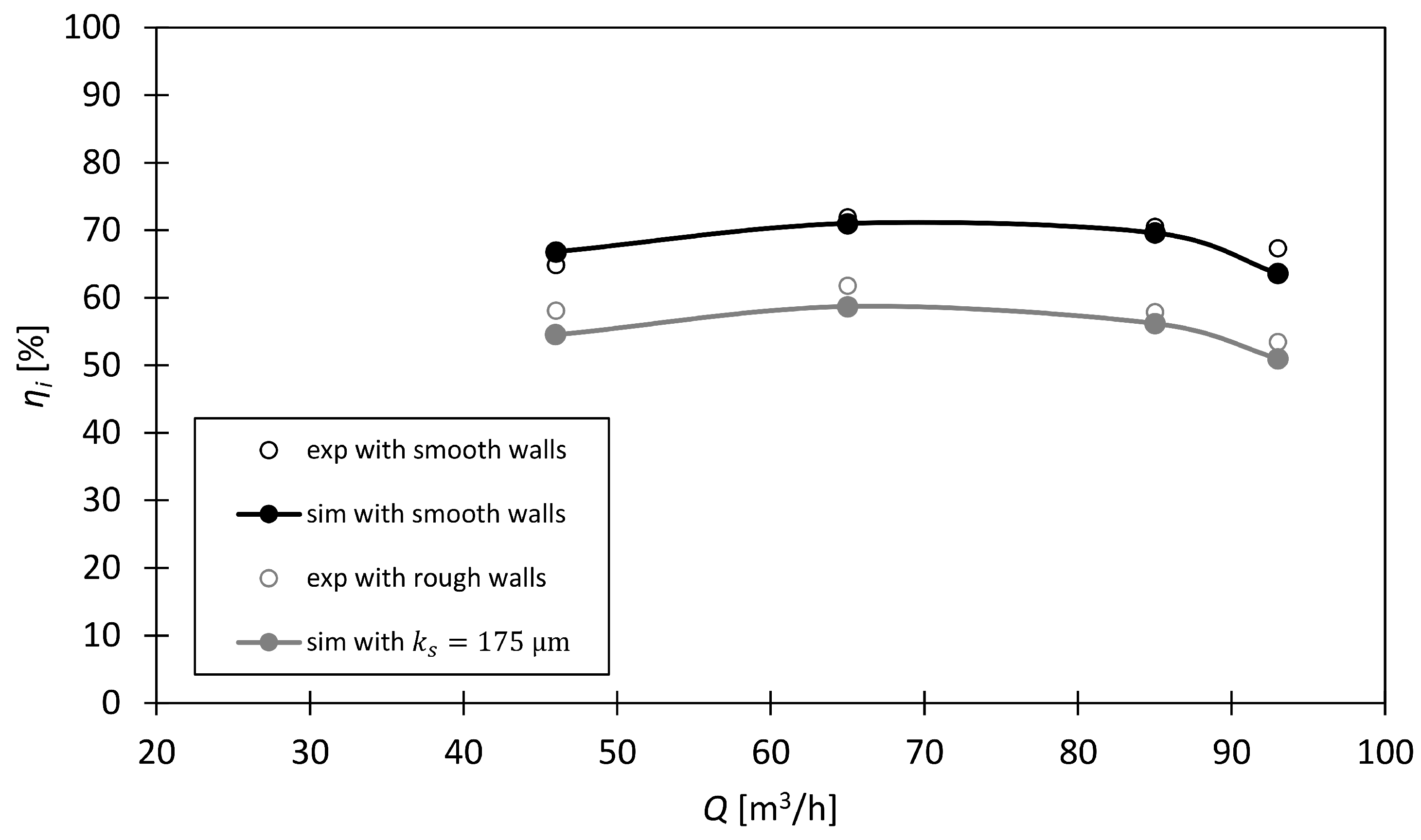
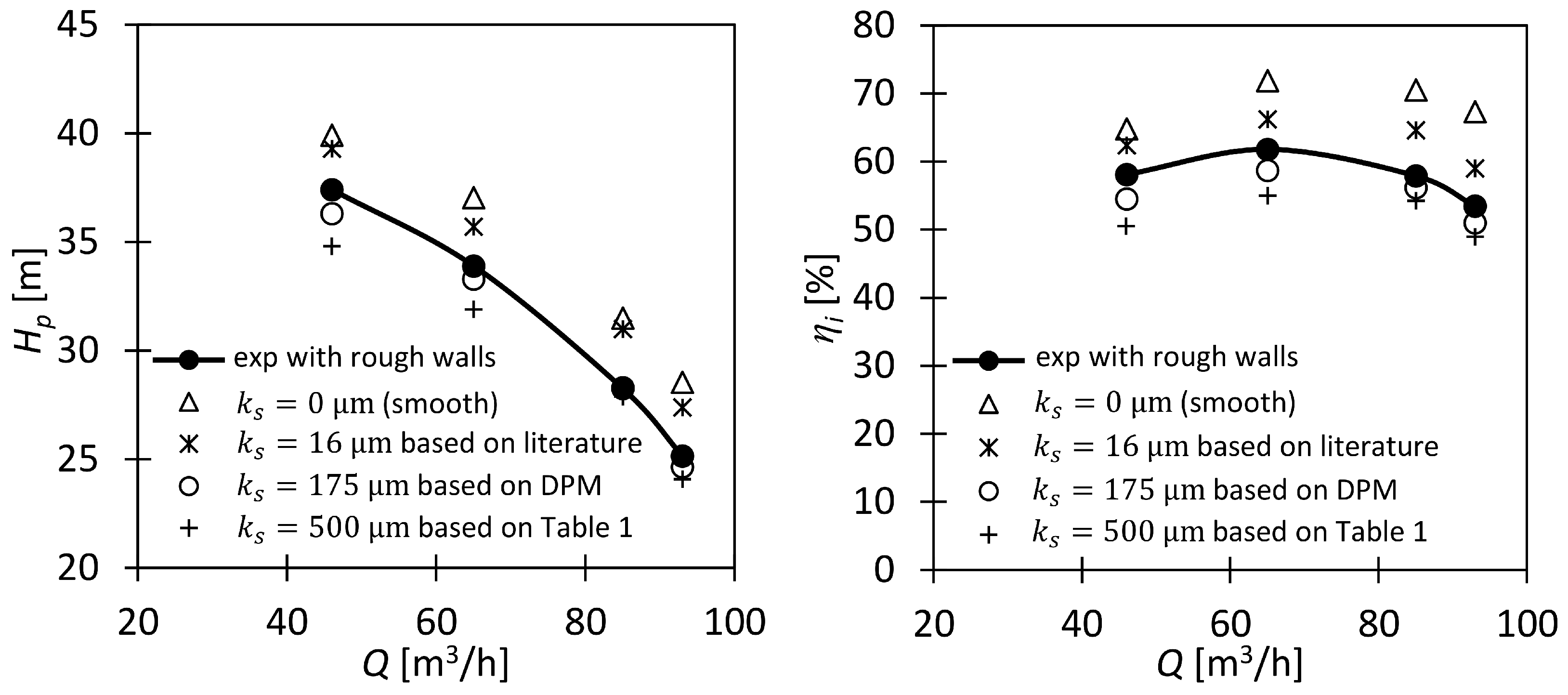
3.3. Simulation of the Performance Data in a Radial Turbopump with Wall Roughness

The simulated pressure head $H_p=f\left(Q\right)$ and efficiency ${\eta }_i=f\left(Q\right)$ curves are displayed and compared with the experimentally observed performance data in Figure 22 and Figure 23. Additionally, the simulated and measured performance data curves are displayed for a turbopump with hydraulically smooth walls. There is a good agreement in the performance data between the simulation results with the implemented $k_s$-value and the measurements of the pump with rough surfaces. The absolute deviations between experiments and numerics ranges from (0.1–1.1) m for the pressure head $H_p$ and (1.7–3.6)% for the efficiency ${\eta }_i$ along the whole performance curves. These deviations to the experimental values can be much larger if $k_s$ is estimated using empirical correlations or other literature values, e.g., from Table 1. A comparison of pump characteristics with three differently estimated $k_s$-values for cast iron is given in Figure 24.

In addition, a comparison can be made between the turbopump with rough and hydraulically smooth walls. Figure 22 shows a permanent pressure head reduction in $\Delta H_p\approx -4$ m from the ‘smooth wall’ to the ‘rough wall’ simulation case. The impact on pump efficiency is even greater if the roughness effects are not taken into account in the simulations. A constant, absolute offset of about $\Delta {\eta }_i\approx -10\%$ is present between the simulations with and without roughness consideration. These results show the importance of considering roughness effects in simulations of turbopumps with low specific speeds. The current hydraulic components (impeller, side chambers, volute) of a pump are made of cast iron or investment iron, which can exhibit significant roughness heights, especially with increasing operating time of the pump. As already shown in Figure 1 or Figure 23, significant discrepancies could exist between the experiments in a manufactured pump and the flow simulations of a computer-designed pump, when these roughnesses are unconsidered in the simulations.

4. Limitations

Although the use of DPM shows promising results, the method is still at an early stage of development. Regarding this, the DPM tries to approximate the drag in the 3D flow by calculating 2D drag values of regular body shapes. The assumption of using 2D values is made since the 3D roughness structure (in the porous cell layer of one cell height) is projected on the streamwise and spanwise cell face, to create 2D shapes in the streamwise and spanwise direction, respectively. This results in different drag values for the different directions, which are used to estimate the pressure drop in the 3D flow over a cell. The next step in extending the method will be to find an optimized way to model the pressure sink for each idealised regular body shape in the porous cells. This could be performed, for example, on the basis of an AI optimisation, where each idealised body shape in the cell is assigned a corresponding AI-optimised drag coefficient $c_d$. Additionally, there will be an influence of adjacent roughness elements on the $c_D$-value, which is currently not in the DPM formulation. One of the next steps will be to integrate this influence. All these points show that there is still room for improvement of the DPM. Nonetheless, the determination of $k_s$ works well despite the simplifications and assumptions: the rough channel flow simulation gives comparable value to the experiment (Figure 18), the $k_s$-value is in the range of the literature (Table 1 and Table 5) and the pump characteristics from the simulations agree well with the experiments (Figure 22 and Figure 23).

When comparing the original cast iron scan with the replica (Table 2), it was found that important geometric parameters, such as $k_t$ and $k_a$, were similar between the two surfaces. However, the surface parameters $S_k$ and $ES$ differed between the surfaces, which can be attributed to the manufacturing process of the replica. It does not affect the initial objective of this paper that the $k_s$-value can be reasonably determined for an arbitrary surface roughness by the DPM, since all experimental and numerical results refer to the replica. However, due to the different surface parameters, the drag in the rough boundary layer between scan and replica could be affected, which can also influence $k_s$. Regarding this, the original cast iron surface could have a higher sand grain roughness than the replica due to the larger skewness and effective slope [22]. For future studies, we will try to further optimize the manufacturing process to bring the surface parameters between scan and replica closer together.

Furthermore, the DPM channel flow simulation was just validated at one Reynolds number ($R{e}_H=100,000)$. Unfortunately, it was not possible to validate the cast iron roughness for higher $Re$ as well. The reason is that the test rig pump cannot overcome the high losses at higher Re. Currently, the test rig is modified so that roughness evaluations can be carried out at higher Reynolds numbers in the future.

5. Conclusions

The present study demonstrates a novel and time-efficient simulative approach on how to determine the equivalent sand roughness $k_s$ for irregularly distributed surface roughnesses. The $k_s$-values can then be used in the roughness modelling of complex flow simulations, e.g., in turbomachines, to properly account for the performance data.

By means of the self-designed discrete porosity method (DPM), it is possible to compute the effect due to the roughess in a simulation without directly resolving the complete roughness topology. This is achieved by separating a computational grid in three zones and treating the governing equations in every zone differently. Firstly, there are solid cells, which are completely submerged by the rough surface. Therefore, the flow is completely cut out from the grid. Secondly, there are fluid cells, in which the governing equations are being solved. Thirdly, porous cells exist, which are partly covered by the roughness elements and the fluid. The roughness elements in these porous cells were modelled by idealised body shapes, which cause a drag resistance and hence, a pressure sink in the flow.

Channel flow simulations with an irregularly distributed cast iron surface were computed by the DPM at different Reynolds numbers. The velocity profiles from the DPM simulations indicated a downshift of the curves, which increases with higher Reynolds numbers and, thus, rising roughness effects. By using this downshift, the roughness function $\Delta u^{+}=f\left(k_t^{+}\right)$ was plotted to identify the fully rough regime, where the $k_s$-value of the roughness under investigation can be determined. For cast iron, a $k_s$-value of $175$ μm was determined, which is in accordance with literature data for cast iron. The results of the pump simulations performed with the equivalent sand roughness of cast iron showed good agreement with the experimental measurements.

In summary, the DPM represents a promising method to determine $k_s$-values of rough surfaces. The computation times of the method are low compared to a direct resolution of the roughnesses by a flow simulation. Additionally, the DPM provides just one $k_s$-value for a specific scanned surface, e.g., for cast iron, whereas the literature state a wide range of $k_s$-values for a set of cast iron surfaces. Both points will allow turbopump designers to more accurately consider rough surfaces in their design simulations in the future.

In follow-up work, the DPM will be used to determine $k_s$ for different cast iron surfaces in different parts of the turbopump, such as in the impeller or the side chambers. This will be used to investigate the influence of the zonal roughness (and its different surface topologies) on the pump performance. Additionally of interest to the authors is a deeper understanding of the flow in the rough side chambers of a radial pump with small $n_s$. The flow in the side chambers shows a strong interaction with the adjacent pump parts [2] and is crucial for the pump performance and the acting flow forces in the pump.

References

1. Viet, D.D.; Kumar, J.; Wurm, F.H. Modelling of wall roughness in flow simulations. In Proceedings of the 4th International Rotating Equipment Conference, Wiesbaden, Germany, 23–24 September 2019; Paper No. 071. pp. 1–11. [Google Scholar]
2. Juckelandt, K.; Bleeck, S.; Wurm, F.H. Analysis of Losses in Centrifugal Pumps with Low Specific Speed with Smooth and Rough Walls. In Proceedings of the 11th European Conference on Turbomachinery, Madrid, Spain, 23–26 March 2015; Martelli, F., Díaz, R.V., Eds.; 2015; pp. 1–10. [Google Scholar]
3. Schlichting, H.; Gersten, K. Boundary-Layer Theory, 9th ed.; Springer: Berlin/Heidelberg, Germany, 2017. [Google Scholar]
4. Schlichting, H. Experimentelle Untersuchungen zum Rauhigkeitsproblem. Ing.-Arch. 1936, 7, 1–34. [Google Scholar] [CrossRef]
5. Rotta, J.C. Das in Wandnähe gültige Geschwindigkeitsgesetz turbulenter Strömungen. Ing.-Arch. 1950, 18, 277–280. [Google Scholar] [CrossRef]
6. Flack, K.A.; Schultz, M.P.; Shapiro, T.A. Experimental support for Townsend’s Reynolds number similarity hypothesis on rough walls. Phys. Fluids 2005, 17, 35102. [Google Scholar] [CrossRef]
7. Flack, K.A.; Schultz, M.P. Review of Hydraulic Roughness Scales in the Fully Rough Regime. J. Fluids Eng. 2010, 132, 41203. [Google Scholar] [CrossRef]
8. Lechner, R.; Menter, F.R. Development of a Rough Wall Boundary Condition for Omega-Based Turbulence Models: TR-04-04, Rough Walls 1.1; ANSYS CFX: Otterfing, Germany, 2004. [Google Scholar]
9. Apsley, D. CFD Calculation of Turbulent Flow with Arbitrary Wall Roughness. Flow Turbul. Combust. 2007, 78, 153–175. [Google Scholar] [CrossRef]
10. Aupoix, B. Wall Roughness Modelling with k-w SST Model. In Proceedings of the 10th International ERCOFTAC Symposium on Engineering Turbulence Modelling and Measurements, Marbella, Spain, 17–19 September 2014; Springer: Berlin/Heidelberg, Germany, 2014. [Google Scholar]
11. Wilcox, D.C. Formulation of the k-omega Turbulence Model Revisited. AIAA J. 2008, 46, 2823–2838. [Google Scholar] [CrossRef]
12. Knopp, T.; Eisfeld, B.; Calvo, J.B. A new extension for k– turbulence models to account for wall roughness. Int. J. Heat Fluid Flow 2009, 30, 54–65. [Google Scholar] [CrossRef]
13. Wagner, W. Strömung und Druckverlust, 6th ed.; Vogel: Würzburg, Germany, 2008. [Google Scholar]
14. Fried, E.; Idelcik, I.E. Flow Resistance: A Design Guide for Engineers, first ed.; Taylor & Francis: Philadelphia, PA, USA, 1997. [Google Scholar]
15. Oertel jr., H.; Böhle, M.; Dohrmann, U. Strömungsmechanik: Grundlagen–Grundgleichungen–Lösungsmethoden—Softwarebeispiele, 5th ed.; Vieweg+Teubner: Wiesbaden, Germany, 2009. [Google Scholar]
16. Gülich, J.F. Centrifugal Pumps, 3rd ed.; Springer: Berlin/Heidelberg, Germany, 2014. [Google Scholar]
17. White, F.M. Fluid Mechanics, 4th ed.; McGraw-Hill: Boston, MA, USA, 1998. [Google Scholar]
18. Bons, J.P. A Review of Surface Roughness Effects in Gas Turbines. J. Turbomach. 2010, 132, 021004. [Google Scholar] [CrossRef]
19. Schultz, M.P.; Flack, K.A. Turbulent boundary layers on a systematically varied rough wall. Phys. Fluids 2009, 21, 015104. [Google Scholar] [CrossRef]
20. Sigal, A.; Danberg, J.E. New correlation of roughness density effect on the turbulent boundary layer. AIAA J. 1990, 28, 554–556. [Google Scholar] [CrossRef]
21. van Rij, J.A.; Belnap, B.J.; Ligrani, P.M. Analysis and Experiments on Three-Dimensional, Irregular Surface Roughness. J. Fluids Eng. 2002, 124, 671. [Google Scholar] [CrossRef]
22. Chung, D.; Hutchins, N.; Schulz, M.P.; Flack, K.A. Predicting the Drag of Rough Surfaces. Annu. Rev. Fluid Mech. 2021, 53, 439–471. [Google Scholar] [CrossRef]
23. Forooghi, P.; Stroh, A.; Magagnato, F.; Jakirlic, S.; Frohnapfel, B. Toward a universal roughness correlation. J. Fluids Eng. 2017, 139, 121201. [Google Scholar] [CrossRef]
24. Chan, L.; MacDonald, M.; Chung, D.; Hutchins, N.; Ooi, A. A systematic investigation of roughness height and wavelength in turbulent pipe flow in he transitionally rough regime. J. Fluid Mech. 2015, 771, 743–777. [Google Scholar] [CrossRef]
25. Yuan, J.; Piomelli, U. Estimation and prediction of the roughness function on realistic surfaces. J. Turbul. 2014, 15, 350–365. [Google Scholar] [CrossRef]
26. Busse, A.; Tyson, C.J.; Sandham, N.D.; Lützner, M. DNS of turbulent channel flow over engineering rough surfaces. In Proceedings of the 8th International Symposium on Turbulence and Shear Flow Phenomena, Poitiers, France, 28–30 August 2013. [Google Scholar]
27. Burattini, P.; Leonardi, S.; Orlandi, P.; Antonia, R.A. Comparison between experiments and direct numerical simulations in a channel flow with roughness on one wall. J. Fluid Mech. 2008, 600, 403–426. [Google Scholar] [CrossRef]
28. Thakkar, M.; Busse, A.; Sandham, N.D. Surface correlations of hydrodynamic drag for transitionally rough engineering surfaces. J. Turbul. 2017, 18, 138–169. [Google Scholar] [CrossRef]
29. Thakkar, M.; Busse, A.; Sandham, N.D. Direct numerical simulation of turbulent channel flow over a surrogate for Nikuradse-type roughness. J. Fluid Mech. 2018, 837, R1. [Google Scholar] [CrossRef]
30. Busse, A.; Lützner, M.; Sandham, N. Direct numerical simulation of turbulent flow over a rough surface based on a surface scan. Comput. Fluids 2015, 116, 129–147. [Google Scholar] [CrossRef]
31. Forooghi, P. Weidenlener, A.; Magagnato, F.; Böhm, B.; Kubach, H.; Koch, T.; Frohnapfel, B. DNS of momentum and heat transfer over rough surfaces based on realistic combustion chamber deposit geometries. Int. J. Heat Fluid Flow 2018, 69, 83–94. [Google Scholar] [CrossRef]
32. Flack, K.A.; Schultz, M.P.; Rose, W.B. The onset of roughness effects in the transitionally rough regime. Int. J. Heat Fluid Flow 2012, 35, 160–167. [Google Scholar] [CrossRef]
33. Flack, K.A.; Schultz, M.P. Roughness effects on wall-bounded turbulent flows. Phys. Fluids 2014, 26, 101305. [Google Scholar] [CrossRef]
34. Flack, K.A.; Schultz, M.P.; Connelly, J.S. Examination of a critical roughness height for outer layer similarity. Phys. Fluids 2007, 19, 095104. [Google Scholar] [CrossRef]
35. Schultz, M.P.; Flack, K.A. Reynolds-number scaling of turbulent channel flow. Phys. Fluids 2013, 25, 25104. [Google Scholar] [CrossRef]
36. Busse, A.; Sandham, N.D. Parametric forcing approach to rough-wall turbulent channel flow. J. Fluid Mech. 2012, 712, 169–202. [Google Scholar] [CrossRef]
37. Forooghi, P.; Frohnapfel, B.; Magagnato, F.; Busse, A. A modified Parametric Forcing Approach for modelling of roughness. Int. J. Heat Fluid Flow 2018, 17, 200–209. [Google Scholar] [CrossRef]
38. Jones, D.C., Jr. An improvement in the calculation of turbulent friction in rectangular ducts. J. Fluids Eng. 1976, 98, 173–180. [Google Scholar] [CrossRef]
39. EN ISO 5167-1:2003; Measurement of fluid flow by means of pressure differential devices inserted in circular cross-section conduits running full - Part 1: General principles and requirements (ISO 5167-1:2003). German version EN ISO 5167-1:2003; ISO: Geneva, Switzerland, 2003.
40. Bell, J.H.; Metha, R.D. Contraction Design for small low-speed wind tunnels. JIAA Tr. 84. 1988. Available online: https://ntrs.nasa.gov/api/citations/19890004382/downloads/19890004382.pdf (accessed on 29 January 2023).
41. Taylor, R.P.; Coleman, H.W.; Hodge, B.K. Prediction of turbulent rough-wall skin friction using a discrete element approach. J. Fluids Eng. 1985, 107, 251–257. [Google Scholar] [CrossRef]
42. Magagnato, F.; Bühler, S.; Gabi, M. Modeling the wall roughness for RANS and LES using the Discrete Element Method. In Proceedings of the The International Congress of Theoretical and Applied Mechanics (ICTAM); Denier, J., Ed.; International Union of Theoretical and Applied Mechanics: Adelaide, Australia, 2008. [Google Scholar]
43. Pritz, B.; Magagnato, F.; Gabi, M. Investigation of the Effect of Surface Roughness on the Pulsating Flow in Combustion Chambers with LES. In Springer Proceedings in Physics; Yoo, S.D., Ed.; Springer: Berlin/Heidelberg, Germany, 2008; pp. 69–76. [Google Scholar]
44. Stripf, M.; Schulz, A.; Bauer, H.J. Modeling of Rough-Wall Boundary Layer Transition and Heat Transfer on Turbine Airfoils. J. Turbomach. 2008, 130, 21003. [Google Scholar] [CrossRef]
45. Menter, F.R. Best Practice: Scale-Resolving Simulations in ANSYS CFD; ANSYS CFX: Otterfing, Germany, 2015. [Google Scholar]
46. Menter, F.R. Two-equation eddy-viscosity turbulence models for engineering applications. AIAA J. 1994, 32, 1598–1605. [Google Scholar] [CrossRef]
47. Fröhlich, J. Large Eddy Simulation turbulenter Strömungen, 1st ed.; Teubner: Wiesbaden, Germany, 2006. [Google Scholar]
48. Witte, M.; Torner, B.; Wurm, F.H. Analysis of Unsteady Flow Structures in a Radial Turbomachine by using Proper Orthogonal Decomposition. In Proceedings of the ASME Turbo Expo 2018, Oslo, Norway, 11–15 June 2018; ASME: New York, NY, USA, 2018. [Google Scholar]
49. Juckelandt, K. Experimentelle und numerische Untersuchung der Strömung in Pumpen Kleiner Spezifischer Drehzahl unter Berücksichtigung des Rauheitseinflusses. Ph.D. Thesis, Universität Rostock, Rostock, Germany, 2017. [Google Scholar]
50. Witte, M.; Bleeck, S.; Benz, C.; Wurm, F.H. Principal experimental study of the acoustic behavior of pumps. In Proceedings of the INTER-NOISE 2016—45th International Congress and Exposition on Noise Control Engineering: Towards a Quieter Future, Hamburg, Germany, 21–24 August 2016; pp. 7666–7674. [Google Scholar]
51. Smirnov, P.E.; Menter, F.R. Sensitization of the SST Turbulence Model to Rotation and Curvature by Applying the Spalart–Shur Correction Term. J. Turbomach. 2009, 131, 041010. [Google Scholar] [CrossRef]
52. Juckelandt, K.; Wurm, F.H. Applicability of Wall-Function Approach in Simulations of Turbomachines. In ASME Turbo Expo 2015; ASME: New York, NY, USA, 2015; pp. 1–10. [Google Scholar]
53. DIN EN ISO 9906; Rotodynamic Pumps—Hydraulic Performance Acceptance Tests—Grades 1, 2 and 3 (ISO 9906:2012). German version EN ISO 9906:2012; ISO: Geneva, Switzerland, 2012.
54. Nikuradse, J. Strömungsgesetze in rauhen Rohren. VDI-Forschungsheft 1933, 4. Available online: https://www.scirp.org/(S(351jmbntvnsjt1aadkozje))/reference/referencespapers.aspx?referenceid=2054940 (accessed on 18 October 2022).
Figure 1. Discrepancy in inner efficiency  η i  between experiment and simulation (CFD) of a radial turbopump with  n s = 13.4  1/min. The figure is taken from Juckelandt et al. [2].
Ijtpp 08 00005 g001
Figure 2. Universal velocity distribution  u + = f ( y + , k s + )  in a boundary layer with roughness effects. The figure is taken from Juckelandt et al. [2].
Ijtpp 08 00005 g002
Figure 3. Comparison between scanned and replicated cast iron surface for the experiments.
Ijtpp 08 00005 g003
Figure 4. Setup for the rough channel flow experiments.
Ijtpp 08 00005 g004
Figure 5. Schematic drawing of the setup for the rough channel flow experiments.
Ijtpp 08 00005 g005
Figure 6. Positionof the pressure measuring holes in the channel (Roman numbers) and segments, where the pressure difference was determined (Arabic numbers).
Ijtpp 08 00005 g006
Figure 7. Cell type definition in the discrete porosity method. Both solid as well as porous cells build the roughness zone.
Ijtpp 08 00005 g007
Figure 8. Explanations of the DPM procedure: (left) exemplary calculation of the projected area  A p r o j  for a regular roughness element in a porous cell; (right) approximation of an irregular surface roughness in a cell to a regular body shape.
Ijtpp 08 00005 g008
Figure 9. Approximation of the irregularly distributed surface roughness in a cell.
Ijtpp 08 00005 g009
Figure 10. Explanations of the DPM procedure: (left) approximation to a regular roughness by considering the  β -angles; (right) variations of different triangles for 3 selected angles (not to scale).
Ijtpp 08 00005 g010
Figure 11. Implementation of the DPM (first step) in MATLAB.
Ijtpp 08 00005 g011
Figure 12. Grid ‘coarse’ of the simulation with the cast iron surface in an iso-view and a zoomed, planar view. The fluid and roughness zones are highlighted in the planar view.
Ijtpp 08 00005 g012
Figure 13. Illustration of the roughness zone in the DPM simulations with the cast iron surface. (A) Roughness surface of the replica (Section 2.1) and the solid cell layer of the DPM simulation with the finest grid. (B) Comparison of the porous cell zone between the three applied grids. (C) Picture detail with fluid, solid and porous cells for the three grids in a planar cut plane.
Ijtpp 08 00005 g013
Figure 14. Most important geometric parameters of the pump and position of the adhered plastic films to study the roughness effect in the pump. Shown in a meridional section through the impeller, side chambers, and the volute.
Ijtpp 08 00005 g014
Figure 15. Turbopump model. (a) 3D view of the computational domain with inflow and outflow locations. (b) Grid through the impeller and the volute, as well as a detailed view of the grid around the volute tongue, and (c) turbopump domain in a exploded view.
Ijtpp 08 00005 g015
Figure 16. Details of the test pump. The figure is taken from Ref. [2].
Ijtpp 08 00005 g016
Figure 17. Schematic drawing of the test rig with the test pump.
Ijtpp 08 00005 g017
Figure 18. Experimentally and numerically assessed pressure gradients in the channel flows with the cast iron surface. Furthermore, an experimental value of a smooth channel flow at  R e H = 100 , 000  was added to show the ability of the DPM to model the roughness effects in the channel. Please note: the measurement uncertainties of the pressure measurements are not displayed but were less than  1 %  of the mean values.
Ijtpp 08 00005 g018
Figure 19. Dimensionless velocity profile for the DPM simulation with cast iron roughness at  R e = 350 , 000 . For the determination of the log-law in the roughness regime by Equation (2), the constants  κ = 0.41  and  B = 5.0  were used. The downshift was identified as  Δ u + = 8.5 .
Ijtpp 08 00005 g019
Figure 20. Roughness function  Δ u + = f ( k t + )  for the cast iron roughness of the simulation with grid ‘middle’. The roughness function for uniform sand from Nikuradse [54] is included in the figure.
Ijtpp 08 00005 g020
Figure 21. Roughness function  Δ u + = f ( k s + )  for the cast iron roughness. The roughness function for uniform sand from Nikuradse [54] is included in the figure.
Ijtpp 08 00005 g021
Figure 22. Experimentally and numerically assessed pressure head curve  H p = f ( Q )  of the radial turbopump. Please note: The measurement uncertainties of the pump characteristics are not displayed but were less than  1 %  of the mean values.
Ijtpp 08 00005 g022
Figure 23. Experimentally and numerically assessed efficiency curve  η i = f ( Q )  of the radial turbopump. Please note: the measurement uncertainties of the pump characteristics are not displayed but were less than  1 %  of the mean values.
Ijtpp 08 00005 g023
Figure 24. Numerically assessed pump characteristics of the radial turbopump. The  k s -values for cast iron were estimated by three different methods: firstly, by an empirical correlation from the literature [21]. Secondly, by the DPM procedure. Thirdly, a representative value from Table 1 was chosen.
Ijtpp 08 00005 g024