Article

Transient 3D CFD Simulation of a Pelton Turbine—A State-of-the-Art Approach for Pelton Development and Optimisation †

Institute of Hydraulic Fluid Machinery, Graz University of Technology, Kopernikusgasse 24/4, 8010 Graz, Austria
*
Authors to whom correspondence should be addressed.
This Paper was Published in the Proceedings of the 18th Conference on Modelling Fluid Flow (CMFF’22), Budapest, Hungary, 30 August–2 September 2022.
Int. J. Turbomach. Propuls. Power 2023, 8(1), 10; https://doi.org/10.3390/ijtpp8010010
Submission received: 23 January 2023 / Revised: 3 March 2023 / Accepted: 6 March 2023 / Published: 9 March 2023

Abstract

:
The complex flow conditions in Pelton turbines make it challenging to gain detailed insight into the local flow processes. However, CFD methods offer vast potential for developing and optimising Pelton turbines due to these flow conditions. In a comprehensive examination, a six-nozzle prototype Pelton turbine with 19 buckets has been investigated using 3D CFD simulations. First, the steady simulations of the manifold and the unsteady runner simulation have been performed with a mesh-based, commercial CFD code, whereby a two-equation turbulence model and the homogeneous two-phase model were used. Then, to limit the simulation time, symmetry was applied in the runner simulation, and also a strategic definition of the mesh element size in selected blocks of higher interest. Subsequently, the simulation results were analysed. Based on the first simulation results, the geometry of the distributor was modified in an iterative process to reduce losses and improve the jet shape. For the improvement of the latter, a characteristic number was introduced to quantify the secondary flows upstream of the nozzles, which act negatively on the jet shape. Furthermore, the results of the runner simulation were analysed with special regard to the jet-bucket interaction from the start to the end of the impingement cycle of a particular bucket. Finally, a potential efficiency increase could be derived from the summary.

1. Introduction

The application of computational fluid dynamics (CFD) has a long history in investigating, designing, and optimising hydraulic fluid machinery. This is especially true for Francis and Kaplan turbines, which can largely be transferred to a steady-state problem. Success and experience with the simulation of flow in Kaplan and Francis turbines subsequently led to the technique and know-how also being applied to components of Pelton turbines [1].
Due to the entirely different operating principle of Pelton turbines, the transfer of know-how took place in various stages. The research started with the components that are easier to simulate, namely the distributor and the nozzle, which have a primarily single-phased flow. The flow in the distributor, including the nozzles, was investigated in a single-phase flow setup in the early days of numerical simulations in Pelton hydraulics in [1]. Conclusions were made about possible losses and disturbing influences on the formation of the jet. Downstream of the nozzles, the flow is two-phased, which had to be considered in the modelling. Muggli and Zhang [2] carried out a two-phase flow simulation of the jet formation, based on a planar numerical grid using rotational periodicity, and compared the results with experimental data. However, the situation turns out to be much more complex when investigating the Pelton runner. As of the working principle, significantly more complex flow phenomena occurred than is the case with Kaplan or Francis turbines. For example, the transient behaviour has to be considered when simulating the jet-bucket interaction and the bucket flow. In addition, high gradients of pressure, velocity and the two phases to be considered, water and air, further complicate numerical investigations. Splash water and droplets in the turbine housing cause ventilation losses due to interaction with the runner and the jets, which can hardly be tracked by the grid-based numerical simulations. In the early stage, CFD simulations of the jet-bucket interaction were carried out using the impingement of a stationary bucket, as shown in [3]. With the increasing performance of modern computers and data storage, the complexity of the numerical investigations carried out on Pelton turbines also progressed. This is increasingly evident in numerical experiments including the entire flow path of the Pelton turbine, as shown in [4].
Progress in this area enables an increasing understanding of the flow processes. It also reduces the dependence on model tests in the development process, even if these cannot be entirely dispensed. As a result, numerical simulation of Pelton turbines is no longer only used for theoretical analysis. On the contrary, it has already taken the path to a development and optimisation tool, not only for the distributor and the nozzles but also the turbine runner, as Židonis has shown in [5].
Many published studies on numerical investigations of Pelton turbines use a single-nozzle turbine model, e.g., as in [5,6,7]. However, suppose the aim is to investigate the overall performance of multi-nozzle Pelton turbines. In that case, it is sometimes crucial to consider all nozzles in the simulation setup. Only in this way can the bucket emptying be assessed, and possible jet interference be detected, which considerably influences the overall operating behaviour.
When using a Eulerian CFD code, the number of necessary grid cells respectively nodes may increase considerably, and so does the simulation time. This detail is especially significant when combining the number of nozzles and the number of buckets of a given turbine does not allow for symmetry effects in the circumferential direction. The Pelton turbine investigated in the present paper represents such a case, with a six-nozzle turbine and a runner with 19 buckets.
As an alternative to a Eulerian CFD code, Lagrangian CFD codes, such as Smoothed Particle Hydrodynamics (SPH) or Fast Lagrangian Solver (FLS), are used to analyse Pelton turbines. An overview of the application of SPH in Pelton turbines is given in [8].

2. Numerical Simulation

This study’s numerical modelling and simulation were based on the commercial code Ansys CFX, Release 20.1. This code is widely used in hydraulic fluid machinery, as it has provided good results in the simulation of Pelton turbines in terms of accuracy. Still, it is associated with long simulation durations and correspondingly high numerical costs [9].
The numerical study of the given Pelton turbine was split into two distinct parts. In the first part, an analysis of the Pelton distributor was conducted, whereby the hydraulic losses and the jet shape were of interest. Therefore, the calculations were performed in a single- and two-phase setup.
In the second step, the behaviour of the runner was investigated. Regarding the runner simulation, the focus was laid both on the overall performance in the form of the hydraulic efficiency as well as the generated torque and the evaluation of the jet-bucket interaction. The latter was based on the pressure distribution analysis on the runner surface and the flow situation between the jet and bucket. Unlike in various publications [10,11,12], the numerical investigation did not cover a series of different operating points regarding a variation of the head H or the flowrate Q. In this case, rather a numerically stable and most efficient procedure for the simulation of Pelton turbine runners was developed. This procedure enables the modelling of a wide range of turbines, regardless of the number of nozzles or buckets, and finally, it allows for a numerically based, relative performance comparison of different runner geometries based on an identical load case.

2.1. Prototype Turbine Model

The study was based on the geometric model of a vertical six-nozzle turbine on a prototype scale. The final design of the distributor and the runner represent the result of an iterative design optimisation process which should reduce the losses in the distributor and increase the performance of the turbine runner. The result of the optimisation process was an entirely new design of the distributor, which was based on changes in the general layout and the design of the bifurcations compared to the baseline design, as it is shown in Figure 1. The design of the Pelton runner was slightly modified in its main dimensions throughout the study to improve efficiency, leading to three different runner geometries. Subject to changes were e.g., the length, width, trailing edge angles, bucket position, and depth of the bucket. Moreover, minor changes were applied to specific geometric details such as the design of the spitter and the cutout edge.
The nominal operating point of the turbine was given with a head H n of 382 m and a flowrate Q n of 5.5 m3/s, both reached a nozzle opening of 75%. The rotational speed n was given at 600 rpm.
The critical dimensions of the turbine are provided in Table 1, whereby D indicates the pitch diameter of the runner, B the inner width of the buckets, d 0 the jet diameter, and z the number of buckets. The ratio D / B gives a number, which is widely used to characterise Pelton turbines.

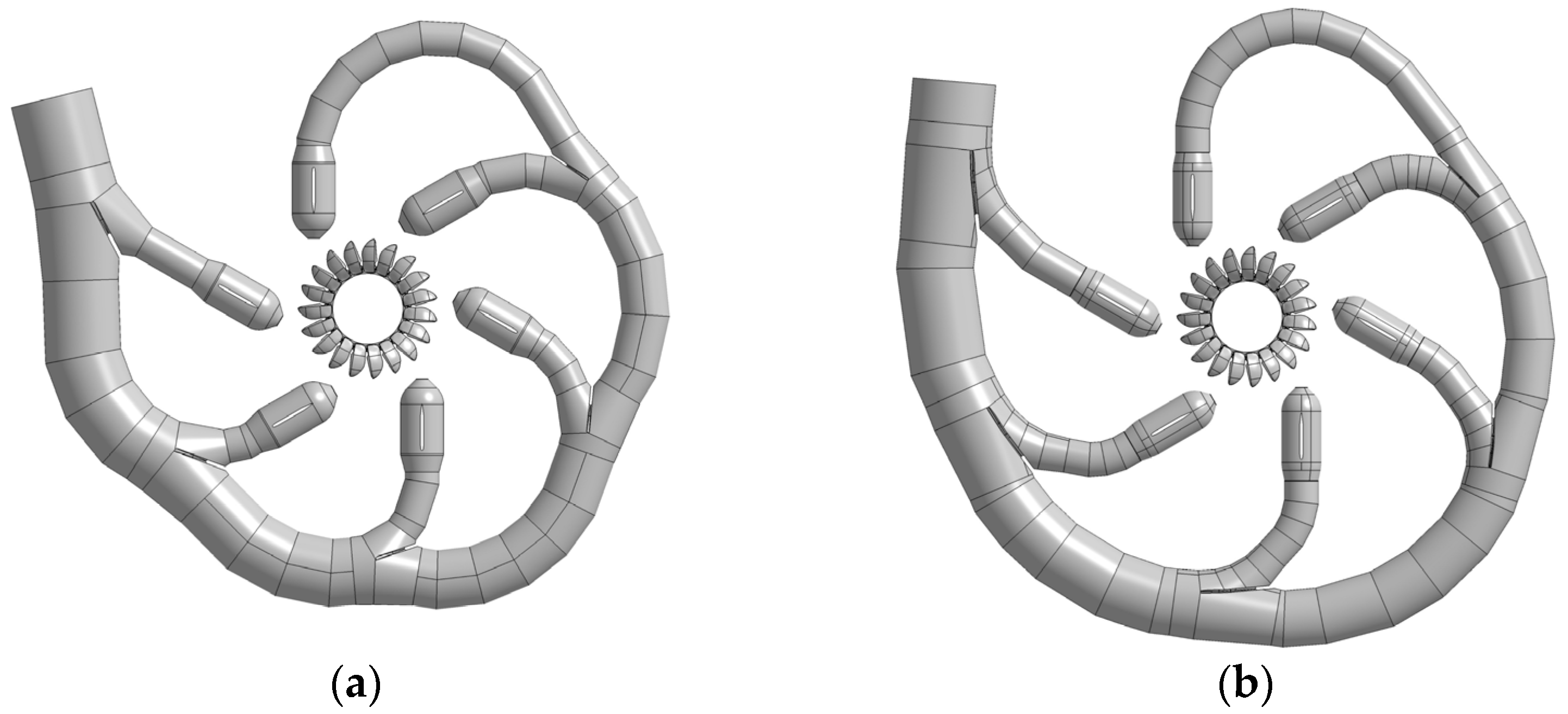
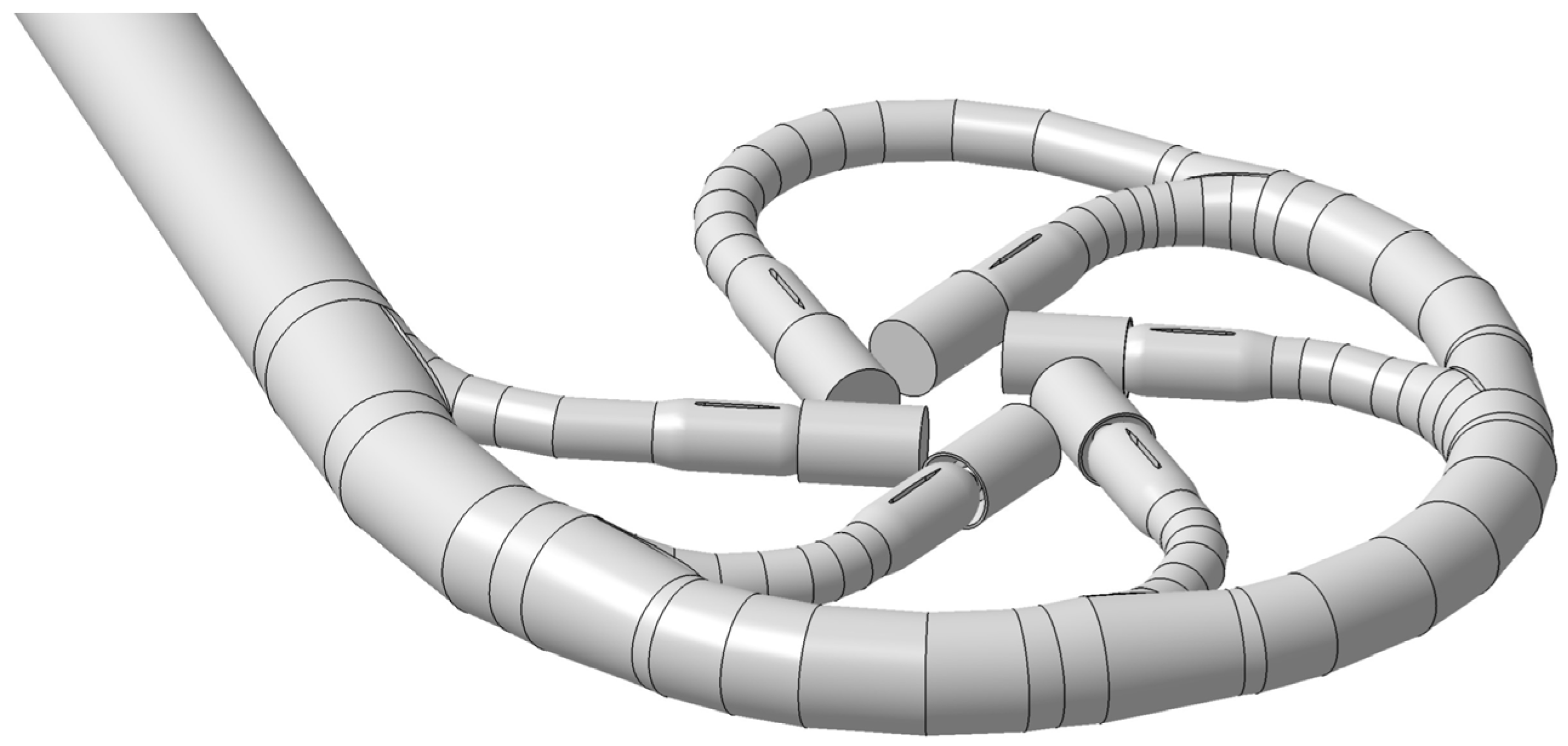
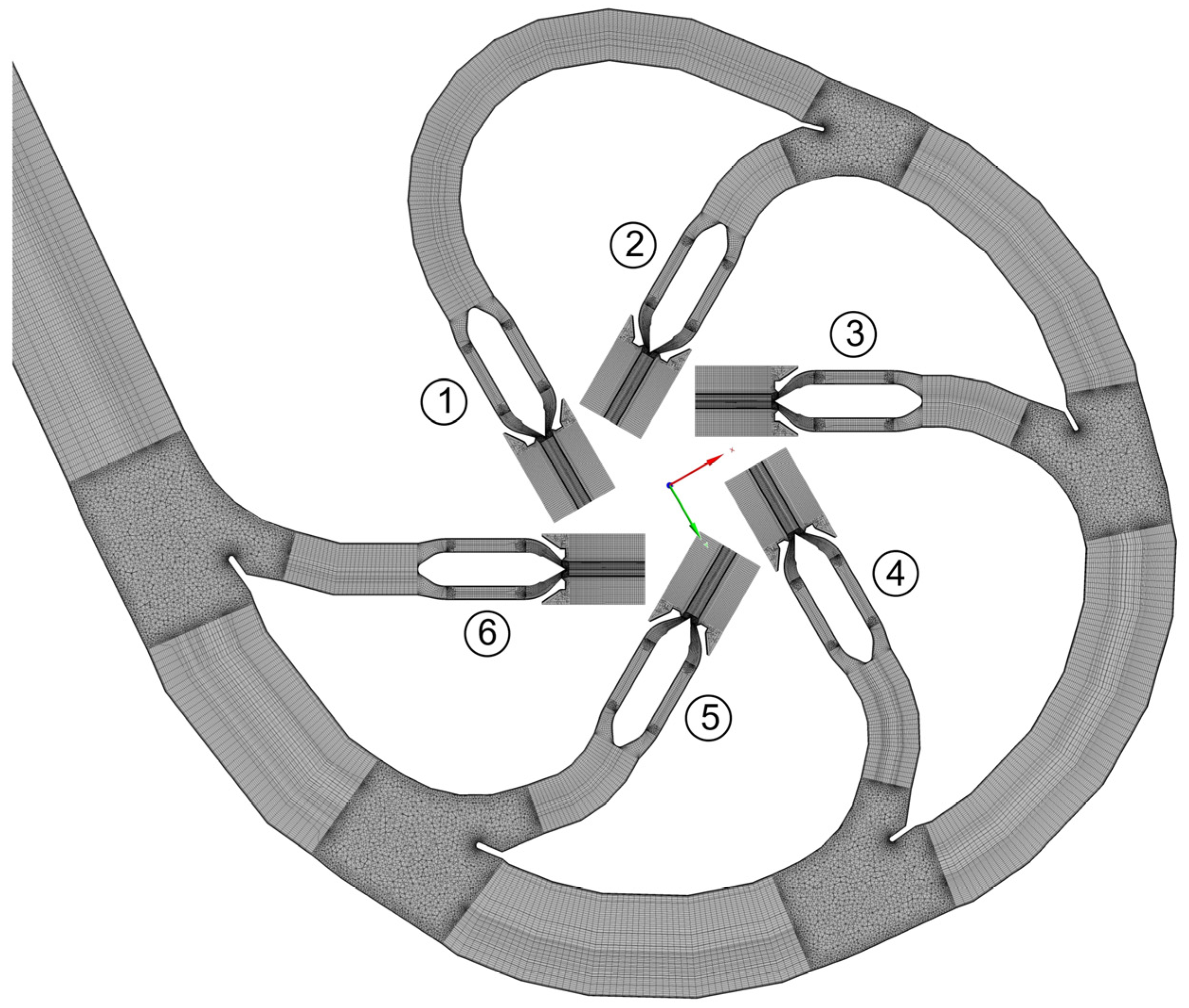
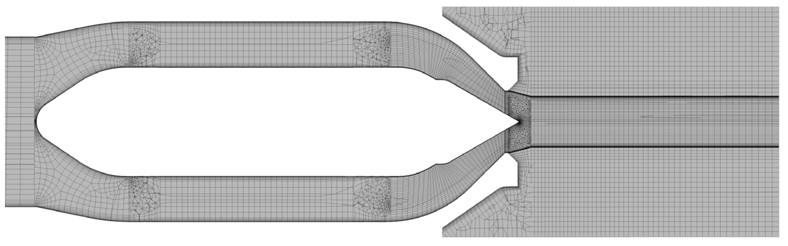
2.2. Numerical Modelling of the Distributor

The modelling of turbulence in the steady-state simulations of the distributor was realised with the k-ω SST model with automatic wall function.
The high-resolution scheme in ANSYS CFX was used to model the advection terms. In addition, relaxation factors for gradient-dependent advection terms were set to enhance numerical stability.
For modelling the two-phase flow, there are two reasonable options, the inhomogeneous model, and the homogeneous model. The first mentioned uses a set of conservation equations for each fluid with specific terms, which model the coupling of the different phases [13]. The higher number of equations results in a better performance compared to the homogeneous model [14]. On the other hand, a higher computational effort is required to solve the equations. The homogeneous model assumes that both fluids share the same flow field. Therefore, only one set of conservation equations needs to be solved with an additional equation, which determines the concentration of each fluid in the gird cells. Thus, a less demanding numerical scheme is necessary than with the inhomogeneous model. The homogeneous model was preferred over the more accurate inhomogeneous model due to higher numerical costs. The selected model also provided a good trade-off between the duration of the simulations and the numerical stability.
Surface tension σ and gravity were not considered in the modelling, which is a common practice and well documented in the literature [4,5,15]. A comparison of both modelling approaches, with and without the consideration of surface tension or gravity, was performed by Židonis in his thesis [5], in which no significant differences in efficiency were shown.
The timestep t was set to 5 × 10⁻⁵ s, which provided a good balance between convergence speed and numerical stability. Additionally, double precision was selected to enhance the stability further.
The geometric model of the distributor was extended by two components. A cylinder with the length of 15 times the inlet diameter was added to the inlet of the distributor. Furthermore, another component was added at the outlets of the nozzles. These volumes correspond to the space in which the jets are formed. Only minor geometric simplifications were made to simplify the numerical modelling.
The geometry shown in Figure 2 represents the basis for spatial discretisation. The final mesh was composed of several blocks of structured and unstructured meshes. Components including rather complex geometry elements, e.g., bifurcations, were meshed with tetrahedral and pyramidal elements. The same mesh topology was used for the leading and the trailing edge of the support ribs in the nozzles and the area of the needle tip. The other elements of the geometry were discretised with structured meshes containing primarily prismatic and hexagonal elements. Along all solid walls, thin layers of prismatic elements were placed.
Figure 3 shows the mesh of the distributor model. In regions of particular interest or with high gradients in relevant flow variables, such as the nozzle exit and the area where the phase boundary of the jet was to be expected, the grid was refined (see Figure 4). Between the mesh components of the distributor and the nozzles general interfaces were placed. The remaining connections between structured and unstructured mesh topologies had a direct mesh connection.
The mesh of the entire simulation domain had about 8.67 million nodes and 14.57 million elements in total. Additional mesh characteristics are summarised in Table 2.
Regarding the boundary conditions, all solid walls of the model were treated as smooth, no-slip walls, without any specific surface roughness defined. The boundary surfaces of the jet domains were modelled as opening boundaries with the relative pressure p rel set to zero, while the reference pressure p ref is equal to the atmospheric pressure p atm . At the inlet a total pressure p tot ,   inlet was imposed with a constant velocity distribution, which corresponds to the given hydraulic head of the turbine.
In order to accelerate the simulation and to increase the numerical stability results of single-phase simulations of the distributor were used to initialise the flow field. At the start of the simulation, the jet domains were filled with air.

2.3. Numerical Modelling of the Runner

In recent publications [9] the k-ω SST model was used for turbulence modelling in Pelton runner simulations. Perrig showed in his thesis [14], that the k-ω SST model outperforms the k-ε model in terms of accuracy. Similar behaviour was summarised in [16]. However, due to significantly, less stable numerical behaviour in runner simulations compared to the distributor simulations, the k-ε turbulence model was applied for the runner simulations. The lack of accuracy of the chosen model is seen as a minor problem since the overall degree of model simplifications is relatively high. Moreover, a relative comparison of different runner geometries, based on identical numerical settings, was not impaired by this.
In analogy to the distributor simulation, the high-resolution scheme was used to model the advection terms. The same relaxation factors as in the study of the distributor were applied. The Second Order Backward Euler scheme was selected for the time discretisation of the transient terms.
Analogous to the numerical modelling of the distributor, the homogenous model was used to model the two-phase flow in the runner. Concerning surface tension and gravity, the same assumption as in the numerical setup of the distributor was made.
The definition of the transient time step t is linked to a discrete angle of runner rotation. The size of the angle-step has been proven as crucial for some factors. A small step provides more stability to the numerical scheme, which leads also to faster convergence behaviour and a lower overall computation time. Both effects have been observed in several simulations. Moreover, the size of the timestep influences the simulation results concerning the torque. The best simulation behaviour was found with a timestep t of approximately 4.63 × 10⁻⁵ s, which corresponds to one-sixth of a degree runner rotation. In the solver settings, double precision was selected to further increase the numerical stability of the simulation.
The runner simulation was based on the geometric model given in Figure 5. The simulation domain is composed of three main components: the runner, the casing, and the nozzles. The former is defined as the rotating domain while the casing and the nozzles remain stationary. The runner is further split into two subdomains, which are indicated by different shadings in Figure 5. Subsequently, these subdomains serve differently in the analysis of the runner’s performance. The medium grey shaded runner component is later used to analyse the performance, while the dark grey component represents some sort of dummy to complement the runner domain. The latter component was necessary to enable the modelling since the combination of six nozzles and 19 buckets did not allow the use of a rotational periodicity for the runner domain. An influence of this component on the results was not given.
To simplify the model, the distributor as well as the real turbine housing were not considered for the simulation. Moreover, the symmetric layout of Pelton turbines was used to further reduce the complexity of the geometric model. This is a common strategy, which is seen in various publications, e.g., [7,10,13]. A non-idealised jet configuration was used. Thus, the last section of the nozzle, the nozzle head, was included in the model to account for the effects of the fluid acceleration and the friction in the spear valve on the jet formation. The nozzle opening was set to 75%, which corresponds to the opening in the nominal operating point of the prototype turbine.
The numerical mesh of the geometry in Figure 5 is composed of components with structured and unstructured meshes (see Figure 6). The nozzles and the casing are represented by a structured mesh of prismatic elements. The two subdomains of the runner were split into two blocks. The first block contains the buckets and was therefore meshed with an unstructured, tetrahedral mesh. The second block of prismatic mesh elements adds up with the first one to complete the rotating runner subdomain. In areas with the strictly aligned flow, such as in the nozzle and jet area, the mesh cells are primarily oriented according to the main flow direction. The cell height in the stationary area was reduced near the sliding surface of the interface. In the rotating domain, no special treatment of the mesh was applied close to the sliding, since the defined cell size was considered sufficiently small. Grid refinements were placed in strategic areas, as shown for the distributor mesh. Near the walls of the runner as well as of the nozzle layers of prismatic elements were placed.
The subdomains of the runner meshed with two different approaches. The one, which incorporates only three consecutive buckets (medium grey shading in Figure 5), was meshed with a comparably high mesh density. The mesh of the other runner subdomain is rather coarse. This approach allows to use of the entire symmetric runner half to be taken into account and yet limits the size of the numerical grid to a manageable number of nodes and elements.
For both subdomains, refinements were placed along the leading edge, the trailing edge as well as the cutout edge and its adjoining surfaces. A detailed view of the refined mesh of the buckets is given in Figure 7. The statistics of the mesh components of the runner simulation are given in Table 3. Quality characteristics of the runner simulation mesh are given in Table 4.
Regarding the boundary conditions, the solid walls of the nozzle and the runner were treated in the same way as those of the distributor, which were modelled as no-slip walls, without any surface roughness defended. A symmetry condition was applied to the symmetry plane of the turbine model. The remaining boundary surfaces were treated with an opening boundary condition since the turbine housing was not considered. The relative pressure p rel is set to zero, while the reference pressure p ref was defined with the atmospheric pressure p atm . Each nozzle has an inlet surface, which is perpendicular to the corresponding nozzle axis. On these a mass flow rate Q inlet normal to the boundary was imposed. The link between the sliding meshes of the rotating runner and the stationary casing was treated with a transient rotor-stator interface.
At the start of the first simulation, a result of a distributor simulation with a corresponding nozzle opening was used to initialise the stationary domain. The rotating domain was filled with air at the start of a simulation run. Subsequent simulations were then initialised with the results of previous transient turbine simulations.

3. Results

3.1. Results of the Distributor Analysis

The simulation of various Pelton distributor geometries in this study showed, that the applied changes to the geometry have led to a reduction of the hydraulic loss in the distributor and improved the flow situation upstream of the nozzles. The latter is important for good jet quality, which is indicated by a circular cross-section and a homogeneous velocity profile of the jet. The main drivers of the deterioration of the jet shape are secondary flows resulting from flow through the curved pipes as they are present upstream of the nozzles. At the exit of the curved pipe, a counterrotating Dean vortex structure forms due to a pressure gradient [17] which causes a stagnation point in the inner core of the pipe resulting in a typical perturbation of the jet cross-section as seen in Figure 8a.
A direct correlation between the jet shape and quantitative flow characteristics is difficult to determine. To overcome this, a swirl number S N was introduced to quantify the intensity of secondary flow. The definition of the S N is given in Equation (1) whereby c circ and c ax are the velocities in circumferential and axial direction respectively on a given plane of the cross-section A .
S N = 1 A · A c circ 2 c ax 2   · d A
For each nozzle, the velocities are referred to the corresponding nozzle axis (positive in jet direction). In the optimisation process of the distributor design, the SN was later used as an additional indicator for an improvement or a deterioration of the jet shape. If the SN decreases, an improvement of the jet shape can be expected, as smaller values indicate a lower intensity of the secondary flows, which primarily act negatively on the jet shape.
Figure 8 shows the cross-section of jet number 4 on a plane about 4.25 jet diameters downstream of the nozzle outlet, which was the jet with the most disturbed jet shape of all. The disturbance of the jet shape in Figure 8 is primarily caused by secondary flows, upstream of the nozzle. The velocity decrease in the boundary region is due to the interaction with air, while in the centre the wake of the needle tip is visible. The wake of the supportive ribs of the nozzle is barely pronounced. The impact of the ribs on the velocity distribution was already significantly reduced in the nozzle head, which can be explained by a strong homogenisation due to the acceleration of the flow in the converging flow channel downstream of the ribs. The jet velocity, which is related to the theoretical velocity c th , is plotted on the cross sections in a range of 0.80 to 1. The boundary of the cross-section is determined by a water volume fraction of 50%. c th is given in Equation (2).
c th = 2 · g · H n
The left plot of Figure 8 corresponds to the baseline geometry of the distributor, and the right plot to the new design. The swirl numbers, which are evaluated at the nozzle inlet, are 0.121 and 0.032 respectively, which is equivalent to a reduction of about 70%. The swirl numbers of the other nozzles are given in Table 5.
Figure 9 shows pressure and the relative velocity in the nozzle exit region which is dominated by strong changes in flow quantities and the flow physics [18] as the flow is accelerated close to c th , the pressure drops accordingly to the atmospheric pressure. The velocity distribution in the symmetry plane of the distributor clearly shows the wake of the needle tip, which remains over the entire length of the jet (see Figure 8).
The hydraulic losses H v in the distributor are determined as a hydraulic head loss from the inlet to the outlet of the corresponding nozzles. H v is given in Equation (3) whereby p ¯ tot ,   Inlet and p ¯ tot ,   Nozzle represent mass flow averaged total pressure values at the inlet and a plane at the nozzle exit. This plane was placed 30 mm upstream from the corresponding nozzle mouthpiece to avoid the influence of flow separation and the changing flow physics of the flow on the result.
H v = p ¯ tot , Inlet p ¯ tot ,   Nozzle ρ · g
These were lowered by roughly 16% compared to the baseline design. A comparison of the head losses, which are related to the nominal head H n , are given in Figure 10. The largest share of the losses was caused by the nozzle, while the distributor contributed less than 20% to the head loss.

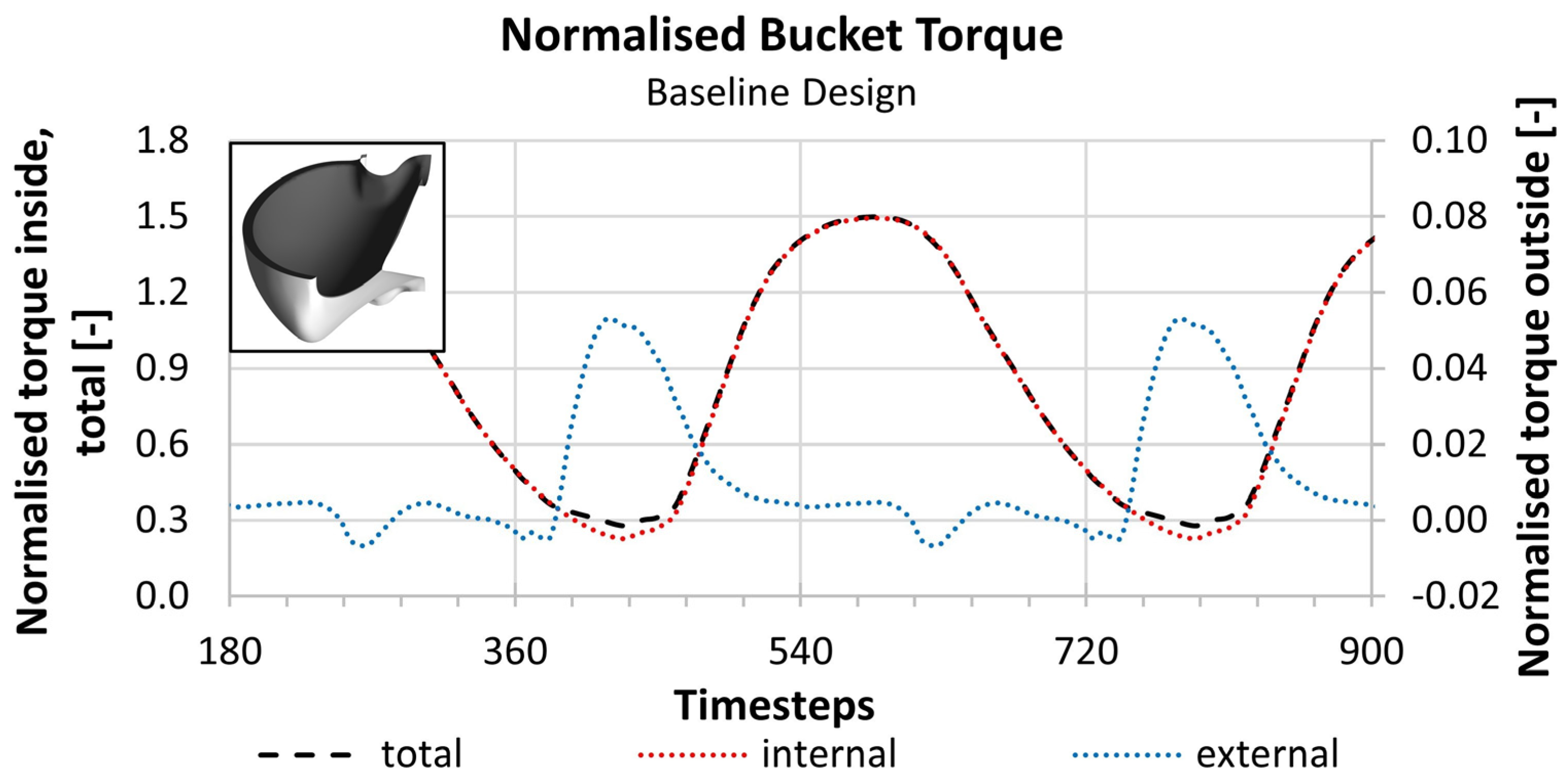
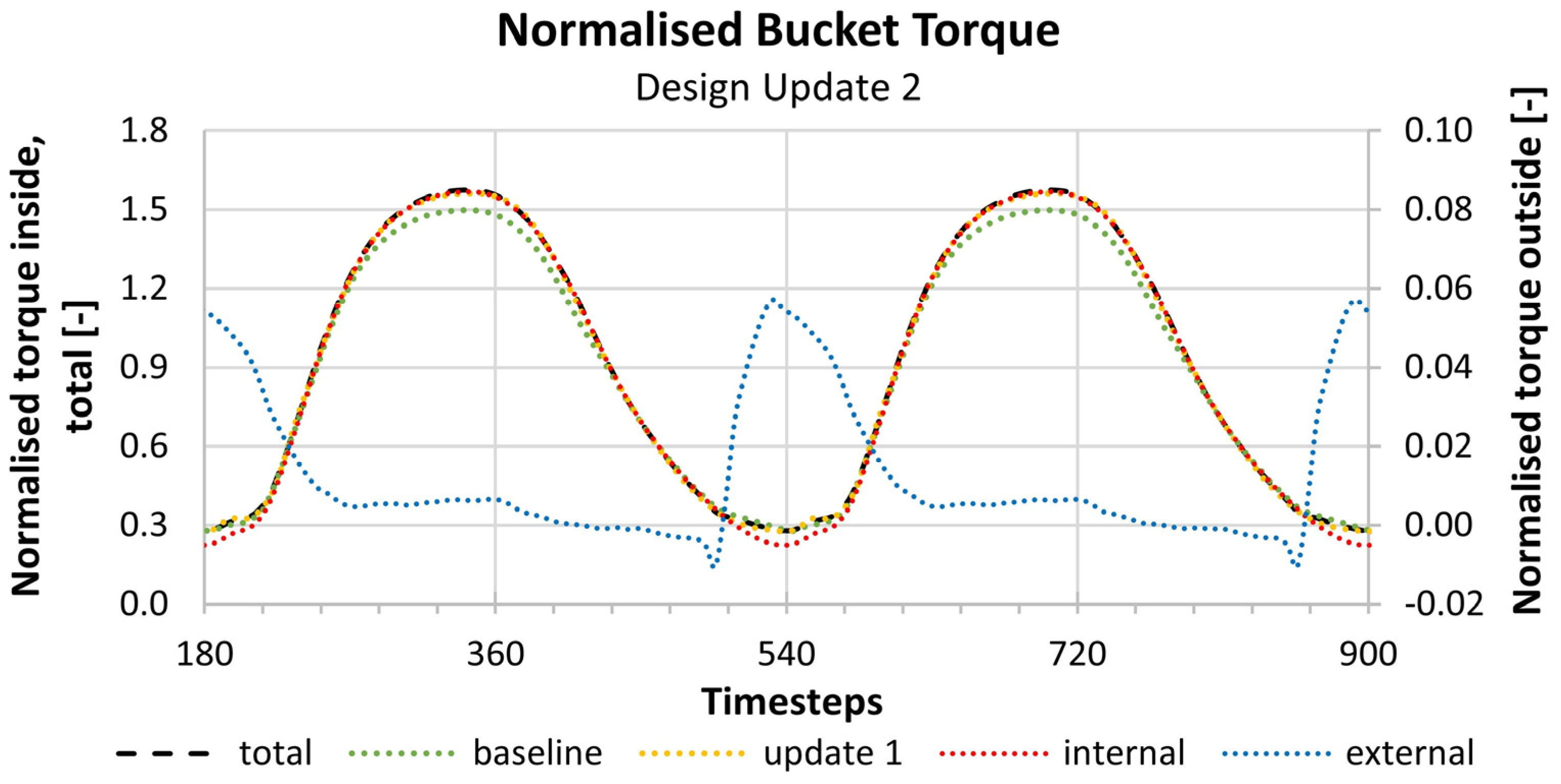
3.2. Results of the Runner Simulation

The results of the three runner simulations, based on different runner geometries, are analysed with a special procedure. For the analysis of the turbine performance in general, a reference bucket was defined. The reference bucket corresponds to the second bucket of the light grey shaded and comparably fine-meshed runner domain in Figure 5. Additionally, to the reference bucket, the leading and the successive bucket are considered to analyse possible, negative interactions on the runner outside surface.
To calculate the runner torque T Runner , a “bucket load cycle” was defined. One load cycle corresponds to what a single bucket experience during 360 timesteps or 60° of runner rotation, since the angular spacing between the nozzles in the case of the present six-nozzle turbine equals 60°. In this period every bucket is once impinged by a jet.
The bucket torque was analysed for each timestep based on the pressure and the wall shear stresses acting on the bucket surface, with pressure values lower than the vapour pressure p vap set to p vap . The limitation of the pressure was necessary to avoid a too high torque contribution, especially from the exterior bucket surface, due to nonphysical pressure values below p vap . The arithmetic average of the torque T ¯ ref over a time span of 360 timesteps or 60° of runner rotation, which is acting on the reference bucket, was finally used to calculate the runner torque. Additionally, T ¯ ref was used as an indicator for the state of convergence of the simulation. A constant level of T ¯ ref indicates a steady-state operation as well as a sufficiently converged solution. The total torque T Runnner of the entire turbine runner corresponds to Equation (4).
T Runner = 2 · T ¯ ref · z
The efficiency η is calculated from T ¯ ref and the corresponding hydraulic head H at the inlets as well as the total imposed flow rate Q at the inlets. The efficiency is given in Equation (5), whereby ω represents the angular velocity of the turbine, ρ the density and g the gravitational acceleration.
η = z · T ¯ ref · ω Q · H · ρ · g
The simulation of the baseline runner design in this study has shown an efficiency of 89.49%. The periodic curve of the generated torque, normalised by T ¯ th for the inside, the outside and the total torque is shown in Figure 11. The splitting of the bucket surface into an interior and an exterior surface is depicted in the upper left-hand corner of Figure 11. The dark grey shaded surface indicates the interior, and the light grey one is the exterior surface. T ¯ th represents a theoretical torque of a bucket based on the simulated head and the flow rate in the nominal operating point with an efficiency of 100%. T ¯ th is given in Equation (6).
T ¯ th = Q n · H · g · ρ 19 · ω
The torque of the primarily impinged interior surface and the exterior bucket surface add up to the torque contribution of the reference bucket. The external curve in Figure 11 indicates the start of the load cycle with its sharp rise after roughly 390 timesteps. A low-pressure zone on the exterior surface causes the growth of the torque in this phase (see Figure 12a). Perrig reported in his thesis the existence of such an external torque and explained it with the Coanda Effect [14].
However, due to non-appropriate trailing edge angles, the same curve shows a loss following timestep 610, which is of significantly lower magnitude due to the smaller area affected and the different orientation of the affected surface. The impingement of the external bucket surface is caused by water, which is exiting the leading bucket. A zone of increased pressure on the exterior surface indicates the source of the loss (see Figure 12b).
The bucket or the runner geometry design was modified to overcome adverse effects in an iterative process, as seen in the results of the baseline geometry simulation. Changes to the bucket width, the trailing edge angles, as well as the splitter and the cutout design have improved the efficiency compared to the baseline runner design. As a result, an efficiency of 90.42% was reached.
Another set of geometry parameters of the Pelton bucket was changed consecutively in a second approach. As a result, the bucket width was slightly increased compared to the first design iteration process, and an increase in the bucket depth was realised. In addition, the positioning of the bucket on the pitch circle diameter was changed towards a smaller bucket position angle. Finally, the leading edge (splitter) and the cutout edge were further altered compared to the first design update. In the end, the numerically calculated efficiency was increased to a level of 90.87% by those measures.
Figure 13 shows the normalised torque of the second design update. Additionally, the total torque of the baseline design and the design update 1 is overlaid (dashed, green and yellow curves, respectively).
In addition to the change of the bucket position angle, the increase in the bucket width and the bucket depth significantly contributed to a remarkable rise in the magnitude of the internal torque compared to the baseline and a small increase compared to the design update 1. On the other hand, the magnitude of the external torque at its maximum remained at a similar level compared to the baseline, which shows a minor impact of the changed bucket position on the external torque. However, the external torque load cycle average is still slightly higher because of the modified trailing edge angles.

4. Conclusions

While the simulation of the Pelton distributor for optimisation is quite common these days, the numerical investigation of the Pelton runner raises more questions.
As presented in this paper, the numerical approach to simulate Pelton runners, primarily of multi-nozzle turbines, should give a direction for an efficient way to analyse their hydraulic behaviour. By focusing on a single reference bucket, especially the numerical grid of the runner domain reduces to a manageable size. Furthermore, with a smaller mesh but still preserving the advantage of a high spatial discretisation in the selected regions, the computational costs and the required simulation time can be reduced significantly. Thus, numerical simulation has come one step closer to possible utilisation for the design and optimisation of Pelton runners.
Within the approach presented, three different Pelton runner designs were analysed with a consistent numerical setup, resulting in efficiencies of 89.49%, 90.42% and 90.87% for the baseline design and two design updates, respectively.
Nevertheless, the calculated efficiencies are partly subject to strong model assumptions and simplifications, such as the non-consideration of the turbine housing, the missing impact of the distributor, and the flow modelling. Therefore, it is essential to point out that the efficiencies given in this paper should not be confused with experimentally determined efficiencies.
In various publications, see e.g., [4,5,10], discrepancies between numerically simulated and experimentally measured efficiencies of Pelton turbines were reported. Whereby over- and underprediction have been shown, primarily depending on the numerical modelling, including mesh density, and physical modelling. Based on this knowledge, the reported efficiency enhancement of 1.38% points between the baseline design and the design update 2 is primarily regarded as an indicator of the actual improvement rather than an absolute value for the efficiency enhancement. Verification of the simulation results still has not yet been conducted based on a model test.

Author Contributions

Conceptualization, L.S. and H.B.; methodology, L.S.; validation, L.S., P.M. and H.B.; formal analysis, H.B.; investigation, L.S.; writing—original draft preparation, L.S.; writing—review and editing, L.S.; visualization, L.S.; supervision, P.M. and H.B.; project administration, L.S.; All authors have read and agreed to the published version of the manuscript.

Funding

This research received no external funding.

Institutional Review Board Statement

Not applicable.

Data Availability Statement

Not applicable.

Conflicts of Interest

The authors declare no conflict of interest.

References

  1. Keck, H.; Sick, M. Thirty years of numerical flow simulation in hydraulic turbomachines. Acta Mech. 2008, 201, 211–229. [Google Scholar] [CrossRef]
  2. Sick, M.; Schindler, M.; Drtina, P.; Schärer, C.; Keck, H. Numerical and experimental analysis of Pelton turbine flow. Part 1: Distributor an Injector. In Proceedings of the IAHR Symposium, Charlotte, NC, USA, 6–9 August 2000. [Google Scholar]
  3. Muggli, F.A.; Zhang, J.; Schärer, C.; Geppert, L. Numerical and experimental analysis of Pelton turbine flow. Part 2: The Free Surface Jet Flow. In Proceedings of the IAHR Symposium, Charlotte, NC, USA, 6–9 August 2000. [Google Scholar]
  4. Zoppé, B.; Pellone, C.; Maitre, T.; Leroy, P. Flow analysis inside a Pelton turbine bucket. J. Turbomach. 2006, 128, 500–511. [Google Scholar] [CrossRef]
  5. Zeng, C.; Xiao, Y.; Luo, Y.; Zhang, J.; Wang, Z.; Fan, H.; Ahn, S.-H. Hydraulic performance prediction of a prototype four-nozzle Pelton turbine by entire flow path simulation. Renew. Energy 2018, 125, 270–282. [Google Scholar] [CrossRef]
  6. Židonis, A. Optimisation and Efficiency Improvement of Pelton Hydro Turbine Using Computational Fluid Dynamics and Experimental Testing. Ph.D. Thesis, Lancaster University, Lancaster, UK, 2015. [Google Scholar]
  7. Rossetti, A.; Pavesi, G.; Cavazzini, G.; Santolin, A.; Ardizzon, G. Influence of the bucket geometry on the Pelton performance. Inst. Mech. Eng. Part A J. Power Energy 2014, 228, 33–45. [Google Scholar] [CrossRef]
  8. Perrig, A.; Avellan, F.; Kueny, J.-L.; Farhat, M.; Parkinson, E. Flow in a Pelton turbine bucket: Numerical and experimental investigations. J. Fluids Eng. 2006, 128, 350–358. [Google Scholar] [CrossRef] [Green Version]
  9. Rentschler, M.; Marongiu, J.C.; Neuhauser, M.; Parkinson, E. Overview of SPH-ALE applications for hydraulic turbines in ANDRITZ Hydro. J. Hydrodyn. 2018, 30, 114–121. [Google Scholar] [CrossRef]
  10. Bhattarai, S.; Vichare, P.; Dahal, K.; Al Makky, A.; Olabi, A.G. Novel trends in modelling techniques of Pelton Turbine bucket for increased renewable energy production. Renew. Sustain. Energy Rev. 2019, 112, 87–101. [Google Scholar] [CrossRef]
  11. Jošt, D.; Mežnar, P.; Lipej, A. Numerical prediction of Pelton turbine efficiency. IOP Conf. Ser. Earth Environ. Sci. 2010, 12, 12080. [Google Scholar] [CrossRef]
  12. Xiao, Y.; Wang, Z.; Zhang, J.; Zeng, C.; Yan, Z. Numerical and experimental analysis of the hydraulic performance of a prototype Pelton turbine. Inst. Mech. Eng. Part A J. Power Energy 2014, 228, 46–55. [Google Scholar] [CrossRef]
  13. Zeng, C.; Xiao, Y.; Wang, Z.; Zhang, J.; Luo, Y. Numerical analysis of a Pelton bucket free surface sheet flow and dynamic performance affected by operating head. Inst. Mech. Eng. Part A J. Power Energy 2017, 231, 182–196. [Google Scholar] [CrossRef]
  14. Santolin, A.; Cavazzini, G.; Ardizzon, G.; Pavesi, G. Numerical investigation of the interaction between jet and bucket in a Pelton turbine. Inst. Mech. Eng. Part A J. Power Energy 2009, 223, 721–728. [Google Scholar] [CrossRef]
  15. Perrig, A. Hydrodynamics of the Free Suface Flow in Pelton Turbine Buckets. Ph.D. Thesis, EPFL, Lausanne, Switzerland, 2007. [Google Scholar]
  16. Židonis, A.; Aggidis, G.A. State of the art in numerical modelling of Pelton turbines. Renew. Sustain. Energy Rev. 2015, 45, 135–144. [Google Scholar] [CrossRef]
  17. Chitrakar, S.; Solemslie, B.W.; Neopane, H.P.; Dahlhaug, O.G. Review on numerical techniques applied in impulse hydro turbines. Renew. Energy 2020, 159, 843–859. [Google Scholar] [CrossRef]
  18. Drazin, P.G.; Reid, W.H. (Eds.) Hydrodynamic Stability; Cambridge University Press: Cambridge, UK, 2010. [Google Scholar]
Figure 1. The layout of the turbine: (a) baseline design; (b) final design.
Ijtpp 08 00010 g001
Figure 2. The geometry of the distributor simulation domain.
Ijtpp 08 00010 g002
Figure 3. Distributor mesh in the symmetry plane with nozzle numbering and global coordinate system.
Ijtpp 08 00010 g003
Figure 4. Mesh of the nozzle and jet area.
Ijtpp 08 00010 g004
Figure 5. Geometric model of the runner simulation domains.
Ijtpp 08 00010 g005
Figure 6. Numerical mesh of casing, nozzles, and the runner.
Ijtpp 08 00010 g006
Figure 7. Detailed view of the mesh refinements: (a) in the internal cutout region; (b) on the external cutout surface.
Ijtpp 08 00010 g007
Figure 8. Improvement of the jet cross-section of nozzle 4: (a) baseline design; (b) design update 2 (both Figures use the same velocity scale).
Ijtpp 08 00010 g008
Figure 9. Velocity and pressure distribution at the nozzle exit: (a) relative velocity; (b) pressure.
Ijtpp 08 00010 g009
Figure 10. Comparison of the relative headloss.
Ijtpp 08 00010 g010
Figure 11. Normalised torque (baseline design).
Ijtpp 08 00010 g011
Figure 12. Pressure distribution on the runner exterior surface of the baseline design; (a) low pressure on the external cutout surface; (b) increased pressure on the lateral exterior bucket surface.
Ijtpp 08 00010 g012
Figure 13. Normalised torque (design update 2 vs. baseline and design update 1).
Ijtpp 08 00010 g013
Table 1. Main dimensions of the turbine.
Characteristic DimensionsValues
D 1310.00 mm
B 375.25 mm
d 0 115.00 mm
D / B 3.50
z 19
Table 2. Distributor mesh quality characteristics.
Mesh MetricMinimumMaximumAverage
Min. Face Angle11.3°90.0°57.8°
Max. Face Angle60.0°157.3°97.2°
Aspect Ratio135124.1
Y Plus--41.1
Table 3. Mesh statistics of the casing and the runner subdomains (in millions).
Mesh RegionNodesElements
Nozzle, Casing2.6042.352
Runner fine4.53017.101
Runner coarse5.59716.511
Total12.73235.965
Table 4. Runner mesh quality characteristics.
Mesh MetricMinimumMaximumAverage
Min. Face Angle10.4°90.0°47.9°
Max. Face Angle60.0°153.2°92.5°
Aspect Ratio12266.3
Y Plus--53.1
Table 5. Comparison of the swirl numbers for the distributor.
DesignNozzle 1Nozzle 2Nozzle 3Nozzle 4Nozzle 5Nozzle 6
Baseline Design0.0270.0390.0410.0320.0360.023
New Design0.0570.1150.0690.1210.0870.065
Disclaimer/Publisher’s Note: The statements, opinions and data contained in all publications are solely those of the individual author(s) and contributor(s) and not of MDPI and/or the editor(s). MDPI and/or the editor(s) disclaim responsibility for any injury to people or property resulting from any ideas, methods, instructions or products referred to in the content.

