


Relation between PM2.5 and O3 over Different Urban Environmental Regimes in India
by
 , , , , ,
Rahul Kant Yadav
1 ,
,
Harish Gadhavi
2,
Akanksha Arora
2,3,
Krishna Kumar Mohbey
4,
Sunil Kumar
4,5,
Shyam Lal
2 and
Chinmay Mallik
1,* 1
Department of Atmospheric Science, Central University of Rajasthan, Ajmer 305801, India
2
Space and Atmospheric Science Division, Physical Research Laboratory, Ahmedabad 380009, India
3
Department of Physics, Indian Institute of Technology Gandhinagar, Gandhinagar 382055, India
4
Department of Computer Science, Central University of Rajasthan, Ajmer 305801, India
5
School of Business, Woxsen University, Hyderabad 502345, India
*
Author to whom correspondence should be addressed.
Urban Sci. 2023, 7(1), 9; https://doi.org/10.3390/urbansci7010009
Submission received: 5 December 2022
/
Revised: 9 January 2023
/
Accepted: 10 January 2023
/
Published: 17 January 2023
(This article belongs to the Special Issue Urban Climate Change Management and Society)
Abstract
:Atmospheric ozone (O3) concentration is impacted by a number of factors, such as the amount of solar radiation, the composition of nitrogen oxides (NOx) and hydrocarbons, the transport of pollutants and the amount of particulate matter in the atmosphere. The oxidative potential of the atmosphere and the formation of secondary organic aerosols (SOAs) as a result of atmospheric oxidation are influenced by the prevalent O3 concentration. The formation of secondary aerosols from O3 depends on several meteorological, environmental and chemical factors. The relationship between PM2.5 and O3 in different urban environmental regimes of India is investigated in this study during the summer and winter seasons. A relationship between PM2.5 and O3 has been established for many meteorological and chemical variables, such as RH, WS, T and NOx, for the selected study locations. During the winter season, the correlation between PM2.5 and O3 was found to be negative for Delhi and Bengaluru, whereas it was positive in Ahmedabad. The city of Bengaluru was seen to have a positive correlation between PM2.5 and O3 during summer, coinciding with the transport of marine air masses with high RH and low wind speed (as evident from FLEXPART simulations), leading to the formation of SOAs. Further, O3 concentrations are predicted using a Recurrent Neural Network (RNN) model based on the relation obtained between PM2.5 and O3 for the summer season using NOx, T, RH, WS and PM2.5 as inputs.
1. Introduction
It is well known that the photochemical production of tropospheric O3 is determined by the ambient levels of its precursors, such as the oxides of nitrogen (NOxs) and volatile organic compounds (VOCs). The rate of photolysis depends on the meteorological parameters (such as temperature and solar radiation) as well as the chemical parameters [1]. O3, being an atmospheric oxidant, can also lead to the formation/growth of particles in the atmosphere. Aerosols also play an important role in O3 production as they interact with radiation through scattering and absorption and, therefore, affect atmospheric radiation and temperature. The aerosol-induced reduction in solar irradiance was estimated to result in lower photolysis rates and less production of O3 in the Eastern Mediterranean region [2].
The relationship between O3 and PM2.5 in the summer and winter seasons was studied over Nanjing–Jiangsu Province’s capital city in eastern China, and it was observed that O3 and PM2.5 showed inverse relations during the summer and winter seasons [3]. Analysis of environmental and meteorological measurements for three years over Nanjing shows that the two dominant processes have identified basic pathways for interactions between two important atmospheric pollutants, viz., PM2.5 and O3.
- Secondary particle production gets enhanced by high O3 concentrations and strong atmospheric oxidation, raising ambient PM2.5 levels.
- Increased PM2.5 concentrations might lower the ambient O3 levels by reducing atmospheric radiation.
The formation of secondary particles is promoted in the summer season due to enhanced solar radiation and strong atmospheric oxidation. During winter, high concentrations of PM2.5 reduces solar radiation, which inhibits the synthesis of O3, which may result in a negative relationship between ambient PM2.5 and O3. Seasonally altering interactions between PM2.5 and O3 could be determining factors in the seasonal variations in air pollution. The interaction between PM2.5 and O3 is mainly affected by photochemical reactions [4] and secondary organic and inorganic aerosols generated from oxidation reactions consisting of a significant fraction of particulate matter, with substantial implications for air pollution [5].
The relationship between O3 and PM2.5 depends on many meteorological factors, such as temperature, relative humidity (RH) and wind speed (WS). RH plays an important role in secondary particle formation and related chemical and physical properties [6]. Kaul et al. (2011) [7] observed enhancement in secondary organic aerosol (SOA) concentrations under high RH conditions. The effects of RH on the formation of SOAs have been investigated through both chamber studies and ambient measurements [6], yet the knowledge of SOA formation under different RH conditions is rather limited. Zang et al. (2014) [8] examined the reaction of aerosol pollution in Wuhan city in China during wintertime and found that aerosol pollution in Wuhan is dominated by PM2.5 on wet days (RH 60%). The aqueous chemistry is favoured by enhanced RH. Increased RH also aids in new molecule development and the deliquescence development of pre-existing particles, which may prompt an increment in aerosol concentration. While studying the changes in the AOD due to the lockdown imposed in India to restrict the spread of the coronavirus disease (COVID-19), it was found that the area-average AOD increased with increasing RH in central India during the lockdown period [9,10].
SOA is mostly formed by the oxidation of volatile organic compounds (VOCs), the products of which present sufficiently low volatility to partition into the particle phase, according to the gas-particle partitioning theory [11], and, afterwards, nucleate and form organic particles. Hydroxyl (OH) radicals, O3, and nitrate (NO3) radicals are the three major oxidants in the atmosphere that react with organic gases to form SOAs. Among these, data for O3 is easily available over wide geographic areas, including India. Guo et al. (2017) [12] observed that SOAs contributed a minuscule of 7% and 3% to PM2.5 over Jaipur and Delhi, respectively, in 2015. Behera and Sharma (2010) [13] calculated that the SOAs in Kanpur city in the Indo-Gangetic Plain (IGP) account for around 18% of PM2.5 in the winter and 12% of PM2.5 in the summer. In Delhi and nearby regions, SOAs were found to contribute 16 ± 6 µgm−3, which accounts for up to 5.8 ± 2.6% of the PM2.5 mass in summer [14].
In this study, we make an attempt to find the relationship between PM2.5 and O3 under different meteorological and chemical factors such as RH, WS, temperature and NOx over climatically contrasting urban environmental regimes in India, viz., Delhi in north India, Ahmedabad in western India and Bengaluru in south India (Section 1.1). An attempt is made here to predict the ozone concentrations over the selected study locations using the Recurrent Neural Network (RNN) model.
1.1. Study Locations
Delhi: Delhi (28.70° N, 77.10° E), the capital of India, has severe air pollution issues. In October 2018, the Ministry of Earth Science, India, issued a study attributing over 40% of PM2.5 air pollution in Delhi to vehicle exhaust, 22% to dust/fire and 20% to industry. From January to September, Delhi has records of air quality of Large Moderate (101–200) levels, followed by a radical decrease between the months of October and December to Very Poor (301–400), Severe (401–500) and Hazardous (500+) levels because of several variables, including stubble consumption, Diwali fireworks and other festivals and a chilly climate. As indicated by a study on Delhi air contamination by Rizwan et al. (2013) [15], the rising air pollution level has increased the number of cases related to respiratory diseases (particularly asthma and cellular breakdown in the lungs), hypertension, chronic headache, eye irritation and skin irritation. In Delhi, during wintertime, the dense brown haze and murkiness constantly cause major problems in aviation and train transport.
Ahmedabad: Ahmedabad (23.02° N, 72.57° E), situated on the bank of river Sabarmati, is a prominent city in Gujarat. There has been a fast development of enterprises in the city; in particular, drugs, petrol and petrochemical ventures, steel reuse, car parts fabrication, drinks creation, and material creation are the major contaminating businesses concerning air pollution. Ahmedabad city is growing quickly, and vehicular traffic and enterprises are additionally expanding. These advancements are increasing the atmospheric aerosol concentration, which, in turn, increases ambient air pollution substantially. This increase in air pollution has a negative impact on the environment as well as on the health of people living in Ahmedabad.
Bengaluru: Bengaluru (12.97° N, 77.59° E) is one of the principal information technology (IT) centres of India. Bengaluru is known for its wonderful and consistent climate. The city is situated 920 m above sea level, and it is the most elevated city among the significant urban areas in India. The coolest month is January, with a normal low temperature of 15.1 °C, and the hottest month is April, with a normal high temperature of 35 °C. Bangalore gets precipitation from both upper-east and southwest storms. Bengaluru is broadly viewed as the “Silicon Valley” of India. Fast urbanisation has altered the city’s land use and land cover features, particularly in the eastern sections, which are home to major IT parks such as Whitefield and Electronic City. The city’s economic development has resulted in an increase in population and the number of vehicles on the road. Guttikunda et al. (2019) [16] assessed the emissions for the year 2015 in Bengaluru city to be 31,500 tons of PM2.5, 67,000 tons of PM10, 5500 tons of SO2, 57,000 tons of NOx, 335,600 tons of CO, and 84,000 tons of non-methane volatile organic compounds (NMVOCs).
1.2. Emissions
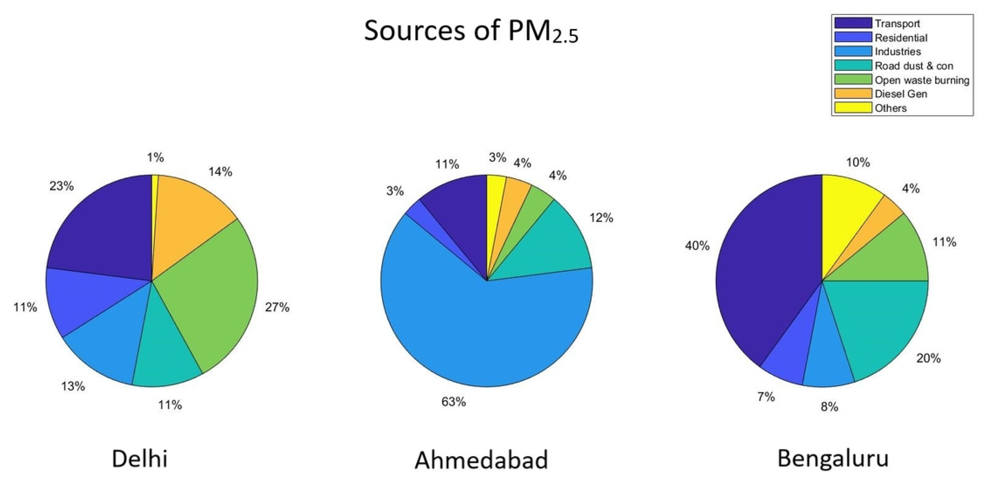
Emissions of pollutants comprising particulate matter (aerosols) and gases (NO2 and CO) play a vital role in the environment and human health [17]. The most commonly identified sources of primary air pollutants comprising particulate matter (aerosols) and gases (NO2 and CO) are vehicular emissions, power generation, manufacturing industries, construction, road dust, open waste burning, oil and coal combustion, and household activities. Figure 1 shows the source apportionment of PM2.5 for three cities in India based on data from URBAN emissions.info sourced from APnA “Air Pollution Knowledge Assessment” city program [16]. In Delhi, a major source of PM2.5 is open waste burning (27%), followed by emissions from vehicles (23%). Emissions from industries dominate the PM2.5 sources in Ahmedabad (63%), whereas vehicular emission is one of the major sources of PM2.5 in Bengaluru, contributing 40%.
In India, 45% of the total NOx emissions come from coal burning in thermal power plants and 32% comes from road transport. [18]. However, O3 being a secondary pollutant, changes in O3 would be much more difficult to unravel from direct observations, and the dependency on hydrocarbons, NOx and meteorological factors needs to be investigated. Coincidentally, xylenes were found to be the largest contributor to O3 formation, followed by toluene in Delhi [19]. Chen et al. (2020) [20] pointed out that O3 production is less sensitive to solar radiation in summer compared to winter. Reducing NOx by itself raises O3, thus reducing NOx emissions by 50% leads to a 10–5% rise in surface O3, and, conversely, decreasing VOC emissions can lessen O3 effectively, to such an extent that a half decrease in VOC emissions will lead to a 60% decrease in O3 in Delhi [20].
2. Materials and Methods
2.1. Data
For this study, based on long-term data availability and contrasting climatic conditions, three stations were selected: Ahmedabad, Delhi and Bengaluru. The air quality data for the selected cities have been taken from the Central Pollution Control Board (CPCB) of India. The PM2.5, O3 and NOx data were downloaded from the CPCB website. With the aid of State Pollution Control Boards and other organisations under the National Air Quality Monitoring Programme (NAMP), the CPCB monitors air quality across 233 stations throughout the Indian region (http://cpcb.nic.in/air.php, accessed on 10 March 2021). Daily metrological data (relative humidity (RH), temperature (T) and wind speed (WS)) from the years 2010 to 2020 was taken from the NASA/POWER (Prediction of Worldwide Energy Resource) project (https://power.larc.nasa.gov/data-access-viewer, accessed on 10 March 2021). The POWER Data Archive provides global data at a resolution of 0.5 x 0.5 degrees in CSV, ASCII and NetCDF. Data used in this study were downloaded in CSV format. For the POWER project, NASA’s Modern-Era Retrospective Analysis for Research and Applications version 2 (MERRA-2) assimilation model and GEOS 5.12.4 FP-IT were used to determine meteorological parameters [21]. MERRA-2 is based on the Goddard Earth Observing System (GEOS) Data Assimilation System, while GEOS 5.12.4 has similar grid resolution and model physics to MERRA-2, with some exceptions [22]. The POWER project team processes GEOS 5.12.4 data on a daily basis and combines it with the MERRA-2 daily time series to create low-latency products that are usually available within two days in real-time. The air mass trajectory was calculated using web-based HYSPLIT. The planetary boundary layer (PBL) height was extracted from the HYSPLIT model simulation results.
The data for 6 parameters were extracted for this study (also available as Supplementary Material).
- (i)
- Particular matter (PM) of aerodynamic diameter less than 2.5 μm (PM2.5);
- (ii)
- Ozone (O3);
- (iii)
- Nitrogen oxides (NOx);
- (iv)
- Relative humidity (RH);
- (v)
- Temperature (T); and
- (vi)
- Wind speed (WS).
The measurement techniques for O3, NOx and PM2.5 are available from the technical specifications for Continuous Ambient Air Quality Monitoring (CAAQM) (CPCB, 2019, https://cpcb.nic.in, accessed on 10 March 2021). The ultraviolet photometric O3 gas analysers work on Beer Lambert’s principle on the absorption of radiation at 254.7 nm by atmospheric O3. With a response time of 30 s or less, the instrument’s detection limit is 1 ppb. For the measurement of NOx, nitric oxide (NO) is oxidised by O3 molecules to produce chemiluminescence, which peaks at 630 nm radiation [23]. With the aid of a molybdenum converter, NO2 is converted into NO, which is then used to calculate the total amount of NOx. Unfortunately, other nitrogen species are also reduced to NO and interfere with the measurement of NO2 because the reduction of NO2 to NO is not unique to NO2. These instruments have detection limits of approximately 1 ppb at response times of 120 s or less. The PM10 measurements are based on the principle of β-ray attenuation. At a flow rate of 16 l/min, the instrument samples ambient air for particulate matter, which is then collected on fibreglass filter tape. The amount of PM10 is determined by comparing scintillation/G.M. counter measurements of β -ray radiation taken before and after sampling. The particle size cut-off for PM2.5 is in the range of 0–2.5 μm, but the measurements are similar to those for PM10.
The raw data (CPCB data) were filtered station-wise and species-wise to remove values above and below 3 standard deviations from the mean at every one-month interval. Since we are concerned with the average variation of the pollutants, this kind of filtering helps to remove bias due to extreme events (meteorological or chemical) and errors related to instruments, sampling and human effects. Additionally, data were also checked manually for inconsistencies. This paper studies the relationship between O3 and PM2.5 during the summer and winter seasons. The winter days selected here are from 1 December to 14 February and the summer days are from 1 March to 31 May. Table 1 presents the basic statistical measures, including the mean, median, and standard deviation, as well as other statistical parameters for the data during the summer and winter seasons. At first, the relationship between O3 and PM2.5 was observed by finding the regression between them during the summer and winter seasons. Additionally, the regression for the different ranges of meteorological (RH, WS and T) and chemical parameters (NOx) were studied to find the dependence of PM2.5 and O3 on those meteorological parameters during both winter and summer seasons. The dependence was tested for different levels of significance using a two-tailed Student’s t-test. For better and improvised results, the binning average for O3 was calculated for each station and the regression was observed for all the above-mentioned conditions.
2.2. Lagrangian Particle Dispersion Model: FLEXPART
We used the Lagrangian particle dispersion model (LPDM) FLEXPART v10.4 [24,25,26] for this study. There are different varieties of dispersion models in use in the scientific community. The best model for a given problem depends on factors such as spatial and temporal scales, computational efficiency, and the representation of complex processes such as the effect of topography, chemistry, meteorology, etc. Leelossy et al. (2014) [27] discussed the merits and demerits of different types of dispersion models under different conditions, e.g., in the ground-level air pollution model (GLAMP), the local surface airflows differ significantly from the general meteorological dataset as wind speed less than 6 m/s is set to 6 m/s, rendering it unacceptable for many cities. Lagrangian dispersion models stand out for their applicability in a wide range of situations, computational efficiency and low numerical diffusion. They are used to simulate source–receptor relationships from the scale of a city to the continents [28,29,30,31,32]. FLEXPART is an open-source model that allows several publicly available reanalysis meteorological data products or model outputs as input to compute the trajectories of a large number of particles (infinitesimally small air parcels). FLEXPART incorporates several particle dispersion and removal mechanisms, such as diffusion by turbulence, dry deposition, wet deposition, and deep convective mixing [33]. The fact that FLEXPART involves chemistry gives it an edge over GRAL, which does not support chemical reactions and transformations between substances [28]. FLEXPART can run in both forward and backward in-time modes. When used in backward mode, unlike simple back-trajectory models, it provides quantitative values that represent the source–receptor (S-R) relationship and are related to the residence time of particles in output grid cells. Thus, the S-R relationship, so calculated, is simply a matrix describing the sensitivity of a receptor to geographically distributed sources, also known as potential emission sensitivity (PES). A more thorough explanation of PES values and the S-R relationship can be found in Seibert and Frank (2004) [33].
In our study, we employed FLEXPART backward modelling to simulate the transport and dispersion of secondary organic aerosol (SOA). The receptors are 24 h averaged SOA concentration observations in Bengaluru for different days, and the sources are area-averaged SOA emissions from various grid boxes at different intervals. The model was run using NCEP FNL (Final) Operational Global Analysis data. The spatial resolution of FNL input files is 1° X 1°, with 26 vertical levels, ranging from the surface to 10 millibars, and a time resolution of 6 h. For each date and the receptor sites, 40,000 particles were released. Assuming no direct emissions at higher altitudes, potential emission sensitivity is calculated for the bottom 100 m layer, known as the footprint layer, for a backward time of 10 days.
2.3. Recurrent Neural Network (RNN)
To predict the O3 concentration, a Recurrent Neural Network (RNN) model has been used. RNNs [34,35,36] are a class of artificial neural networks that have an internal state or short-term memory due to their recurrent feedback connections. Therefore, these networks are suitable for sequential problems such as speech classification and prediction and generation. The Recurrent Neural Network (RNN) [37] model has been successfully applied to sequence learning and pattern recognition [38] and scene labelling [39]. In contrast to feed-forward networks such as CNNs, RNNs have recurrent connections in which the previous hidden state informs subsequent hidden states.
where xt ∈ RM and ht ∈ RN are the entry and hidden states, accordingly, at step t. The weights for the present and recurrent inputs and the bias of the neurons are W ∈ RN × M, U ∈ RN × N and b ∈ RN. An RNN layer consists of N neurons, and σ is an element-level activation function of the neurons.
ht = σ (Wxt + Uht−1 + b)
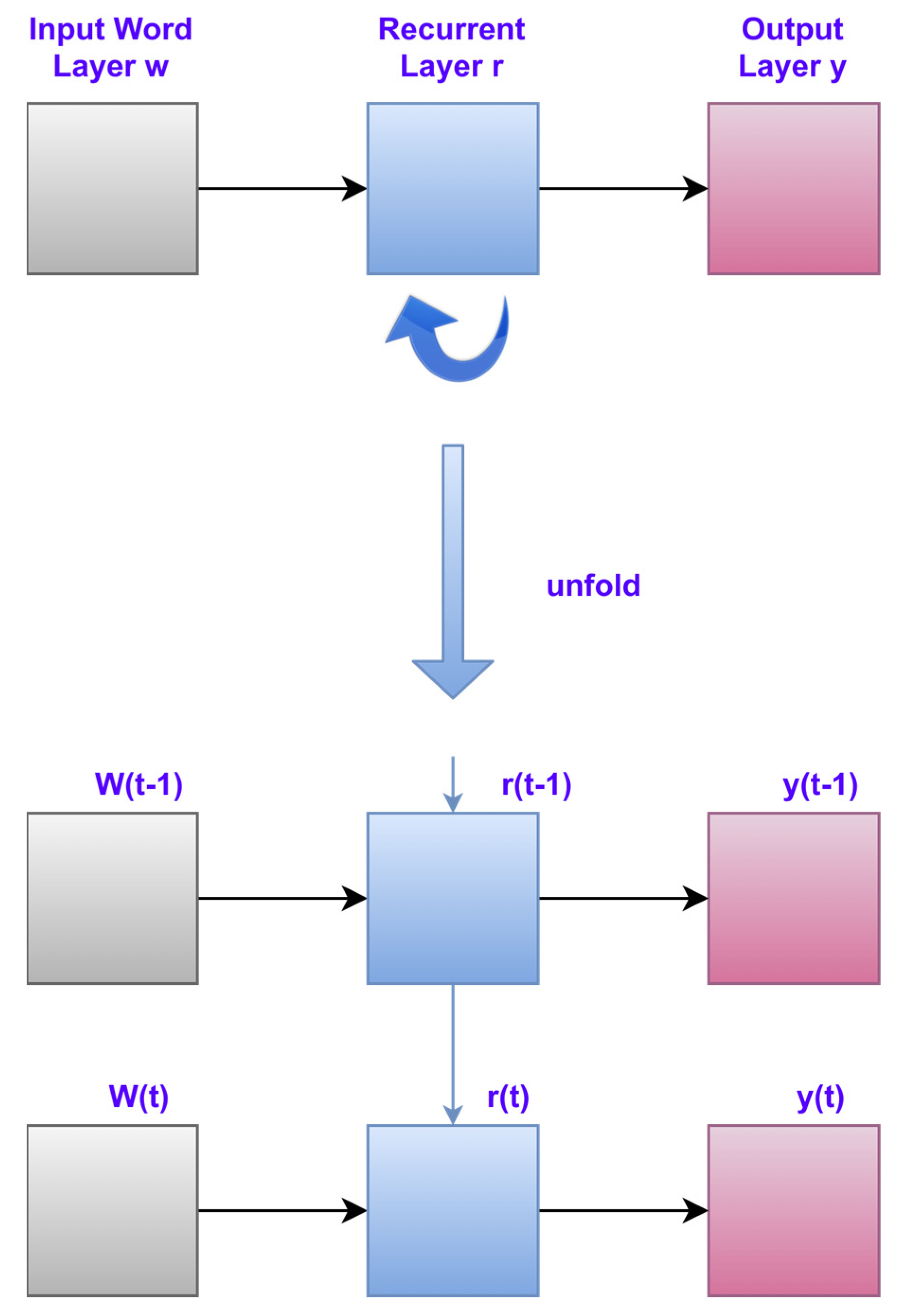
Its structure is seen in Figure 2. Each time frame is made up of three layers: three input word levels w, one recurrent layer r and one output layer y. The activation of the input, recurrent, and output layers at time t is represented by W(t), r(t) and y(t), respectively. Mikolov et al. (2010) [40] defined w(t) as the current word vector, which can be a simple 1-of-N coding representation h(t) (i.e., the binary one-hot representation with the same dimension as the vocabulary size but only one non-zero element). The following formula may be used to calculate y(t):
where x(t) is a vector formed by concatenating w(t) and r(t1), f1(.) and g1(.) are sigmoid and softmax functions, respectively, and U, V are learned weights. The RNN’s size adjusts to the length of the input sequence. In various time frames, the recurrent layers connect the sub-networks. As a result, we must propagate the mistake back in time using recurrent connections [41]. Figure 2 depicts the recurrent neural network design. A loss function related to MSE was minimised by optimising the model parameters. Keras was used to do the optimisation, utilising ADAM. We experimented with several RNN designs, changing the number of layers, filters per layer, the kind of layer (hidden or dense), and the filter size. The models were trained throughout 50 epochs using an early-stopping set. RNN model architecture and configurations are shown in Figure 3.
x(t) = [w(t) r(t − 1)];
r(t) = f1(U · x(t));
y(t) = g1(V · r(t));
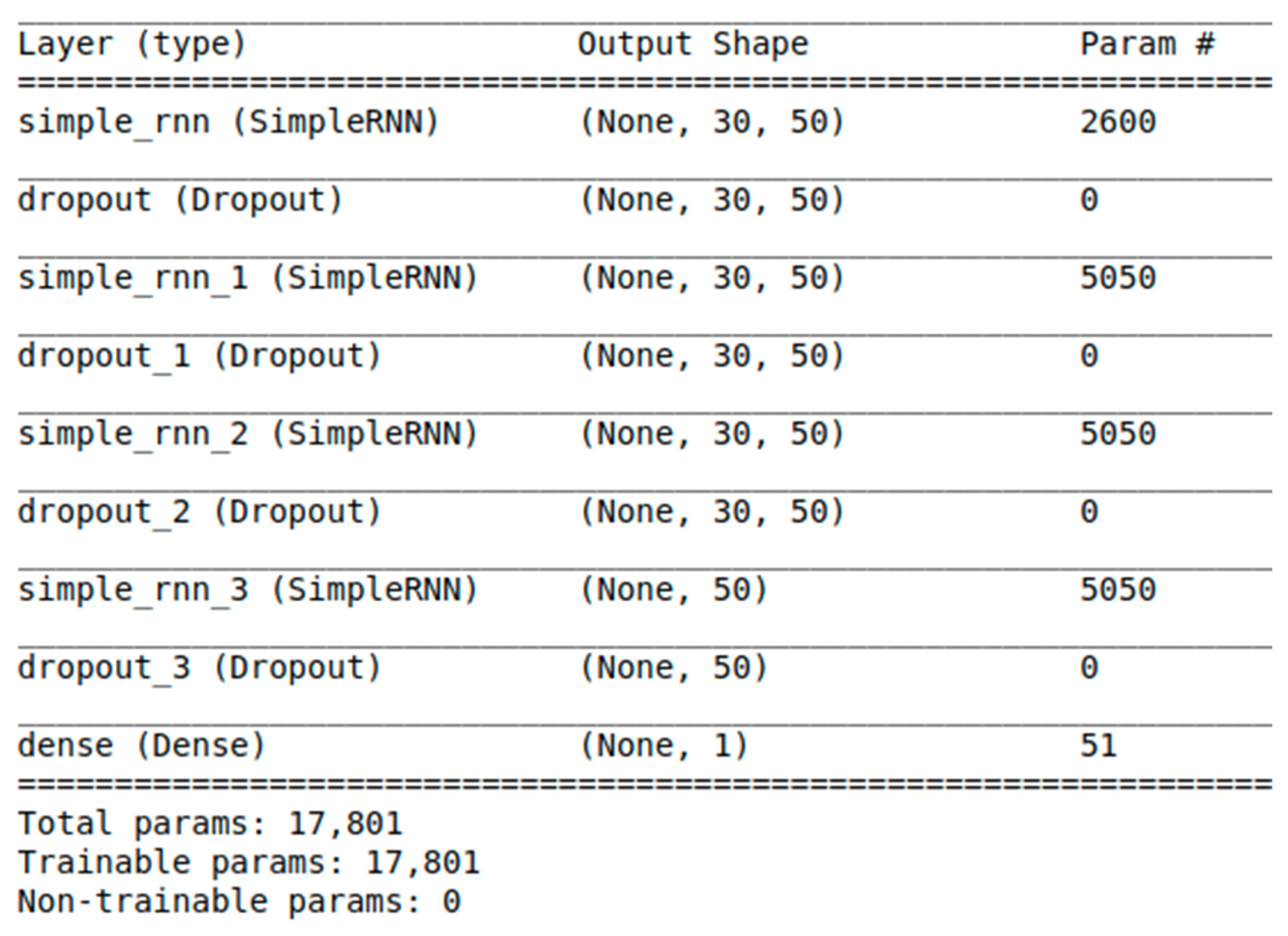
Figure 3 shows the architecture of our RNN model and the associated configuration parameters. The RNN model architecture consists of four SimpleRNN layers, four dropout layers, and one dense layer. SimpleRNN is a fully connected RNN where the output from the previous timestep is to be fed to the next time step. The input image is (638 × 30), and the image first goes to the first SimpleRNN layer. The first layer has four inputs, a 50-dimensional output space, an activation function called Swish, a return sequence called True, and an input shape. Then, a dropout with a probability of 0.2 is applied. Its function is to reduce the spatial size of the incoming entities and, thus, contribute to reducing the number of parameters and calculations in the network, thus helping to reduce over-learning. The second, third, and fourth SimpleRNN layers also have 50 dimensionalities of the output space and a dropout of 0.2. The architecture ends with a dense layer. Table 2 includes information about the hyperparameter, which we used to tune the performance of this model, such as learning rate, hidden layers, dropout value, batch size, epochs, activation functions, and optimiser.
3. Result and Discussion
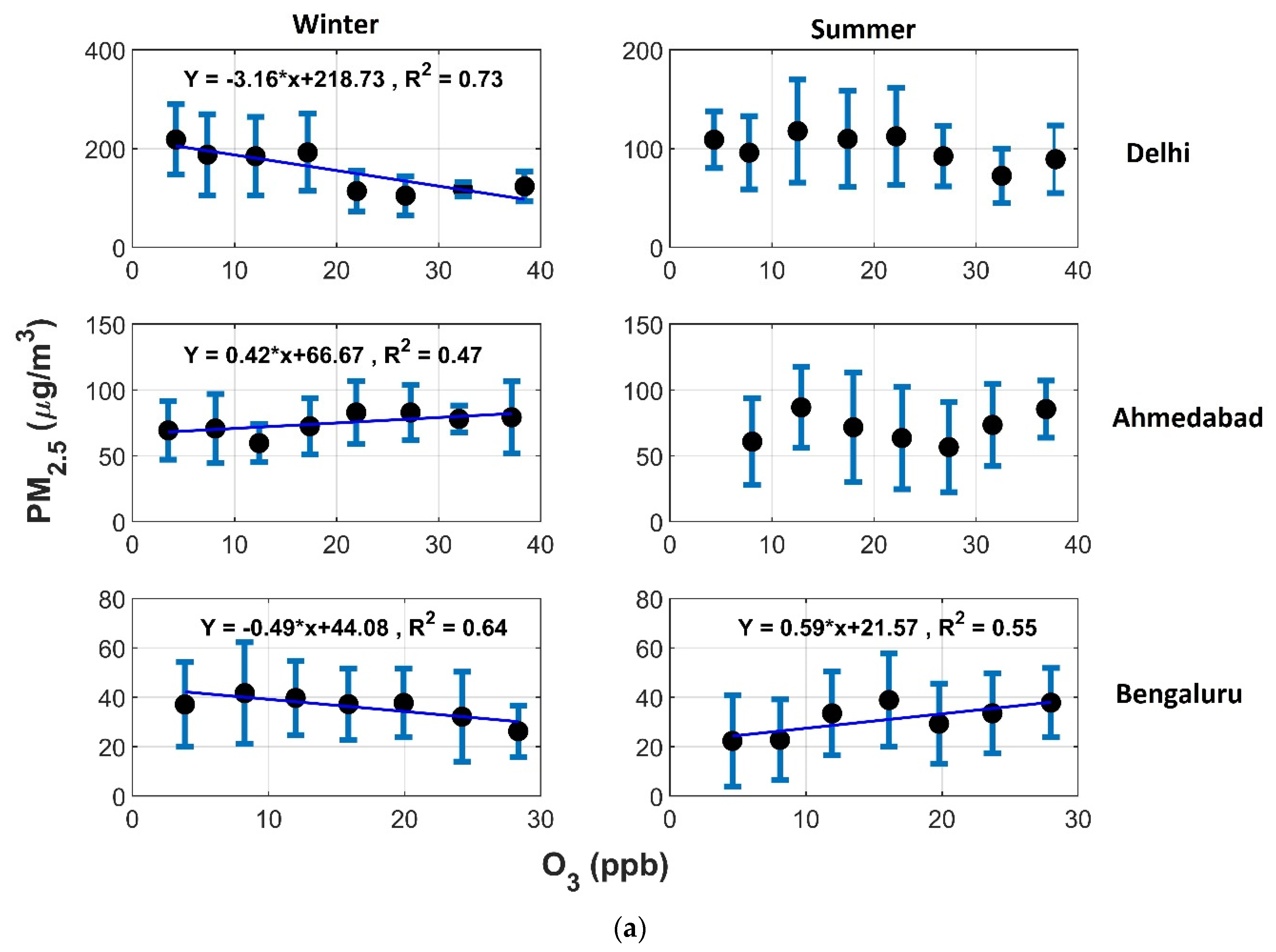
Figure 4a shows the overall relationship between PM2.5 and O3 during the summer and winter seasons for all three selected locations. It was observed that there is no significant correlation between PM2.5 and O3 during the summer season in both Delhi and Ahmedabad. Ahmedabad is a dust-dominated area, and Delhi has very high local emissions; hence, SOAs would only be a small fraction of the atmosphere of these cities during summer. Bengaluru shows a positive relation between PM2.5 and O3 during the summer with R2 = 0.55, which is significant at the 90% confidence level (p = 0.0577). Due to maximum insolation during the summer in Bengaluru, the increase in O3 concentration due to photochemical reactions may also increase the oxidative capacity of the atmosphere, thus encouraging the formation of SOAs.
During winter, Delhi experiences high PM pollution and reduced solar radiation due to foggy and hazy conditions. These conditions restrict O3 formation and also reduce SOA formation. Additionally, the lower boundary layer height during winter increases aerosol loading, and O3 formation is reduced due to fewer sunshine hours. Therefore, during the winter season, the relationship between PM2.5 and O3 in Delhi and Bengaluru is negative, with R-squared values of 0.73 and 0.64, respectively. This negative relationship for Delhi and Bengaluru is significant at 99% (p = 0.0072) and 95% (p = 0.031) confidence levels, respectively. Ahmedabad, however, shows a positive relation between PM2.5 and O3 during winter, where R2 = 0.47 is significant at the 90% confidence level (p = 0.0606)). The negative correlation between PM2.5 and O3 over Delhi in winter points to the combined impact of physical O3 destruction and the inhibition of photochemical production.
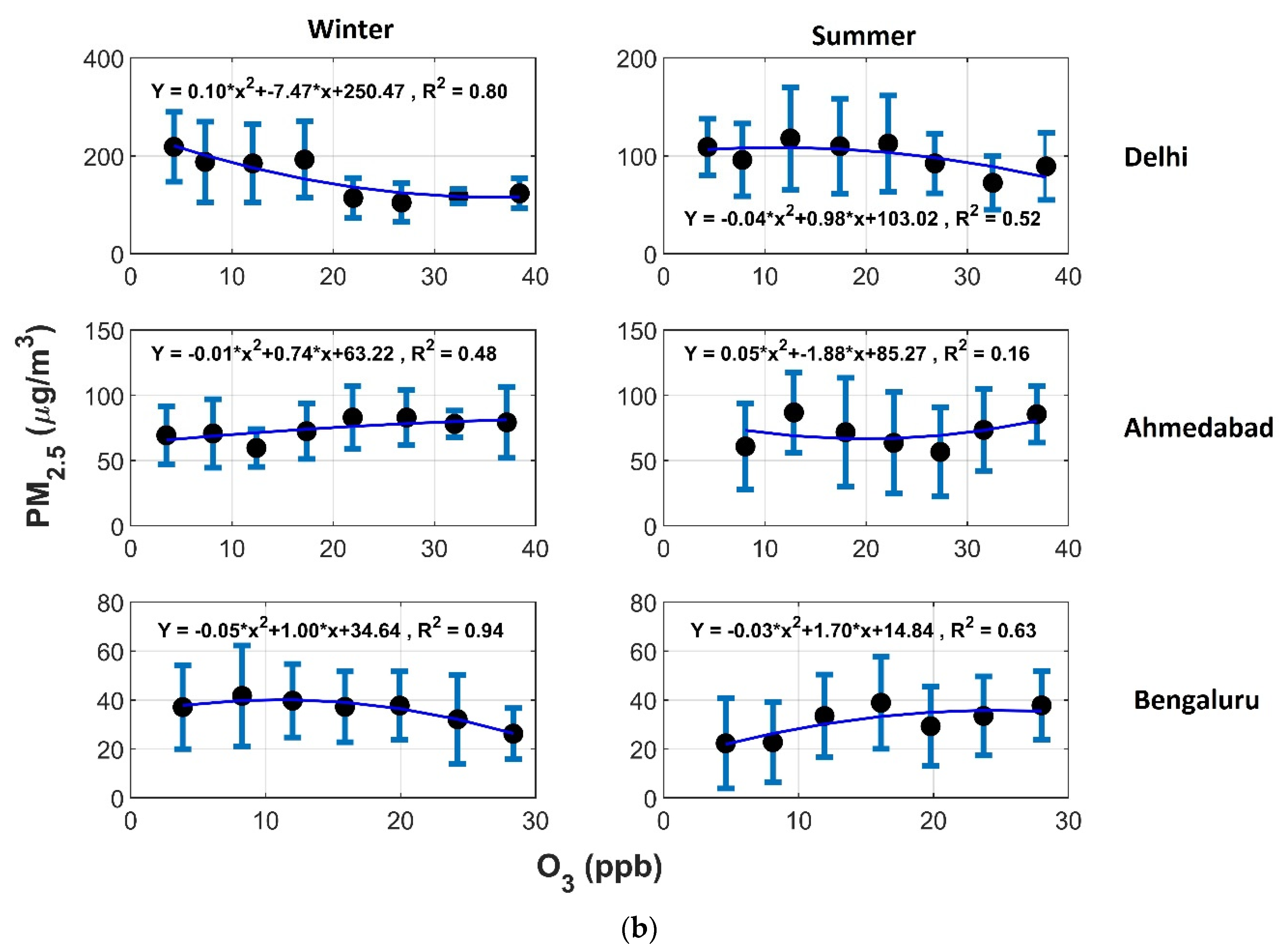
During the summer months in Delhi, no significant correlation was observed (Figure 4a), but when a regression analysis of second order was performed between PM2.5 and O3 (Figure 4b), a positive correlation was observed, with R2 = 0.52. The negative quadratic term explains that the nonlinear increase in PM2.5 concentrations with O3 is less than the linear increase. Additionally, the quadratic curve fits better for the regression of summer months in Bengaluru, with an improved R2 of 0.63. The negative quadratic term here shows that the linear increase dominates the nonlinear increase; therefore, the increase in PM2.5, with increasing O3 concentrations, is less than linear. However, Delhi during winter shows a negative correlation, but the quadratic term is positive here, which explains that the nonlinear relationship between PM2.5 and O3 dominates over the linear relationship. For Ahmedabad during winter, not much change in R2 is seen for both linear and quadratic regression, but the negative quadratic term in the quadratic regression explains that the increase in PM2.5 with increasing O3 is less than linear. Additionally, the quadratic curve fits better, with improved R2 (0.94), for Bengaluru during winters. In short, the dependence of PM2.5 and O3 on each other is not fully linear and consists of some nonlinear relationships due to additional dependencies, which need to be explored.
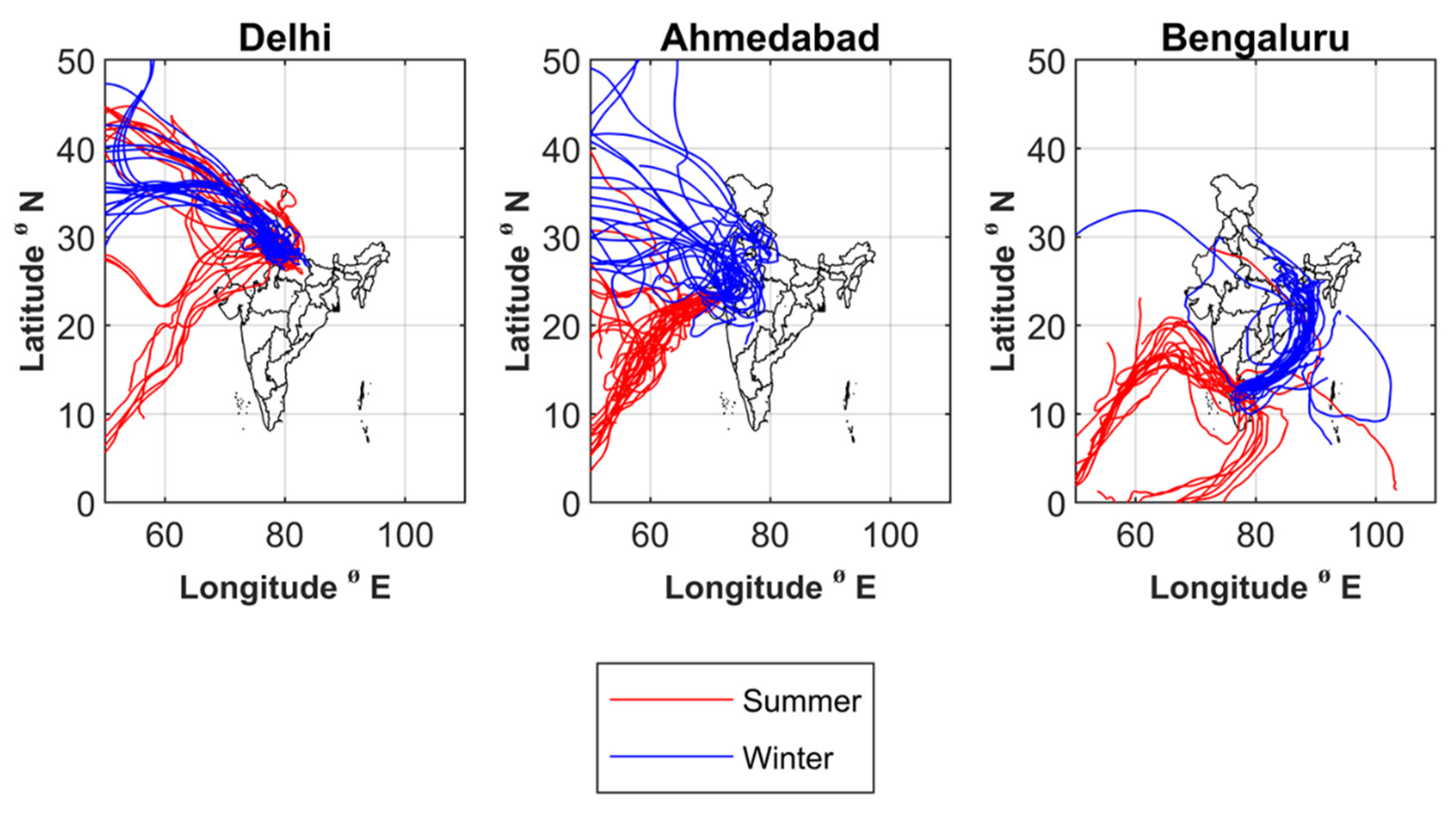
The fate of reactive pollutants can be significantly influenced by wind-borne transport (wind speed and wind direction) by low-level prevailing winds [42,43]. The HYSPLIT trajectories at 300 m above ground level are shown in Figure 5 (https://www.ready.noaa.gov/HYSPLIT.php, accessed on 20 March 2021). The three plots show 10-day backward trajectories at the three selected cities, Delhi, Ahmedabad and Bengaluru, for the year 2020. Winds in Delhi and Ahmedabad during summer originate from the southwest region. Dust storms, occurring every year between March and June in the summer months, represent one of the primary pollutant sources originating from the Arabian Peninsula and the Thar Desert in northwestern India [44]. In summer, Bengaluru is influenced by long-range transportation from the Arabian Sea as well as the north Indian Ocean, which brings lots of humidity to the region. During winter, the backward trajectory shows that air masses from the western part of India and the bordering Pakistan region can influence the level of pollutants in Ahmedabad and Delhi, while Bengaluru is influenced by the air masses mostly from the IGP, eastern India and the Bay of Bengal.
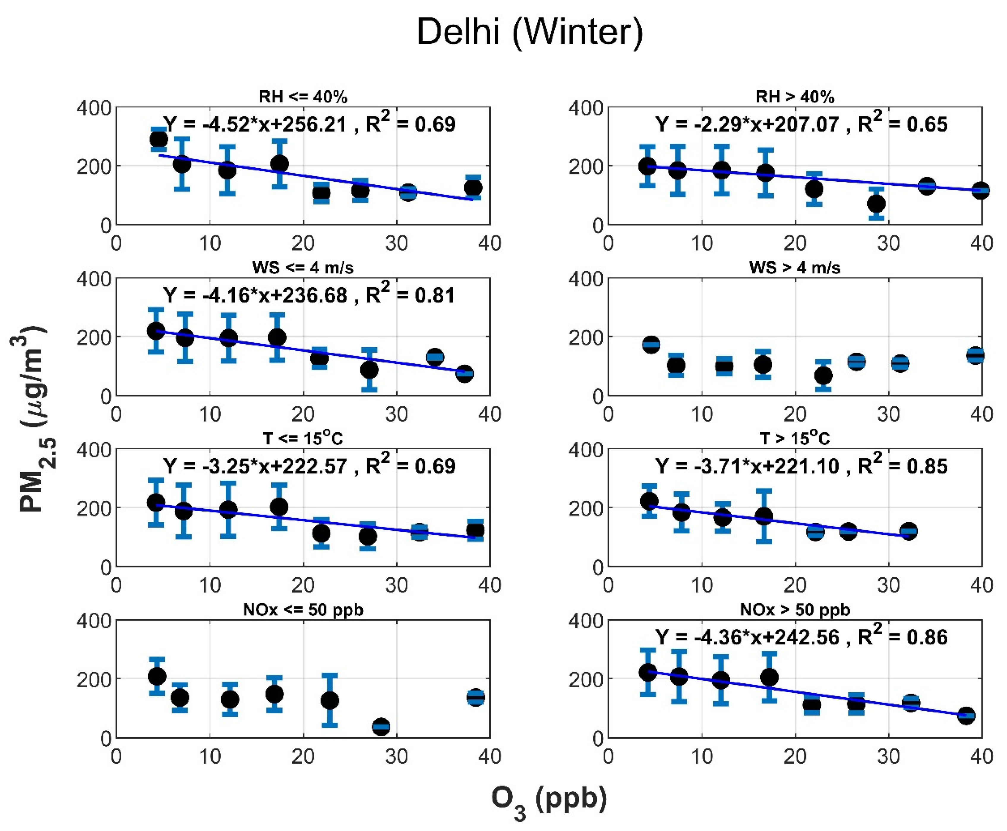
3.1. Dependence of PM2.5 on O3 for Different Meteorological and Chemical Parameters in Delhi during Winter and Summer
Figure 6 shows the relation between PM2.5 and O3 in Delhi during the winter season. The regression between PM2.5 and O3 was observed for different ranges of meteorological parameters, viz., RH, WS and T. Delhi experiences very high levels of aerosol concentration during winters due to high particulate pollution. Throughout wintertime, the meteorological conditions over Delhi and other parts of the IGP are represented by low boundary layer height, calm winds, frequent temperature inversions, and high RH [45]. Ram et al. (2010) [46] explained that these conditions favour the accumulation of aerosols and also the formation of SOAs. At the same time, calm and stable conditions with high PM2.5 favour the dry depositional loss of O3.
Delhi experiences severe foggy conditions during winter. Tiwari et al. (2011) [47] studied the influence of increased aerosol content on fog formation during winters in Delhi. Due to high aerosol content and hazy conditions, the amount of incoming solar radiation is decreased. The relationship between PM2.5 and O3 during wintertime is negative for both RH ≤ 40% and RH > 40% (significant at the 95% confidence level, p = 0.010 for RH ≤ 40% and p = 0.015 for RH > 40%). Irrespective of the RH levels, the R2 between PM2.5 and O3 does not show much difference, but the increase of the slope from −4.52 for RH ≤ 40% to −2.29 for RH > 40% indicates that the negative relationship weakens when the RH increases in Delhi. Hence, it can be said that the increased RH favours aqueous chemistry and the formation of new particles. A strong negative relationship, with R2 = 0.81 (p = 0.0025), is observed for WS ≤ 4 m/s. However, when WS increases, i.e., when WS > 4 m/s, no significant relation is observed. For all temperature ranges, the PM2.5 and O3 levels show a significant negative relationship, R2 = 0.69 for T ≤ 15 °C (significant at the 95% confidence level, p = 0.010) and R2 = 0.85 for T > 15 °C (significant at the 99.9% confidence level, p = 0.0029).
Hama et al. (2020) [48] reported that the O3 concentration is lower during the winter months in Delhi and stated that it is because of meteorological conditions and secondary chemical factors such as variations in NOx and VOC. Guo et al. (2017) [49] explained that the low levels of O3 in winter may be because of lower solar radiation and fewer sunshine hours. Hama et al. (2020) [48] also found that NOx levels in Delhi showed the highest levels during winter. For NOx > 50 ppb, a strong negative relationship is observed with R2 = 0.86, which is significant at the 99.9% confidence level (p = 0.0009). However, for NOx < 50 ppb, no significant correlation is seen.
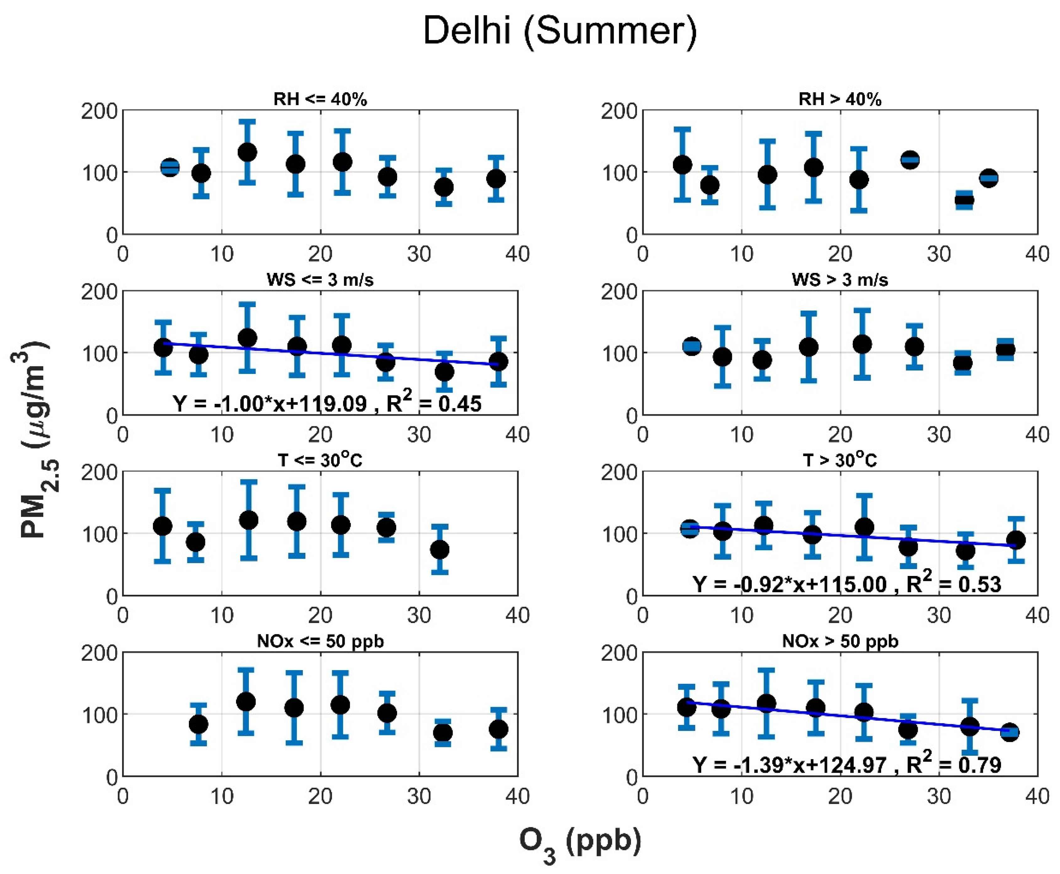
Figure 7 shows the relation between PM2.5 and O3 during the summer season in Delhi. Delhi experiences a very high temperature, with increased boundary layer height and higher WS, during the summer seasons. The maximum temperature during summer in Delhi is 45 ± 3 °C [50]. Thus, the emissions are diluted into a deeper atmospheric boundary layer. Therefore, a negative relationship between PM2.5 and O3 is observed for T > 30 °C, with R2 = 0.53 (significant at the 95% confidence level, p = 0.040). The ventilation effect also comes into play and lowers the pollution in Delhi. Hama et al. (2020) [12] observed that the O3 concentration starts increasing in the summer seasons. Higher temperatures and solar radiation enhance the photochemical oxidation of precursors, leading to a higher concentration of O3 during summer [50].
The PM2.5 concentration decreases due to the ventilation effect, but there is an increase in O3 concentration due to atmospheric oxidation. Hence, we observed a negative relationship between PM2.5 and O3 during summer in Delhi due to lower WS and higher temperatures. Additionally, the HYSPLIT trajectory (Figure 5) over Delhi shows that during summertime, the winds come from the southwest, which can transport dust particles from the desert region in Rajasthan, increasing the particle concentration in the region. The dominance of natural dust in total PM2.5 loading over the anthropogenic precursors may reduce SOA yield. As primary particles will be overwhelmingly larger compared to SOAs, the increase in aerosol content due to SOA formation will not dominate in summer over Delhi. Figure 1 shows that 99% of particles over Delhi are primary emissions. Additionally, the prevailing wind speeds are higher, providing less scope for SOA formation by the accumulation of precursors. PM2.5 and O3 in Delhi are less interdependent, and their production/loss processes are governed by independent factors. In the case of O3, it is more due to photochemistry, while in the case of PM2.5, it is more due to the atmospheric transport of desert dust as well as local emissions.
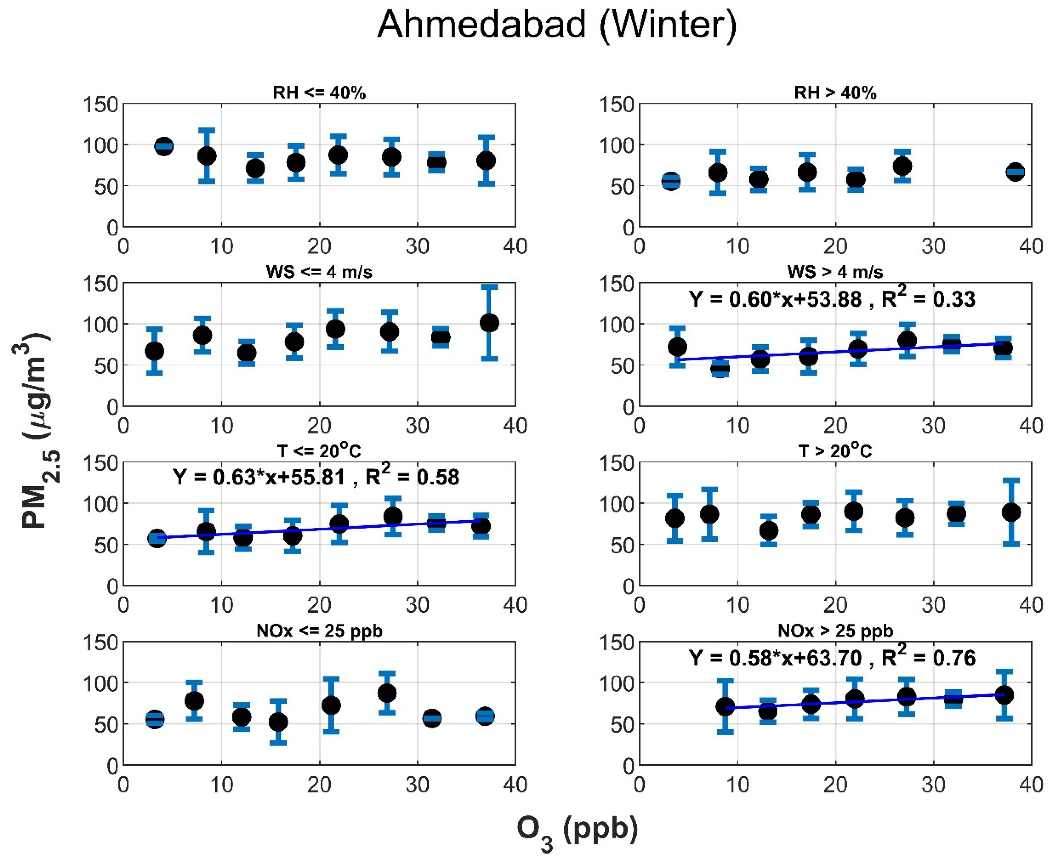
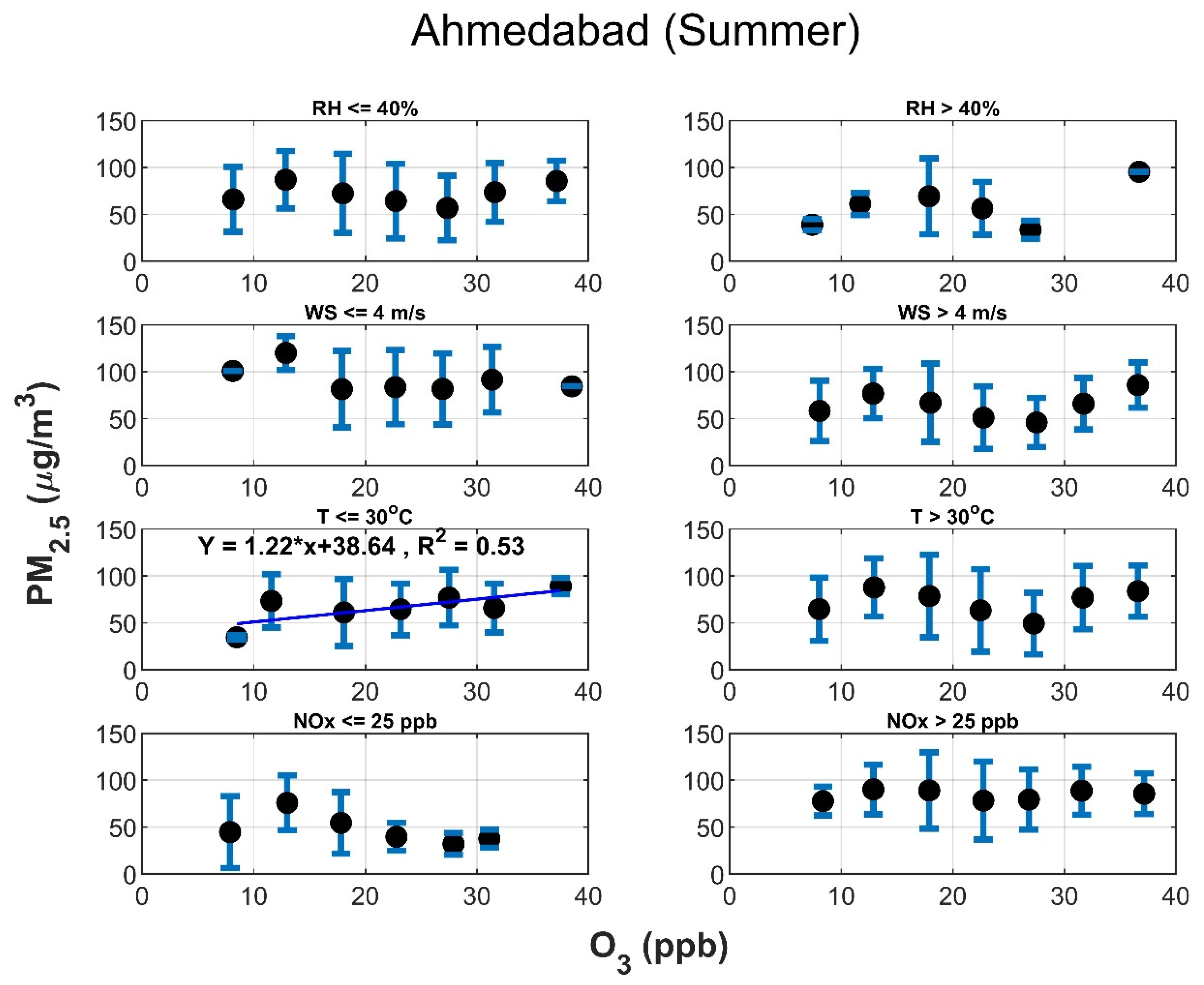
3.2. Dependence of PM2.5 on O3 for Different Meteorological and Chemical Parameters in Ahmedabad during Winter and Summer
Lal et al. (2000) [51] observed that due to increased levels of precursor gases, O3 concentrations are the greatest in the fall and winter months in Ahmedabad. The massive transports from land masses and lower boundary layer heights are the most important causes for the increase in precursor levels during the pre-winter and winter months. Additionally, wind pattern change over the Indian landmass takes place in the autumn; it turns out to be northeasterly during the pre-winter months [51]. The wind flow from the northeast leads the air towards Ahmedabad, which is rich in air pollutants and increases the levels of O3 and its precursor gases [52]. In winter seasons, like O3, NOx also attains higher levels as local emissions are confined in shallower boundaries. Therefore, NOx levels become sufficiently high during winter to create O3 during the daytime.
Additionally, in cold weather, the pollutants from different sources get trapped in the boundary layer by frequent temperature inversions. In this manner, the concentration of PM2.5 is typically higher during cold weather months. NO2 is the only chemical source of tropospheric O3, and because of higher NOx concentrations in the atmosphere during the winter months, the production of O3 is favoured. Hence, a positive relationship is observed between PM2.5 and O3 for higher NOx, with R2 = 0.76, significant at the 95% confidence level (p = 0.010) (Figure 8). Higher O3 can increase oxidation capacity and recycling efficiency, leading to higher OH, and SOA formation can be favoured, leading to an increase in PM2.5. A positive relationship can be seen for temperatures below 20 oC (R2 = 0.58, p = 0.0281). This dependence is significant at the 95% confidence level. Rengarajan et al. (2011) [53] studied aerosol acidity during wintertime in Ahmedabad and found that the enhancement of SOA formation during winter in Ahmedabad was favoured due to the high level of aerosol acidity.
Figure 9 shows the relation between PM2.5 and O3 in Ahmedabad during the summer season. The meteorological conditions in Ahmedabad favour the production of O3 from photochemical reactions [54]. However, in Ahmedabad, being a dust-dominated area, the oxidative capacity of the atmosphere can be considerably reduced due to HO2 uptake by dust affecting the SOA formation [55,56]. Sudheer et al. (2015) [57] studied the role of RH in SOA formation in Ahmedabad and observed a negative correlation between atmospheric water vapour and secondary organic carbon in PM2.5 and PM10. The authors explained that the possible reasons could be either the local wind bringing air masses with higher atmospheric water vapour and low VOCs or the variation of oxidising species such as OH radicals in the ambient atmosphere. The PM2.5 concentration is also reduced during summer due to higher PBL, leading to a dilution effect [10]. No significant correlation is observed between PM2.5 and O3 during the summer season (Figure (9)).
3.3. Dependence of PM2.5 on Ozone for Different Meteorological and Chemical Parameters in Bengaluru during Winter and Summer
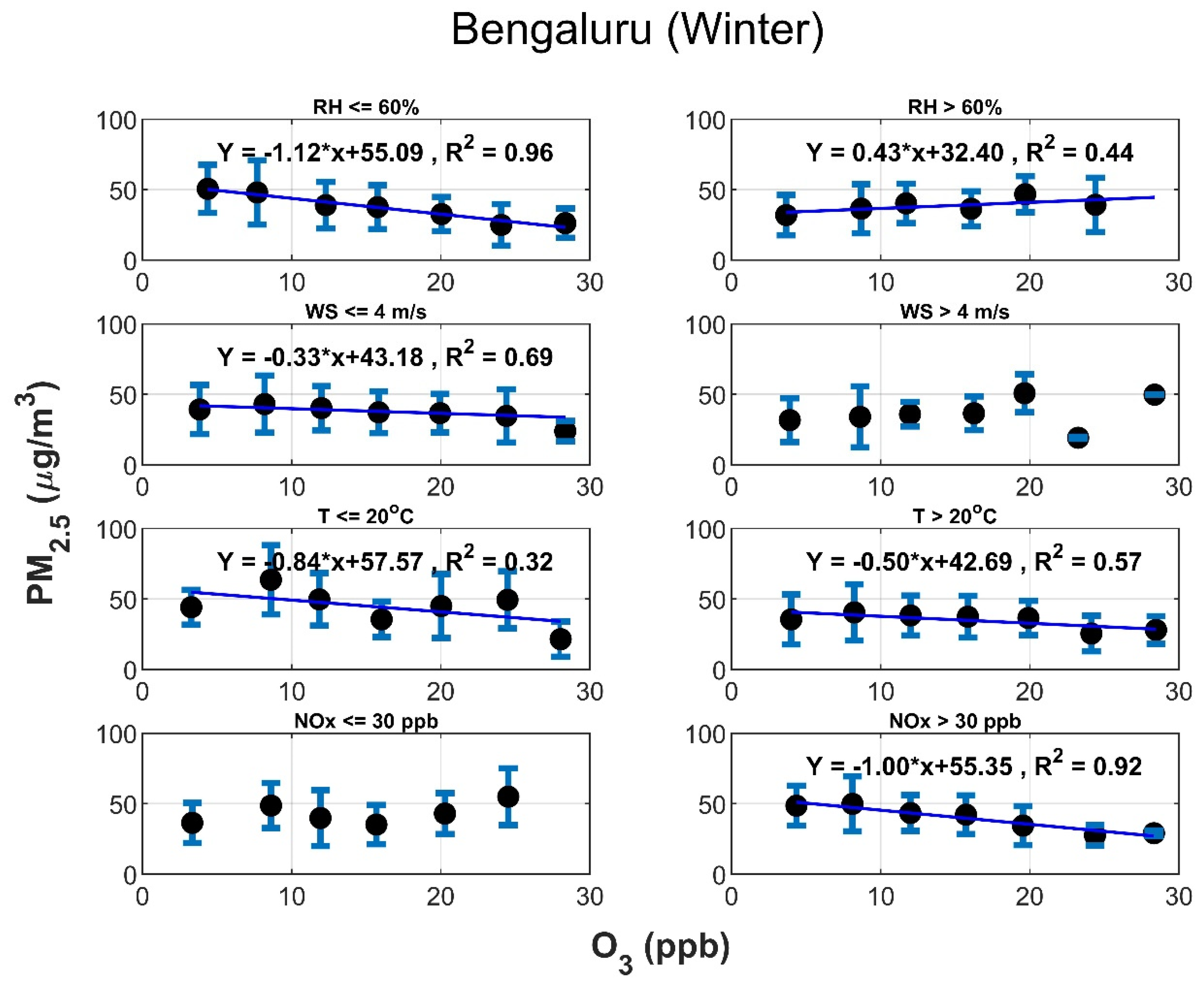
Figure 10 shows the relation between PM2.5 and O3 for Bengaluru during wintertime. During the winter, the aerosol concentration increases due to emissions accumulating in a lower PBL, and due to this, there is a reduction in the incoming solar radiation. Thus, O3 formation due to photochemical reaction is reduced. Therefore, during the winter, a negative correlation between PM2.5 and O3 is observed. The R-squared is 0.96 for RH below 60% (p = 0.0001), 0.92 for NOx > 30 ppb (p = 0.00054), 0.57 for T > 30 oC (p = 0.049) and 0.69 for WS < 4 m/s (p = 0.020). The dependence is significant at the 99.9% confidence level for RH below 60% and for NOx > 30 ppb. Additionally, for T > 30 oC and for WS < 4 m/s, the dependence is significant at the 95% confidence level. Thus, calm wind, less humidity, and high NOx conditions result in an inverse relationship between PM2.5 and O3. These conditions lead to less O3 production and promote O3 destruction (physical as well as chemical) on one hand, while favouring new particle formation and accumulation on the other hand. However, for WS > 4 m/s, no significant correlation could be found. This is due to the ventilation effect; the PM2.5 concentration reduces because of dilution due to wind conditions.
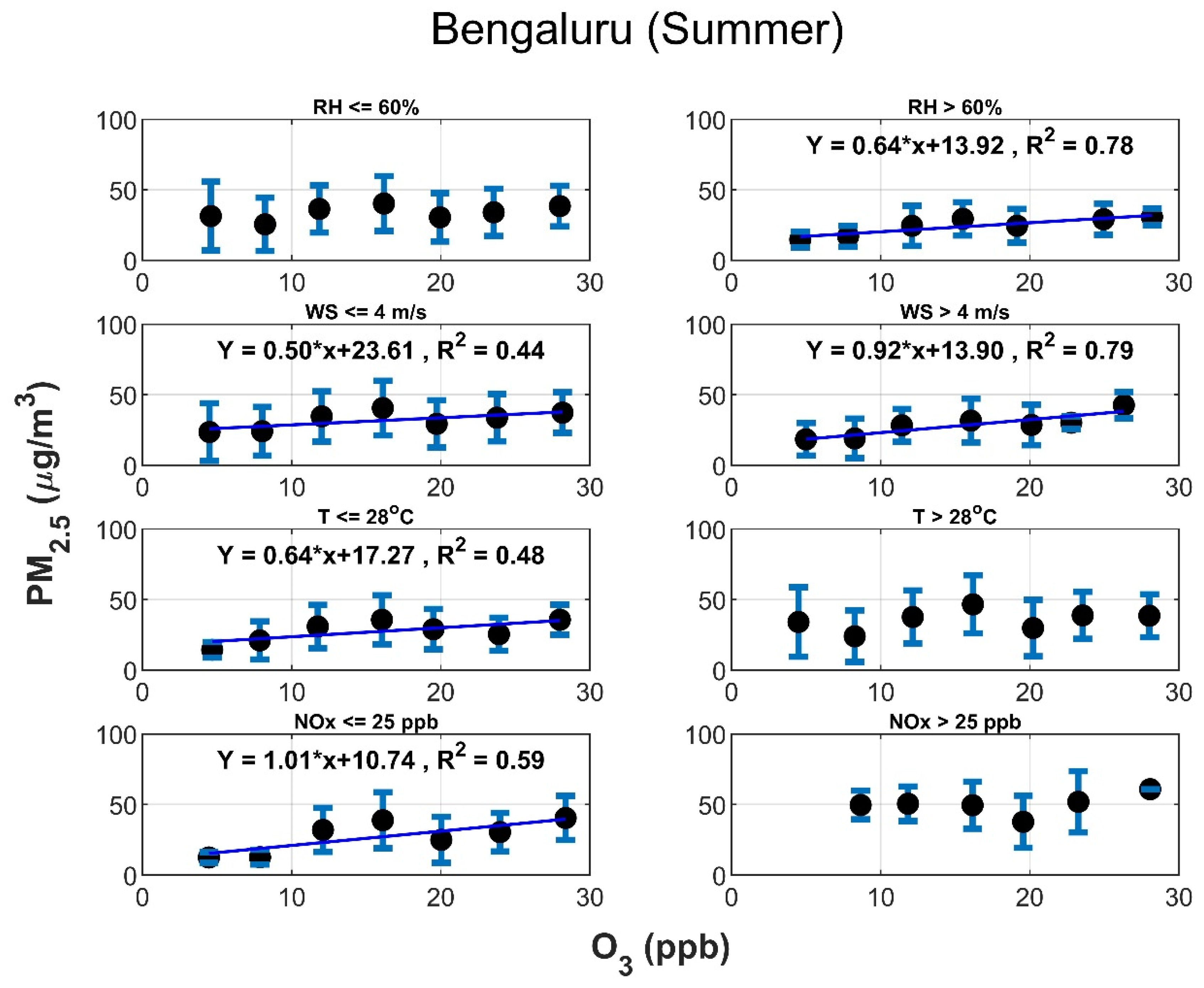
Figure 11 shows the relation between PM2.5 and O3 during summertime in Bengaluru. The R-squared is 0.78 for RH > 60% (p = 0.0083), 0.79 for WS > 4 m/s (p = 0.007) and 0.59 for NOx < 25 ppb (p = 0.045), and this relation is significant at the 99% confidence level for RH > 60% and WS > 4 m/s and the 95% confidence level for NOx < 25 ppb. Thus, a humid, ventilated, low NOx atmosphere is conducive to a positive relationship between O3 and PM2.5. Ventilated conditions allow NOx levels to be below titration limits, favouring O3 build-up, while increased RH and oxidant levels promote new particle formation. Higher wind speed supports the optimum moisture levels from oceanic air masses. O3 production is enhanced during summertime due to longer day hours and maximum insolation. This positive relation between PM2.5 and O3 in summer can be strengthened by the increased lifetime of oxidants in the atmosphere that reacts with the organic gases and forms SOAs [58]. Additionally, the effect of the transport of pollutants can also be seen during summertime in Bengaluru as the R2 increases from 0.44 for WS < 4 m/s to 0.79 for WS > 4 m/s.
3.4. Role of Atmospheric Transport Inferred from FLEXPART
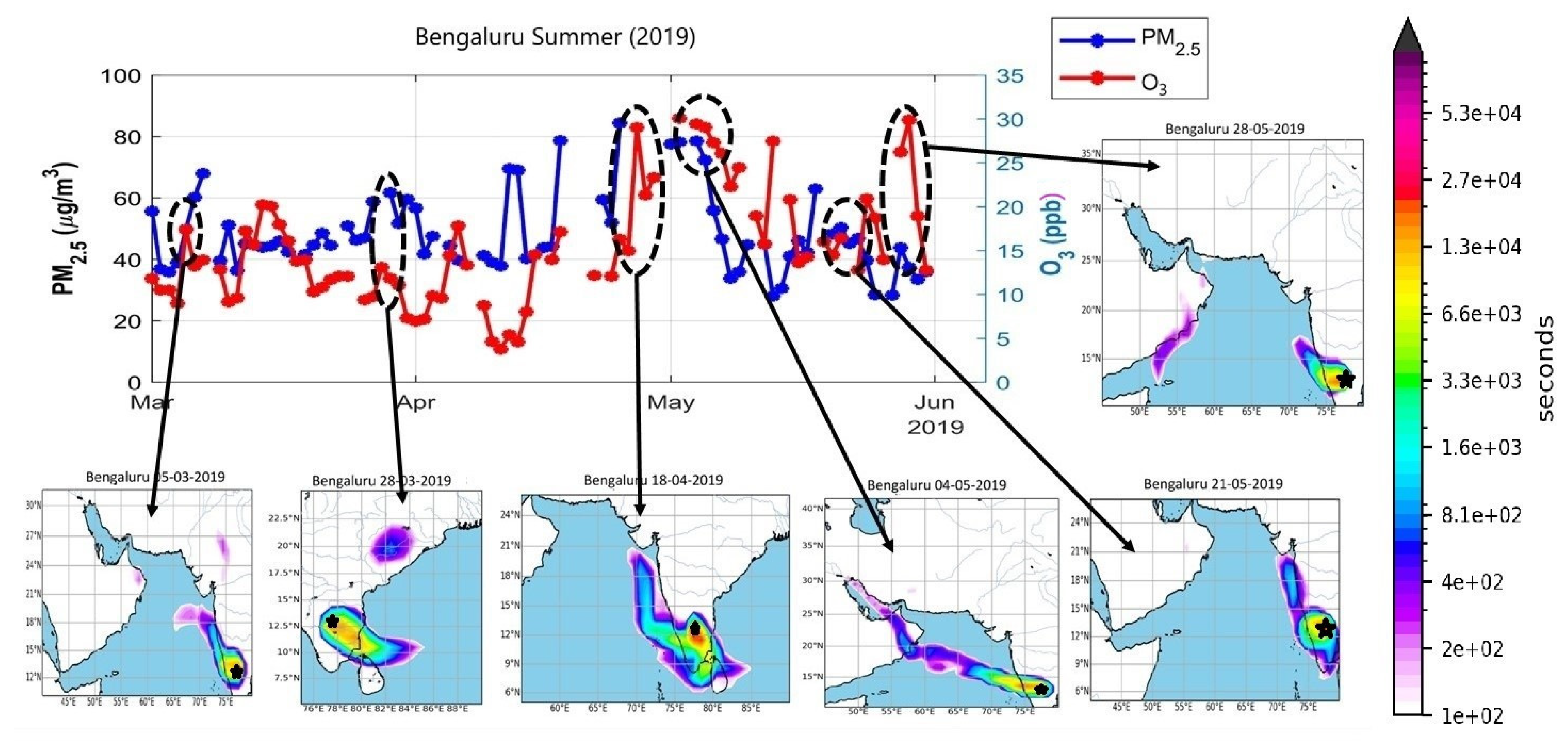
The positive correlation between PM2.5 and O3 in summer over Bengaluru creates an important prospect to analyse the interdependence of SOA formation through the presence of atmospheric oxidants under various meteorological regimes. Figure 12 shows the backward trajectory of FLEXPART for the 2019 summer days in Bengaluru. Some days saw a rise in both PM2.5 and O3 concentrations; the air mass backward trajectory is displayed for those days (encircled points in Figure 12). The RH was quite low (below the 25th percentile) during the first few weeks of summer 2019, and the air mass trajectory revealed that winds were predominantly from the Bay of Bengal. In addition, the wind speed throughout that time period was between 3 and 4 m/s. However, no significant relationship between O3 and PM2.5 was observed in these air masses. The air masses came predominantly from the Arabian Sea side in the later part of the summer of 2019. The RH was above the 75th percentile on the days when both PM2.5 and O3 levels increased at the same time. Furthermore, when the air masses arrived from the Arabian Sea, the wind speed was below the 25th percentile (<3 m/s). The slower wind speed and high RH offered favourable conditions for the production of SOAs in Bengaluru during the summer days of 2019. FLEXPART images (e.g., on 28 May 2019) clearly show the greater influence of close-by regions due to slow winds, leading to enhancements in PM2.5. The rise in PM2.5 concentrations with the increase in O3 is likely due to the formation of SOAs in moist air masses. Further, during periods of convergence of air masses from the Arabian Sea and the Bay of Bengal, a sharp enhancement was observed in both O3 and PM2.5 (e.g., 18 April 2019). The PBL height in March, April and May of 2019 was 2511, 2686, and 2125 m, respectively. In March, April and May, the PM2.5 concentrations were 48.0, 52.3, and 46.6 µg/m3, respectively. The PBL height rose by 7% in April compared to March, while the PM2.5 concentration increased by 9%. Normally, particle concentrations fall as PBL height increases; however, in this case, the PM2.5 concentration increases. Additionally, Prabhu et al. (2022) [59] observed an overall weak positive correlation between O3 and PM2.5 on an hourly and daily basis in Bengaluru, where a 1 µg/m3 increase in hourly PM2.5 was associated with an increase of ~ 0.2 ppb of hourly O3, while a 1 µg/m3 increase in daily PM2.5 was associated with an increase of ~ 0.6 ppb of daily O3. This clearly indicates the role of secondary chemistry.
From the above observations, it is understood that Bengaluru and Delhi behave in completely opposite ways when it comes to secondary chemistry. The formation of secondary particles is significantly impacted by the local climate and prevailing meteorological conditions in these places. Additionally, the effect of RH in different emission regimes on SOA formation is different, and it needs to be studied for a better understanding of secondary chemistry.
3.5. Predicting the Ozone Concentration Using Recurrent Neural Networks (RNNs)
The above analysis shows that the concentration of O3 for a particular region depends on different meteorological and chemical parameters, such as PM2.5, WS, T, RH and NOx. Furthermore, the production of SOAs due to oxidation during the summer months is the link between aerosols and O3. The observed dependencies are not always linear, as evinced by Figure 4b. Despite PM and O3 posing serious threats to the Earth’s climate and human health at elevated levels [60], there are no long-term measurements of atmospheric pollutants in several places of significant urban populace. It is, therefore, of great importance to conduct studies to fill this gap, as chemistry–climate models have a tendency to reproduce already scarce measurements but with a considerable bias. The uncertainties surrounding emission inventories and the parameterizations of physical and chemical processes also contribute to the biases present in these models. In addition to these biases, conventional models also require significant computing resources, which can be a limiting factor in conducting high-resolution simulations [61]. Artificial intelligence (AI) and machine learning (ML) have emerged as powerful alternative tools for modelling in various fields, including Earth system science. The use of ML in climate modelling is an active area of research and has the potential to improve our understanding of the climate system and enable more accurate projections of future climate change. Particularly, due to very complex chemistry involving NOx and multiple hydrocarbons through a plethora of photochemical reactions, reliable predictions of surface O3, specifically over the Indian region, have still eluded the atmospheric modelling community. While the first part of this study has elucidated the various important meteorological and photochemical dependencies of surface O3, the possibilities of using these observed dependencies for the prediction of O3 create an interesting prospect that needs to be tested. Therefore, an attempt is made to predict the value of O3 if other factors are known through artificial intelligence. Here, Recurrent Neural Network models (RNNs) predict the O3 concentrations for the summer seasons of 2019 and 2020 using the parameters mentioned above.
3.5.1. Experimental Setting
The experiment runs on an Ubuntu 18.04 Linux system with 16 GB of RAM, an Intel(R) Core (TM) i7-8700 CPU running at 3.20 GHz, and RX RADEON Graphics Cards (4 GB). Python 3.7 with Pandas, Numpy, Tensorflow, and Keras is used for data processing and modelling. For reducing the errors between prediction and observation, we use mean squared error (MSE) as the loss function and optimiser; 70% of the dataset was utilised for training, and 30% was used for validation in this study. The model’s performance in the validation set determines the hyper-parameters. For successful learning, the Early Stopping method is used, in which a training process can be halted when the validation loss stops reducing. Multiple approaches are used to assess the statistical significance of model findings and discover differences between groups to undertake rigorous statistical analysis. Several statistical indices are used to evaluate the effectiveness of the suggested model, including the mean absolute error (MAE), the root mean square error (RMSE), and the coefficient of determination (R2).
3.5.2. Experimental Results
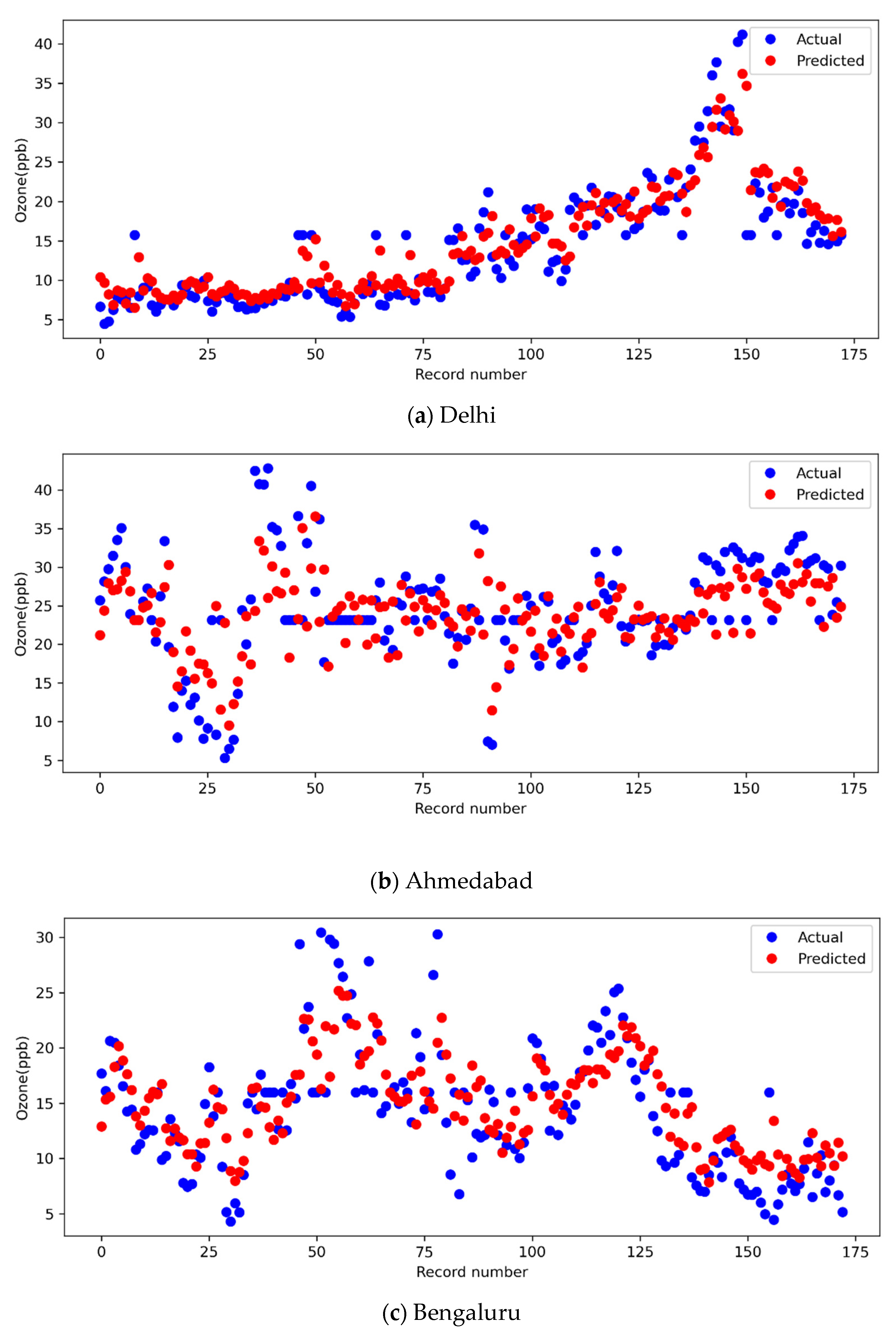
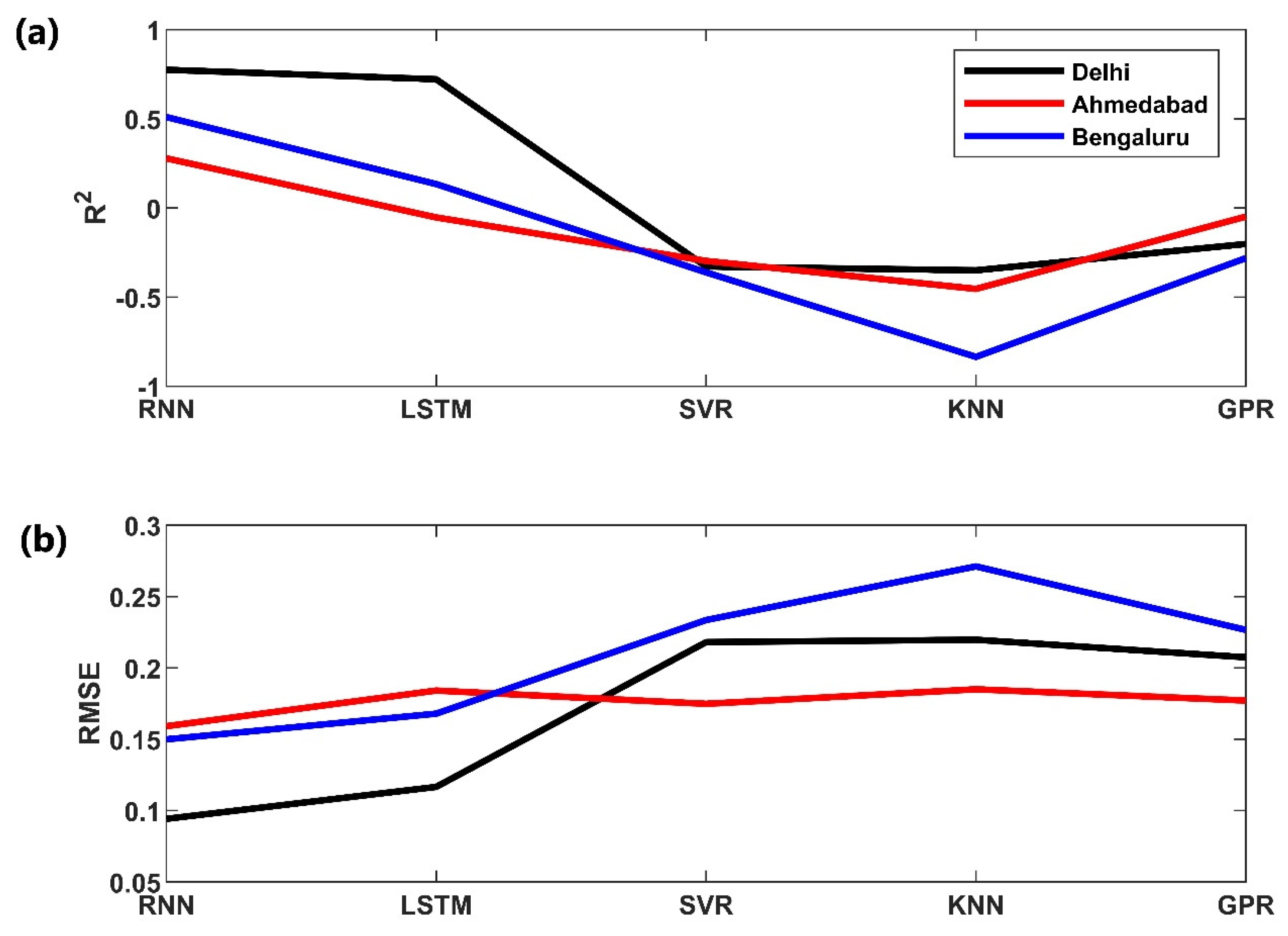
To assess the proposed RNN deep learning model’s efficiency, we contrasted the experimental results with other machine learning techniques, such as LSTM (Long Short-Term Memory), KNN (K- Nearest Neighbor), SVR (Support Vector Regression), and GBR (Gradient Boosted Regression). The LSTM model is an advanced RNN that is capable of handling long-term dependencies and allowing information to persist [62]. KNN is a machine learning algorithm that classifies the data based on its similarities and places the new data in the category that matches the existing categories the closest [63]. SVR is a regression algorithm that supports both linear and nonlinear regressions, and it is used for predicting continuous ordered variables by fitting the error inside a certain threshold instead of minimising the error, which is the case in simple regression [64]. GBR is a machine learning algorithm in which each predictor corrects its predecessor’s error [65]. Figure 13 shows the prediction of O3 levels using RNN model during summer season over the three study locations. The comparison of model performance can be found in Table 3 and Figure 14.
The results indicate that an RNN’s primary method may efficiently learn the many dynamic time scales present in the complex data. RNNs exhibit a high degree of generalisation for patterns not covered in the training phase. Other techniques attempted here are sensitive to hidden neurons and have poor generalisation for new inputs due to the over-training problem. These networks’ topological features enable them to analyse temporal data. These networks also can reproduce nonlinear input–output mappings, thanks to intrinsic nonlinear components and sets of trainable weights. Between the output of the hidden layer and the input of the RNN, there is a time-delayed feedback loop. This loop supplies memory to the network, enhancing its capacity to describe dynamical systems significantly.
4. Summary and Conclusions
The present study focuses on finding the relationship between PM2.5 and O3 in different Indian cities during the summer and winter seasons. The locations were selected based on long-term data availability, and the selected stations also represent contrasting climatic conditions and varied emission, meteorological and air mass regimes. The sources of PM2.5 were identified for all the selected stations. To find the relation between PM2.5 and O3, regression analysis was performed during the winter and summer seasons for different ranges of meteorological variables. It was found that the negative correlation in Delhi during winter is due to the lower photochemical production of O3 as the incoming solar radiation is reduced due to higher PM2.5 concentrations. The ventilation effect plays a major role in the negative correlation between PM2.5 and O3 during the summer in Delhi. A positive relation between O3 and PM2.5 was observed for higher WS during winter in Ahmedabad due to transport from polluted areas. No significant correlation was observed between PM2.5 and O3 during summer in both Delhi and Ahmedabad due to the high background of primary particles, dominated by dust from the Arabian Peninsula during summer. Thus, the effect of O3 on SOA formation becomes obscured, and no significant relationship can be traced between PM2.5 and O3 during summer. Bengaluru shows a positive correlation during summer, indicating the formation of SOA. Due to higher PM2.5 concentration and lesser insolation, O3 production is reduced in Bengaluru during winter; hence, a negative relationship is observed between PM2.5 and O3 during winter. However, there is very clear evidence for SOA formation during enhanced O3 periods, promoted by humid marine air masses, mainly from travelling at low speed over to Bengaluru in summer. The simultaneous enhancements in O3 and PM2.5 were more frequent when the air masses came from the Arabian Sea side compared to the Bay of Bengal side. The dependencies for O3 observed in this study are redirected towards the prediction of this very important atmospheric chemical parameter through the use of Recurrent Neural Network models (RNNs) as it poses a global threat to human health, ecosystems and climate. The results indicated that RNNs are capable of effectively learning complex, dynamic data and have strong generalisation capabilities and can be potentially useful to fill up gaps in the prediction of O3. In contrast, other techniques struggle with generalising to new inputs due to over-training and their sensitivity to hidden neurons. RNNs were able to analyse temporal data and model nonlinear input–output relationships due to their topological features and nonlinear components. The addition of a time-delayed feedback loop between the hidden layer and the input of the RNN enhanced the network’s ability to describe dynamic systems. This study is an important step in understanding the relationships between O3 and PM2.5 with regard to different meteorological conditions and SOA formation. The dependency analysed in this study will provide important insight for design strategies for air quality management in urban regions.
Supplementary Materials
The following supporting information can be downloaded at: https://www.mdpi.com/article/10.3390/urbansci7010009/s1. O3-PM-relation.xlsx contains the main data used in this study.
Author Contributions
K.K.M. and S.K. developed the neural-network-based predictions. H.G. and A.A. conducted FLEXPART simulations. R.K.Y., S.L. and C.M. conducted the data analysis and MS writing. CM conceptualized the study. All authors have read and agreed to the published version of the manuscript.
Funding
This research was funded by DST-SERB-SRG (Grant No: SRG/2020/001006) and ISRO-GBP-ATCTM for research equipment and salary of first author. We thank the editor of URBAN Science for kindly waiving off the APC for this article. We also thank the editor and the two anonymous reviewers for getting the MS much improved through their reviews and comments.
Institutional Review Board Statement
Not applicable.
Informed Consent Statement
Not applicable.
Data Availability Statement
The data presented in this study are available in the Supplementary data file (O3-PM-relation.xlsx).
Acknowledgments
The air quality data were downloaded from the CPCB website: https://app.cpcbccr.com/ccr/#/caaqm-dashboard/caaqm-landing/caaqm-comparison-data, accessed on 10 March 2021. The PM2.5 sources are based on the analysis presented in URBAN emissions.info. The meteorological data were obtained from NASA/POWER. PBL data were obtained through HYSPLIT simulations. S.L. thanks INSA, New Delhi, for the position and the Director, PRL, Ahmedabad, for the support. C.M. thanks DST-SERB-SRG (SRG/2020/001006) and ISRO-GBP-ATCTM for the support received.
Conflicts of Interest
The authors declare no conflict of interest.
References
- Xing, J.; Wang, S.; Zhao, B.; Wu, W.; Ding, D.; Jang, C.; Zhu, Y.; Chang, X.; Wang, J.; Zhang, F.; et al. Quantifying Nonlinear Multiregional Contributions to Ozone and Fine Particles Using an Updated Response Surface Modeling Technique. Environ. Sci. Technol. 2017, 51, 11788–11798. [Google Scholar] [CrossRef] [PubMed]
- Benas, N.; Mourtzanou, E.; Kouvarakis, G.; Bais, A.; Mihalopoulos, N.; Vardavas, I. Surface Ozone Photolysis Rate Trends in the Eastern Mediterranean: Modeling the Effects of Aerosols and Total Column Ozone Based on Terra MODIS Data. Atmos. Environ. 2013, 74, 1–9. [Google Scholar] [CrossRef]
- Jia, M.; Zhao, T.; Cheng, X.; Gong, S.; Zhang, X.; Tang, L.; Liu, D.; Wu, X.; Wang, L.; Chen, Y. Inverse Relations of PM2.5 and O3 in Air Compound Pollution between Cold and Hot Seasons over an Urban Area of East China. Atmosphere 2017, 8, 59. [Google Scholar] [CrossRef] [Green Version]
- Meng, Z.; Dabdub, D.; Seinfeld, J.H. Chemical Coupling between Atmospheric Ozone and Particulate Matter. Science 1997, 277, 116–119. [Google Scholar] [CrossRef] [Green Version]
- Huang, R.J.; Zhang, Y.; Bozzetti, C.; Ho, K.F.; Cao, J.J.; Han, Y.; Daellenbach, K.R.; Slowik, J.G.; Platt, S.M.; Canonaco, F.; et al. High Secondary Aerosol Contribution to Particulate Pollution during Haze Events in China. Nature 2015, 514, 218–222. [Google Scholar] [CrossRef] [PubMed] [Green Version]
- Sun, Y.; Wang, Z.; Fu, P.; Jiang, Q.; Yang, T.; Li, J.; Ge, X. The Impact of Relative Humidity on Aerosol Composition and Evolution Processes during Wintertime in Beijing, China. Atmos. Environ. 2013, 77, 927–934. [Google Scholar] [CrossRef]
- Kaul, D.S.; Gupta, T.; Tripathi, S.N.; Tare, V.; Collett, J.L. Secondary Organic Aerosol: A Comparison between Foggy and Nonfoggy Days. Environ. Sci. Technol. 2011, 45, 7307–7313. [Google Scholar] [CrossRef]
- Zang, L.; Wang, Z.; Zhu, B.; Zhang, Y. Roles of Relative Humidity in Aerosol Pollution Aggravation over Central China during Wintertime. Int. J. Environ. Res. Public Health 2019, 16, 4422. [Google Scholar] [CrossRef] [Green Version]
- Pandey, S.K.; Vinoj, V. Surprising Changes in Aerosol Loading over India amid {COVID}-19 Lockdown. Aerosol Air Qual. Res. 2021, 21, 200466. [Google Scholar] [CrossRef]
- Kant, R.; Trivedi, A.; Ghadai, B.; Kumar, V.; Mallik, C. Interpreting the COVID Effect on Atmospheric Constituents over the Indian Region during the Lockdown: Chemistry, Meteorology, and Seasonality; Springer International Publishing: Cham, Switzerland, 2022; Volume 194, ISBN 0123456789. [Google Scholar]
- Odum, J.R.; Hoffmann, T.; Bowman, F.; Collins, D.; Flagan, R.C.; Seinfeld, J.H. Gas/Particle Partitioning and Secondary Organic Aerosol Yields. Environ. Sci. Technol. 1996, 30, 2580–2585. [Google Scholar] [CrossRef]
- Guo, H.; Kota, S.H.; Sahu, S.K.; Hu, J.; Ying, Q.; Gao, A.; Zhang, H. Source Apportionment of PM2.5 in North India Using Source-Oriented Air Quality Models. Environ. Pollut. 2017, 231, 426–436. [Google Scholar] [CrossRef] [PubMed]
- Behera, S.N.; Sharma, M. Reconstructing Primary and Secondary Components of PM2.5 Composition for an Urban Atmosphere. Aerosol Sci. Technol. 2010, 44, 983–992. [Google Scholar] [CrossRef] [Green Version]
- Nagar, P.K.; Singh, D.; Sharma, M.; Kumar, A.; Aneja, V.P.; George, M.P.; Agarwal, N.; Shukla, S.P. Characterization of PM2.5 in Delhi: Role and Impact of Secondary Aerosol, Burning of Biomass, and Municipal Solid Waste and Crustal Matter. Environ. Sci. Pollut. Res. 2017, 24, 25179–25189. [Google Scholar] [CrossRef] [PubMed]
- Rizwan, S.A.; Nongkynrih, B.; Gupta, S.K. Air Pollution in Delhi: Its Magnitude and Effects on Health. Indian J. Community Med. 2013, 38, 4–8. [Google Scholar] [CrossRef] [PubMed]
- Guttikunda, S.K.; Nishadh, K.A.; Jawahar, P. Air Pollution Knowledge Assessments (APnA) for 20 Indian Cities. Urban Clim. 2019, 27, 124–141. [Google Scholar] [CrossRef]
- Xu, K.; Cui, K.; Young, L.-H.; Hsieh, Y.-K.; Wang, Y.-F.; Zhang, J.; Wan, S. Impact of the COVID-19 Event on Air Quality in Central China. Aerosol Air Qual. Res. 2020, 20, 915–929. [Google Scholar] [CrossRef] [Green Version]
- Garg, A.; Shukla, P.R.; Bhattacharya, S.; Dadhwal, V.K. Sub-Region (District) and Sector Level SO2 and NO(x) Emissions for India: Assessment of Inventories and Mitigation Flexibility. Atmos. Environ. 2001, 35, 703–713. [Google Scholar] [CrossRef]
- Hoque, R.R.; Khillare, P.S.; Agarwal, T.; Shridhar, V.; Balachandran, S. Spatial and Temporal Variation of BTEX in the Urban Atmosphere of Delhi, India. Sci. Total Environ. 2008, 392, 30–40. [Google Scholar] [CrossRef]
- Chen, Y.; Beig, G.; Archer-Nicholls, S.; Drysdale, W.; Acton, W.J.F.; Lowe, D.; Nelson, B.; Lee, J.; Ran, L.; Wang, Y.; et al. Avoiding High Ozone Pollution in Delhi, India. Faraday Discuss. 2021, 226, 502–514. [Google Scholar] [CrossRef]
- Bosilovich, M.G.; Robertson, F.R.; Takacs, L.; Molod, A.; Mocko, D. Atmospheric Water Balance and Variability in the MERRA-2 Reanalysis. J. Clim. 2017, 30, 1177–1196. [Google Scholar] [CrossRef]
- Rienecker, M.M.; Suarez, M.J.; Todling, R.; Bacmeister, J.; Takacs, L.; Liu, H.-C.; Gu, W.; Sienkiewicz, M.; Koster, R.D.; Gelaro, R.; et al. The GEOS-5 Data Assimilation System—Documentation of Versions 5.0.1, 5.1.0, and 5.2.0 (Technical Memorandum) edited by Suarej, M.J. in Technical Report Series on Global Modeling and Data Assimilation, Report no.: NASA/TM–2008–10.4606. 2008; 27, pp. 1–118. Available online: https://ntrs.nasa.gov/citations/20120011955 (accessed on 10 March 2021).
- Navas, A.; Garcia-Ruiz, J.M.; Machin, J.; Lasanta, T.; Valero, B. Soil Erosion on Dry Farming Land in Two Changing Environments of the Central Ebro Valley, Spain. Hum. Impact Eros. Sediment. Proc. Int. Symp. 1997, 245, 13–20. [Google Scholar]
- Stohl, A.; Hittenberger, M.; Wotawa, G. Validation of the Lagrangian Particle Dispersion Model FLEXPART against Large-Scale Tracer Experiment Data. Atmos. Environ. 1998, 32, 4245–4264. [Google Scholar] [CrossRef]
- Stohl, A.; Forster, C.; Frank, A.; Seibert, P.; Wotawa, G. Technical Note: The Lagrangian Particle Dispersion Model FLEXPART Version 6.2. Atmos. Chem. Phys. 2005, 5, 2461–2474. [Google Scholar] [CrossRef] [Green Version]
- Pisso, I.; Sollum, E.; Grythe, H.; Kristiansen, N.I.; Cassiani, M.; Eckhardt, S.; Arnold, D.; Morton, D.; Thompson, R.L.; Groot Zwaaftink, C.D.; et al. The Lagrangian Particle Dispersion Model FLEXPART Version 10.4. Geosci. Model Dev. 2019, 12, 4955–4997. [Google Scholar] [CrossRef] [Green Version]
- Leelőssy, Á.; Molnár, F.; Izsák, F.; Havasi, Á.; Lagzi, I.; Mészáros, R. Dispersion Modeling of Air Pollutants in the Atmosphere: A Review. Cent. Eur. J. Geosci. 2014, 6, 257–278. [Google Scholar] [CrossRef]
- Romanov, A.A.; Gusev, B.A.; Leonenko, E.V.; Tamarovskaya, A.N.; Vasiliev, A.S.; Zaytcev, N.E.; Philippov, I.K. Graz Lagrangian Model (GRAL) for Pollutants Tracking and Estimating Sources Partial Contributions to Atmospheric Pollution in Highly Urbanized Areas. Atmosphere 2020, 11, 1375. [Google Scholar] [CrossRef]
- Gadhavi, H.S.; Renuka, K.; Ravi Kiran, V.; Jayaraman, A.; Stohl, A.; Klimont, Z.; Beig, G. Evaluation of Black Carbon Emission Inventories Using a Lagrangian Dispersion Model—A Case Study over Southern India. Atmos. Chem. Phys. 2015, 15, 1447–1461. [Google Scholar] [CrossRef] [Green Version]
- Mallik, C.; Gadhavi, H.; Lal, S.; Yadav, R.K.; Boopathy, R.; Das, T. Effect of Lockdown on Pollutant Levels in the Delhi Megacity: Role of Local Emission Sources and Chemical Lifetimes. Front. Environ. Sci. 2021, 9, 743894. [Google Scholar] [CrossRef]
- Chakraborty, P.; Gadhavi, H.; Prithiviraj, B.; Mukhopadhyay, M.; Khuman, S.N.; Nakamura, M.; Spak, S.N. Passive Air Sampling of PCDD/Fs, PCBs, PAEs, DEHA, and PAHs from Informal Electronic Waste Recycling and Allied Sectors in Indian Megacities. Environ. Sci. Technol. 2021, 55, 9469–9478. [Google Scholar] [CrossRef]
- Panda, U.; Boopathy, R.; Gadhavi, H.S.; Renuka, K.; Gunthe, S.S.; Das, T. Metals in Coarse Ambient Aerosol as Markers for Source Apportionment and Their Health Risk Assessment over an Eastern Coastal Urban Atmosphere in India. Environ. Monit. Assess. 2021, 193, 311. [Google Scholar] [CrossRef] [PubMed]
- Seibert, P.; Frank, A. Source-Receptor Matrix Calculation with a Lagrangian Particle Dispersion Model in Backward Mode. Atmos. Chem. Phys. 2004, 4, 51–63. [Google Scholar] [CrossRef]
- Robinson, A.J.; Fallside, F. The Utility Driven Dynamic Error Propagation Network; University of Cambridge Department of Engineering: Cambridge, UK, 1987; Volume 1. [Google Scholar]
- Werbos, P.J. Generalization of Backpropagation with Application to a Recurrent Gas Market Model. Neural Netw. 1988, 1, 339–356. [Google Scholar] [CrossRef] [Green Version]
- Williams, R.J.; Zipser, D. Gradient-Based Learning Algorithms for Recurrent Networks and Their Computational Complexity. Back-Propag. Theory Archit. Appl. 1995, 433, 17. [Google Scholar]
- Jordan, M.I. Chapter 25—Serial Order: A Parallel Distributed Processing Approach. In Neural-Network Models of Cognition; Donahoe, J.W., Packard Dorsel, V., Eds.; Advances in Psychology; Elsevier Science Publishers: Amsterdam, The Netherlands, 1997; Volume 121. [Google Scholar]
- Donahue, J.; Hendricks, L.A.; Rohrbach, M.; Venugopalan, S.; Guadarrama, S.; Saenko, K.; Darrell, T. Long-Term Recurrent Convolutional Networks for Visual Recognition and Description. IEEE Trans. Pattern Anal. Mach. Intell. 2017, 39, 677–691. [Google Scholar] [CrossRef] [PubMed]
- Byeon, W.; Breuel, T.M.; Raue, F.; Liwicki, M. Scene Labeling with LSTM Recurrent Neural Networks. In Proceedings of the 2015 IEEE Conference on Computer Vision and Pattern Recognition (CVPR), Boston, MA, USA, 7–12 June 2015; pp. 3547–3555. [Google Scholar] [CrossRef]
- Mikolov, T.; Karafiát, M.; Burget, L.; Jan, C.; Khudanpur, S. Recurrent Neural Network Based Language Model. In Proceedings of the 11th Annual Conference of the International Speech Communication Association 2010 (INTERSPEECH 2010), Chiba, Japan, 6–30 September 2010; pp. 1045–1048. [Google Scholar] [CrossRef]
- Rumelhart, D.E.; Hinton, G.E.; Williams, R.J. Learning Representations by Back-Propagating Errors. Nature 1986, 323, 533–536. [Google Scholar] [CrossRef]
- Mallik, C.; Lal, S.; Venkataramani, S.; Naja, M.; Ojha, N. Variability in Ozone and Its Precursors over the Bay of Bengal during Post Monsoon: Transport and Emission Effects. J. Geophys. Res. Atmos. 2013, 118, 10190–10209. [Google Scholar] [CrossRef]
- Ambade, B.; Sankar, T.K.; Sahu, L.K.; Dumka, U.C. Understanding Sources and Composition of Black Carbon and PM2.5 in Urban Environments in East India. Urban Sci. 2022, 6, 60. [Google Scholar] [CrossRef]
- Sarkar, S.; Chauhan, A.; Kumar, R.; Singh, R.P. Impact of Deadly Dust Storms (May 2018) on Air Quality, Meteorological, and Atmospheric Parameters Over the Northern Parts of India. GeoHealth 2019, 3, 67–80. [Google Scholar] [CrossRef] [Green Version]
- Dumka, U.C.; Tiwari, S.; Kaskaoutis, D.G.; Soni, V.K.; Safai, P.D.; Attri, S.D. Aerosol and Pollutant Characteristics in Delhi during a Winter Research Campaign. Environ. Sci. Pollut. Res. 2019, 26, 3771–3794. [Google Scholar] [CrossRef]
- Ram, K.; Sarin, M.M.; Tripathi, S.N. A 1 Year Record of Carbonaceous Aerosols from an Urban Site in the Indo-Gangetic Plain: Characterization, Sources, and Temporal Variability. J. Geophys. Res. Atmos. 2010, 115, D24313. [Google Scholar] [CrossRef]
- Tiwari, S.; Payra, S.; Mohan, M.; Verma, S.; Bisht, D.S. Visibility Degradation during Foggy Period Due to Anthropogenic Urban Aerosol at Delhi, India. Atmos. Pollut. Res. 2011, 2, 116–120. [Google Scholar] [CrossRef]
- Hama, S.M.L.; Kumar, P.; Harrison, R.M.; Bloss, W.J.; Khare, M.; Mishra, S.; Namdeo, A.; Sokhi, R.; Goodman, P.; Sharma, C. Four-Year Assessment of Ambient Particulate Matter and Trace Gases in the Delhi-NCR Region of India. Sustain. Cities Soc. 2020, 54, 102003. [Google Scholar] [CrossRef]
- Kumar, P.; Gulia, S.; Harrison, R.M.; Khare, M. The Influence of Odd–Even Car Trial on Fine and Coarse Particles in Delhi. Environ. Pollut. 2017, 225, 20–30. [Google Scholar] [CrossRef]
- Sharma, A.; Sharma, S.K.; Rohtash; Mandal, T.K. Influence of Ozone Precursors and Particulate Matter on the Variation of Surface Ozone at an Urban Site of Delhi, India. Sustain. Environ. Res. 2016, 26, 76–83. [Google Scholar] [CrossRef] [Green Version]
- Lal, S.; Naja, M.; Subbaraya, B.H. Seasonal Variations in Surface Ozone and Its Precursors over an Urban Site in India. Atmos. Environ. 2000, 34, 2713–2724. [Google Scholar] [CrossRef]
- Mallik, C.; Lal, S.; Venkataramani, S. Trace Gases at a Semi-Arid Urban Site in Western India: Variability and Inter-Correlations. J. Atmos. Chem. 2015, 72, 143–164. [Google Scholar] [CrossRef]
- Rengarajan, R.; Sudheer, A.K.; Sarin, M.M. Aerosol Acidity and Secondary Organic Aerosol Formation during Wintertime over Urban Environment in Western India. Atmos. Environ. 2011, 45, 1940–1945. [Google Scholar] [CrossRef]
- Lal, S.; Venkataramani, S.; Chandra, N.; Cooper, O.R.; Brioude, J.; Naja, M. Transport Effects on the Vertical Distribution of Tropospheric Ozone over Western India. J. Geophys. Res. Atmos. 2014, 119, 10012–10026. [Google Scholar] [CrossRef] [Green Version]
- Matthews, P.S.J.; Baeza-Romero, M.T.; Whalley, L.K.; Heard, D.E. Uptake of HO$_{2}$ Radicals onto Arizona Test Dust Particles Using an Aerosol Flow Tube. Atmos. Chem. Phys. 2014, 14, 7397–7408. [Google Scholar] [CrossRef] [Green Version]
- de Reus, M.; Fischer, H.; Sander, R.; Gros, V.; Kormann, R.; Salisbury, G.; Van Dingenen, R.; Williams, J.; Zöllner, M.; Lelieveld, J. Observations and Model Calculations of Trace Gas Scavenging in a Dense Saharan Dust Plume during MINATROC. Atmos. Chem. Phys. 2005, 5, 1787–1803. [Google Scholar] [CrossRef]
- Sudheer, A.K.; Rengarajan, R.; Sheel, V. Secondary Organic Aerosol over an Urban Environment in a Semi–Arid Region of Western India. Atmos. Pollut. Res. 2015, 6, 11–20. [Google Scholar] [CrossRef] [Green Version]
- Palm, B.B.; Campuzano-Jost, P.; Day, D.A.; Ortega, A.M.; Fry, J.L.; Brown, S.S.; Zarzana, K.J.; Dube, W.; Wagner, N.L.; Draper, D.C.; et al. Secondary Organic Aerosol Formation from in Situ OH, O3, and NO3 Oxidation of Ambient Forest Air in an Oxidation Flow Reactor. Atmos. Chem. Phys. 2017, 17, 5331–5354. [Google Scholar] [CrossRef] [Green Version]
- Prabhu, V.; Singh, P.; Kulkarni, P.; Sreekanth, V. Characteristics and Health Risk Assessment of Fine Particulate Matter and Surface Ozone: Results from Bengaluru, India. Environ. Monit. Assess. 2022, 194, 211. [Google Scholar] [CrossRef] [PubMed]
- Manisalidis, I.; Stavropoulou, E.; Stavropoulos, A.; Bezirtzoglou, E. Environmental and Health Impacts of Air Pollution: A Review. Front. Public Health 2020, 8, 14. [Google Scholar] [CrossRef] [PubMed] [Green Version]
- Ojha, N.; Girach, I.; Sharma, K.; Sharma, A.; Singh, N.; Gunthe, S.S. Exploring the Potential of Machine Learning for Simulations of Urban Ozone Variability. Sci. Rep. 2021, 11, 22513. [Google Scholar] [CrossRef] [PubMed]
- Van Houdt, G.; Mosquera, C.; Nápoles, G. A Review on the Long Short-Term Memory Model. Artif. Intell. Rev. 2020, 53, 5929–5955. [Google Scholar] [CrossRef]
- Guo, G.; Wang, H.; Bell, D.; Bi, Y.; Greer, K. KNN Model-Based Approach in Classification. Lect. Notes Comput. Sci. 2003, 2888, 986–996. [Google Scholar] [CrossRef]
- Awad, M.; Khanna, R. Support Vector Regression. In Efficient Learning Machines: Theories, Concepts, and Applications for Engineers and System Designers; Apress: Berkeley, CA, USA, 2015; pp. 67–80. ISBN 978-1-4302-5990-9. [Google Scholar]
- Shahani, N.M.; Kamran, M.; Zheng, X.; Liu, C.; Guo, X. Application of Gradient Boosting Machine Learning Algorithms to Predict Uniaxial Compressive Strength of Soft Sedimentary Rocks at Thar Coalfield. Adv. Civ. Eng. 2021, 2021, 2565488. [Google Scholar] [CrossRef]
Figure 1.
Average percent contributions of major emission sources of PM2.5 (data from URBAN emissions.info).
Figure 1.
Average percent contributions of major emission sources of PM2.5 (data from URBAN emissions.info).

Figure 2.
Simple RNN architecture.

Figure 3.
Model architecture and configuration parameters.

Figure 4.
Dependence of PM2.5 concentrations on O3, (a) linear and (b) quadratic, during the summer and winter seasons for the three study locations.
Figure 4.
Dependence of PM2.5 concentrations on O3, (a) linear and (b) quadratic, during the summer and winter seasons for the three study locations.


Figure 5.
Ten-day HYSPLIT backward trajectories over the study locations.

Figure 6.
Dependence of PM2.5 concentrations on O3 in Delhi during the winter season for different meteorological parameters.
Figure 6.
Dependence of PM2.5 concentrations on O3 in Delhi during the winter season for different meteorological parameters.

Figure 7.
Dependence of PM2.5 concentrations on O3 in Delhi during the summer season for different meteorological parameters.
Figure 7.
Dependence of PM2.5 concentrations on O3 in Delhi during the summer season for different meteorological parameters.

Figure 8.
Dependence of PM2.5 concentrations on O3 in Ahmedabad during the winter season for different meteorological parameters.
Figure 8.
Dependence of PM2.5 concentrations on O3 in Ahmedabad during the winter season for different meteorological parameters.

Figure 9.
Dependence of PM2.5 concentrations on O3 in Ahmedabad during the summer season for different meteorological parameters.
Figure 9.
Dependence of PM2.5 concentrations on O3 in Ahmedabad during the summer season for different meteorological parameters.

Figure 10.
Dependence of PM2.5 concentrations on O3 in Bengaluru during the winter season for different meteorological parameters.
Figure 10.
Dependence of PM2.5 concentrations on O3 in Bengaluru during the winter season for different meteorological parameters.

Figure 11.
Dependence of PM2.5 concentration on O3 in Bengaluru during the summer season for different meteorological parameters.
Figure 11.
Dependence of PM2.5 concentration on O3 in Bengaluru during the summer season for different meteorological parameters.

Figure 12.
FLEXPART trajectory over Bengaluru for the summer season of 2019. Upper left panel shows simultaneous variations in PM2.5 (blue) and O3 (red). The FLEXPART images correspond to encircled points representing simultaneous enhancements in O3 and PM2.5.
Figure 12.
FLEXPART trajectory over Bengaluru for the summer season of 2019. Upper left panel shows simultaneous variations in PM2.5 (blue) and O3 (red). The FLEXPART images correspond to encircled points representing simultaneous enhancements in O3 and PM2.5.

Figure 13.
Predictions of O3 concentrations using PM2.5 during the summer season (2019 and 2020) for (a) Delhi, (b) Ahmedabad and (c) Bengaluru.
Figure 13.
Predictions of O3 concentrations using PM2.5 during the summer season (2019 and 2020) for (a) Delhi, (b) Ahmedabad and (c) Bengaluru.

Figure 14.
(a) R2 and (b) RMSE comparison of different models for summer data.


Table 1.
Statistics of the winter and summer data from NASA/POWER and CPCB.
| Winter | O3 (ppbv) | PM2.5(µg m−3) | T (°C) | RH (%) | WS (ms−1) | NOx(ppbv) | ||||||||||||
|---|---|---|---|---|---|---|---|---|---|---|---|---|---|---|---|---|---|---|
| Del | Ahm | Ben | Del | Ahm | Ben | Del | Ahm | Ben | Del | Ahm | Ben | Del | Ahm | Ben | Del | Ahm | Ben | |
| Mean | 12.3 | 22.1 | 12.6 | 181.0 | 75.6 | 37.4 | 14.0 | 20.1 | 21.6 | 42.0 | 32.9 | 61.5 | 2.7 | 3.1 | 3.4 | 87.0 | 45.6 | 29.3 |
| Sigma | 8.2 | 8.9 | 7.1 | 80.0 | 22.6 | 16.9 | 2.5 | 2.4 | 1.6 | 13.9 | 13.9 | 13.3 | 0.9 | 0.7 | 0.8 | 44.0 | 26.1 | 19.9 |
| Median | 10.4 | 21.3 | 11.9 | 165.0 | 73.9 | 35.1 | 13.8 | 20.1 | 21.6 | 40.5 | 30.5 | 60.9 | 2.7 | 3.1 | 3.4 | 76.9 | 39.4 | 26.1 |
| Max | 49.4 | 46.8 | 30.8 | 424.0 | 164.7 | 87.9 | 20.4 | 27.1 | 26.3 | 93.0 | 80.6 | 92.8 | 6.1 | 5.7 | 7.9 | 225.0 | 133.5 | 205.9 |
| Min | 3.2 | 2.5 | 2.6 | 20.0 | 18.1 | 1.7 | 6.9 | 13.8 | 16.9 | 13.5 | 6.9 | 22.4 | 0.8 | 1.1 | 1.3 | 18.4 | 7.2 | 2.4 |
| 95 percentile | 30.7 | 37.5 | 26.1 | 339.0 | 113.2 | 66.8 | 18.4 | 24.1 | 24.4 | 67.5 | 62.3 | 84.6 | 4.4 | 4.4 | 4.9 | 173.0 | 96.2 | 59.8 |
| 5 percentile | 4.3 | 9.4 | 3.0 | 74.0 | 41.8 | 14.0 | 10.1 | 16.1 | 18.9 | 21.6 | 14.4 | 41.9 | 1.3 | 2.1 | 2.1 | 29.9 | 11.2 | 6.4 |
| n | 360 | 244 | 323 | 348 | 222 | 335 | 836 | 836 | 836 | 836 | 836 | 836 | 836 | 836 | 836 | 578 | 425 | 539 |
| Summer | O3 (ppbv) | PM2.5(µg m−3) | T (°C) | RH (%) | WS (ms−1) | NOx(ppbv) | ||||||||||||
| Del | Ahm | Ben | Del | Ahm | Ben | Del | Ahm | Ben | Del | Ahm | Ben | Del | Ahm | Ben | Del | Ahm | Ben | |
| Mean | 17.3 | 21.7 | 15.9 | 107.7 | 67.8 | 32.4 | 29.3 | 31.7 | 27.9 | 26.7 | 25.3 | 48.3 | 3.3 | 3.7 | 3.2 | 59.5 | 34.6 | 23.9 |
| Sigma | 8.0 | 7.2 | 7.1 | 47.0 | 36.3 | 17.4 | 5.8 | 3.7 | 1.8 | 12.5 | 8.9 | 13.6 | 1.1 | 1.1 | 1.0 | 40.0 | 24.2 | 14.8 |
| Median | 16.8 | 21.9 | 15.5 | 96.8 | 60.7 | 29.7 | 30.1 | 32.6 | 27.0 | 24.5 | 24.9 | 45.9 | 3.1 | 3.6 | 3.2 | 47.5 | 26.3 | 20.6 |
| Max | 45.8 | 42.8 | 30.5 | 240.7 | 220.0 | 85.9 | 39.6 | 39.5 | 33.6 | 84.2 | 60.6 | 84.3 | 6.4 | 8.7 | 7.6 | 242.6 | 120.8 | 107.8 |
| Min | 3.6 | 5.3 | 2.5 | 18.1 | 6.7 | 7.0 | 15.4 | 20.3 | 22.7 | 5.9 | 3.7 | 21.3 | 0.9 | 1.4 | 0.7 | 5.6 | 5.2 | 1.6 |
| 95 percentile | 32.9 | 32.5 | 29.0 | 199.1 | 132.0 | 65.2 | 37.3 | 36.3 | 30.7 | 49.5 | 40.9 | 72.0 | 5.2 | 5.6 | 5.1 | 145.0 | 83.5 | 53.1 |
| 5 percentile | 6.4 | 9.0 | 5.4 | 44.9 | 24.0 | 9.9 | 18.9 | 24.6 | 24.9 | 10.7 | 11.1 | 29.0 | 1.7 | 2.3 | 1.7 | 16.7 | 10.3 | 8.8 |
| n | 491 | 285 | 365 | 474 | 291 | 393 | 1012 | 1012 | 1012 | 1012 | 1012 | 1012 | 1012 | 1012 | 1012 | 712 | 482 | 645 |
Table 2.
Parameters details of RNN.
| Parameter | Value |
|---|---|
| Input shape | (30,50) |
| Learning rate | 0.001 |
| Hidden layers | 50 |
| Dropout | 0.2 |
| Batch size | 10 |
| Epochs | 50 |
| Output channels | 50 |
| FC layer | 50 |
| Activation function | Swish |
| Optimiser | ADAM |
Table 3.
The performance comparison of data.
| Delhi | Ahmedabad | Bengaluru | ||||
|---|---|---|---|---|---|---|
| RMSE | R2 | RMSE | R2 | RMSE | R2 | |
| RNN | 0.0942 | 0.7745 | 0.1591 | 0.2782 | 0.1499 | 0.5097 |
| LSTM | 0.1166 | 0.7215 | 0.1841 | −0.0530 | 0.1679 | 0.1340 |
| SVR | 0.2180 | −0.3281 | 0.1748 | −0.2968 | 0.2335 | −0.3610 |
| KNN | 0.2197 | −0.3495 | 0.1850 | −0.4537 | 0.2711 | −0.8348 |
| GPR | 0.2074 | −0.2020 | 0.1771 | −0.0486 | 0.2266 | −0.2813 |
Disclaimer/Publisher’s Note: The statements, opinions and data contained in all publications are solely those of the individual author(s) and contributor(s) and not of MDPI and/or the editor(s). MDPI and/or the editor(s) disclaim responsibility for any injury to people or property resulting from any ideas, methods, instructions or products referred to in the content. |
© 2023 by the authors. Licensee MDPI, Basel, Switzerland. This article is an open access article distributed under the terms and conditions of the Creative Commons Attribution (CC BY) license (https://creativecommons.org/licenses/by/4.0/).
Share and Cite
MDPI and ACS Style
Yadav, R.K.; Gadhavi, H.; Arora, A.; Mohbey, K.K.; Kumar, S.; Lal, S.; Mallik, C. Relation between PM2.5 and O3 over Different Urban Environmental Regimes in India. Urban Sci. 2023, 7, 9. https://doi.org/10.3390/urbansci7010009
AMA Style
Yadav RK, Gadhavi H, Arora A, Mohbey KK, Kumar S, Lal S, Mallik C. Relation between PM2.5 and O3 over Different Urban Environmental Regimes in India. Urban Science. 2023; 7(1):9. https://doi.org/10.3390/urbansci7010009
Chicago/Turabian StyleYadav, Rahul Kant, Harish Gadhavi, Akanksha Arora, Krishna Kumar Mohbey, Sunil Kumar, Shyam Lal, and Chinmay Mallik. 2023. "Relation between PM2.5 and O3 over Different Urban Environmental Regimes in India" Urban Science 7, no. 1: 9. https://doi.org/10.3390/urbansci7010009