
Depth Analysis of Anesthesia Using EEG Signals via Time Series Feature Extraction and Machine Learning


1
School of Computer Science and Engineering, Vellore Institute of Technology, Chennai 600127, India
2
Department of Electronic and Electrical Engineering, Brunel University London, Uxbridge UB8 3PH, UK
3
Department of Anesthesiology, College of Medicine, National Taiwan University, Taipei 100, Taiwan
4
Department of Anesthesiology, En Chu Kong Hospital, New Taipei City 237, Taiwan
5
Department of Mechanical Engineering, Yuan Ze University, Taoyuan 320, Taiwan
*
Author to whom correspondence should be addressed.
Sci 2023, 5(2), 19; https://doi.org/10.3390/sci5020019
Submission received: 18 February 2023
/
Revised: 6 April 2023
/
Accepted: 20 April 2023
/
Published: 5 May 2023
Abstract
:The term “anesthetic depth” refers to the extent to which a general anesthetic agent sedates the central nervous system with specific strength concentration at which it is delivered. The depth level of anesthesia plays a crucial role in determining surgical complications, and it is imperative to keep the depth levels of anesthesia under control to perform a successful surgery. This study used electroencephalography (EEG) signals to predict the depth levels of anesthesia. Traditional preprocessing methods such as signal decomposition and model building using deep learning were used to classify anesthetic depth levels. This paper proposed a novel approach to classify the anesthesia levels based on the concept of time series feature extraction, by finding out the relation between EEG signals and the bi-spectral Index over a period of time. Time series feature extraction on basis of scalable hypothesis tests were performed to extract features by analyzing the relation between the EEG signals and Bi-Spectral Index, and machine learning models such as support vector classifier, XG boost classifier, gradient boost classifier, decision trees and random forest classifier are used to train the features and predict the depth level of anesthesia. The best-trained model was random forest, which gives an accuracy of 83%. This provides a platform to further research and dig into time series-based feature extraction in this area.
1. Introduction
The medical practice called anesthesia shields patients from discomfort during procedures such as surgery. It is essentially one of the most important components used in surgery. Anesthesiologists are medical professionals who focus on providing perioperative care, creating anesthetic strategies, and administering anesthetics. Doctors and researchers still struggle in measuring and tracking DoA. Predicting and analyzing a patient’s anesthetic levels accurately during surgery makes it easier to administer medications, reducing the risk of consciousness and anesthetic overdose while also enhancing patient outcomes. Since anesthetic medications primarily affect the central nervous system, electroencephalogram examination of brain activity is particularly helpful [1].
The natural course of preexisting diseases is mostly responsible for deaths that occur within the first year following surgery. Intraoperative hypotension and cumulative deep hypnotic duration, however, were also substantial, independent predictors of higher mortality. These correlations show that intraoperative anesthetic management may have a longer-lasting impact on outcomes than previously thought [2]. An uncommon but well-documented occurrence, awareness with recall after general anesthesia, can lead to posttraumatic stress disorder [3]. When sevoflurane, propofol, and remifentanil were administered systematically, topographic quantitative EEG (QEEG) features underwent significant alterations during the induction and emergence from anesthesia. Finding the modifications that were responsive to shifts in consciousness but unaffected by anesthesia procedure was the aim [4]. EEG monitoring is currently utilized to evaluate, in real-time, either the higher central nervous system’s (CNS) state of “well-being” or the pharmacodynamic effects of an anesthetic drug. Since the EEG is widely recognized as a very sensitive and fairly specific indicator of CNS ischemia or hypoxia, carotid surgery frequently uses EEG monitoring for this purpose [5]. A cocktail of medications is typically used to induce general anesthesia. Due to their complementary hypnotic and analgesic effects, opioids are frequently used in combination to hypnotic drugs such as propofol. However, the complicated effects of opioids on the patient’s clinical condition and EEG changes during anesthesia make it difficult to evaluate EEG-based depth of anesthesia indices [6]. This study employs a novel index to assess DoA monitoring. The suggested method uses an adaptive threshold technique to precondition raw EEG data and remove spikes and low-frequency noise [7].
Since EEG is a nonlinear signal, nonlinear chaotic parameters can be used to determine the anesthetic depth levels [8]. A processed EEG measure with substantial validation and proven clinical value is the BIS index [9]. The ideal BIS value for general anesthesia is between 40 and 60 [10]. Recent studies suggested the electroencephalogram’s (EEG) entropy and complexity as indicators of drowsiness and anesthesia levels [11]. The best fractal-scaling exponent on the raw EEG data can clearly distinguish between awake to moderate and deep anesthesia levels, according to experimental results, and has a strong relationship with the well-known depth of anesthesia index (BIS) [12]. The scaling behavior of the electroencephalogram as a gauge of awareness is studied using detrended fluctuation analysis. To describe the patient’s condition, three indexes are suggested. According to statistical analysis, they provide meaningful distinction between the awake, drugged, and anaesthetized states [13].
Several electroencephalogram (EEG)-based techniques, including the response entropy (RE) as used in the Datex-Ohmeda M-Entropy module, were presented over the past few years. The predictability of EEG series is quantified in this study using sample entropy, which could serve as a measure to demonstrate the impact of sevoflurane anesthesia. Sample entropy’s dose–response relationship is contrasted with RE’s [14]. This study suggests a brand-new automated technique with two steps for determining anesthetic depth. The EEG signal’s sample entropy and permutation entropy features were first taken out. It would be fair to utilize numerous metrics to evaluate the anesthetic’s impact because EEG-derived values represent various EEG properties [15]. In order to track anesthetic depth and identify burst suppression, twelve entropy indicators were carefully examined. Tracking EEG changes related to various anesthetic stages was most successfully accomplished using Renyi permutation entropy. The two entropies that worked best at spotting burst suppression were approximate and sample [16]. One of the key issues in surgery is the distinction between awake and anaesthetized states. Vital signals contain important data that can be used to predict various anesthesia levels [17].
Exploring strong and weakly relevant attributes is a known problem in feature selection. For industrial applications such as predictive maintenance, where each label is simultaneously associated with many time series meta-information, this problem is particularly challenging to address [18]. Time-series engineering, automated time-series feature extraction, optimized feature extraction, fitting of a customized classifier, and deployment of an improved machine learning pipeline are the five primary processes in the feature engineering workflow [19]. ECG data analysis can also be improved using functional data approach [20]. Time series feature extraction can establish the relationship between EEG signal values and the BIS values.
2. Materials and Methods
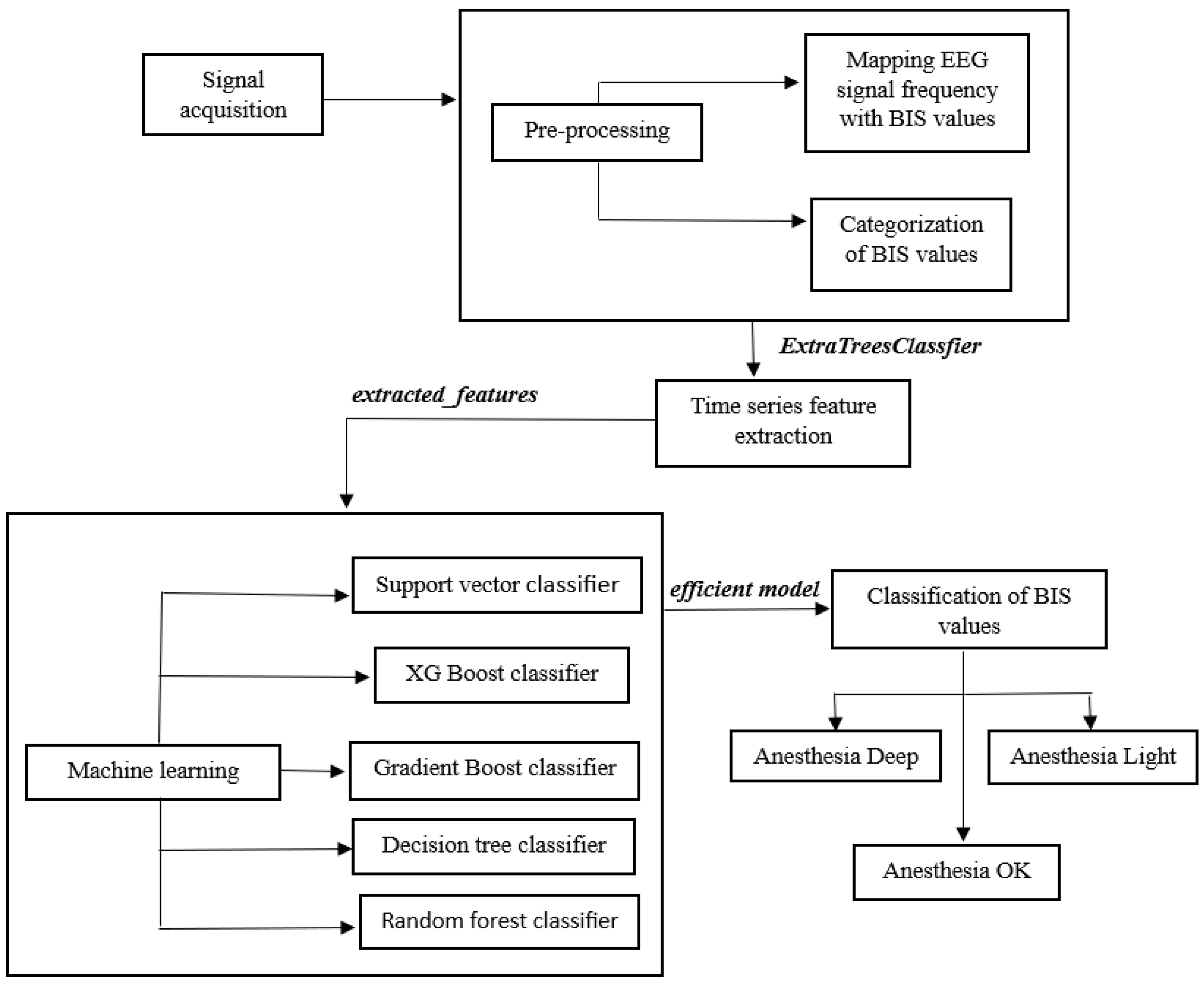
The National Taiwan University Hospital (NTUH) in Taiwan’s Research Ethics Committee gave its approval for this study. Furthermore, patients’ permission was obtained in writing after receiving full disclosure. Data were gathered from 50 patients who underwent various surgeries at NTUH and were in the age group range between 23 and 72. The datasets were processed at 5 s interval period, yielding a little more than 15,000 samples for experimentation. [21,22]. Figure 1 shows the proposed methodology carried out for the study.
The proposed methodology used a time series-based unique approach to classify BIS values using EEG signals, thus monitoring the amount of anesthesia administered to the patient during surgery. This enhanced the safety of the patient by keeping the anesthesia levels in check.
2.1. Data Collection
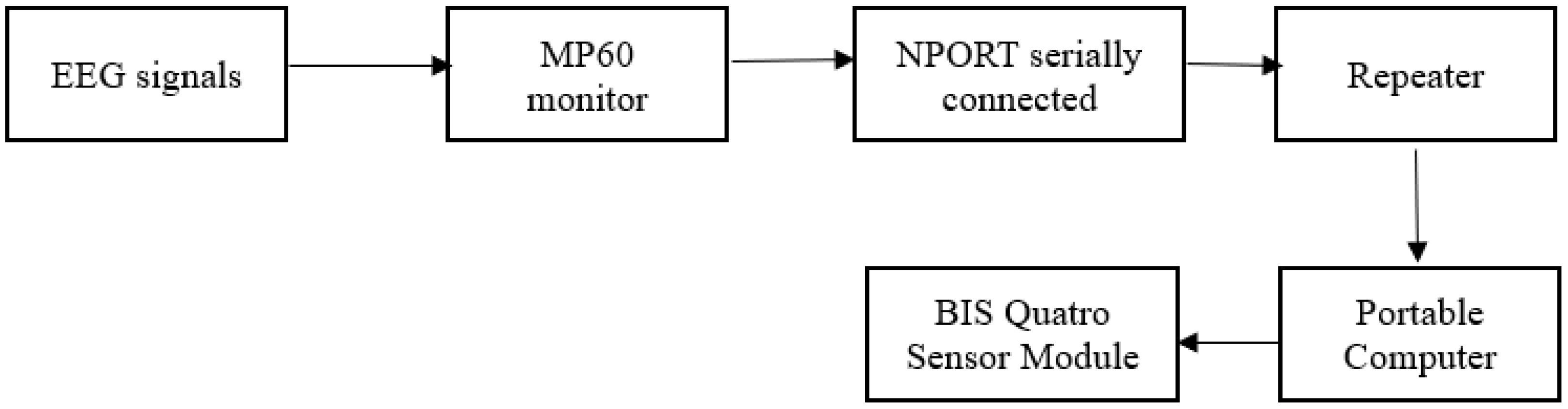
The signals were acquired using a Phillips IntelliVue MP60 physiological monitor, which also had a bi-spectral Index (BIS) quatro sensor, and a portable computer was utilized for logging the data [23]. The MP60 monitor also recorded other vital indications such as heart rate, blood pressure, and SPO2. Additionally, raw PPG, EEG, and ECG signals were also logged. When the patient was undergoing surgery, the BIS monitor provided a numeric variable with a range of 0–100 to determine the anesthetic level, as shown in Figure 2. The EEG signal and the values of BIS were shown on the BIS monitor. Google Colab software was used to analyze the data and build the proposed framework.
Anesthesia Deep, Anesthesia Light, and Anesthesia OK were three categories for the BIS values obtained from the BIS quatro sensor module. The phrase “anesthesia deep” suggested that the patient was too deeply unconscious. Surgery can be performed on the patient if anesthesia is ok. Additionally, anesthetic light suggests that the patient is awake and the surgery cannot continue. The range of BIS values for each category is displayed in Table 1.
During the EEG signal processing, it was found that the data for each DoA level were not uniform, which is why it is frequently claimed that the data sets obtained in the medical field are unbalanced or biased. For purposes of comparison, it is crucial to have datasets of equal sizes for each DoA. Using the same amount of data for each degree of anesthesia is another technique to reduce the data imbalance, which was implemented in this experiment.
2.2. Data Preprocessing
The data need to undergo pre-processing before any feature extraction or machine learning algorithms can be performed. For the signal pre-processing, a 5 s interval was considered because BIS value provided output from the monitor every 5 s. The sampling frequency of the raw EEG signal data was found to be 128 Hz from the MP60 monitor. Thus, we obtained 640 sample points for every 5 s interval corresponding to the BIS value. Therefore, 5 s of 640 points of raw EEG signal sample points were used for further preprocessing. The plot of the raw sampled EEG signal is shown in Figure 3.
Since this was taken up as a time series problem, the sampled signal data were mapped to the corresponding BIS value, according to the categories mentioned in Table 1 (AD, AO, and AL). The mapped data will be used for further pre-processing, i.e., time series feature extraction, which will be discussed in the upcoming sections. Table A1 and Table A2 in the Appendix A shows how the data can be assessed by providing a sample data format after the signal acquisition. Table A1 shows intermittent data for every 5 s and Table A2 shows continuous data set for 128 Hz of EEG signals. A subset of data is shown in the figures. From there, the EEG signals were mapped to the BIS values with respect to the timestamp of signal acquisition before proceeding to time series feature extraction.
2.3. Time Series Feature Extraction
The raw mapped data were not enough to train a prediction model. Therefore, a time series feature extraction procedure was proposed. Time series feature engineering is a labor -intensive procedure because, in order to recognize and extract valuable features from time series, scientists and engineers must take into account the numerous techniques of signal processing and time series analysis.
By combining 63 time series characterization methods, which by default compute a total of 794 time series features, with feature selection based on automatically configured hypothesis tests, the Python package Tsfresh (time series feature extraction on basis of scalable hypothesis tests) streamlined this procedure. Tsfresh closes feedback loops with domain experts and promotes the early development of domain-specific features by detecting statistically important time series characteristics at an early stage of the data science process. These features describe the time series’ fundamental properties, such as the number of peaks, the average or greatest value, or more sophisticated properties such as the time-reversal symmetry statistic. Figure 4 shows the pipeline of the feature extraction process [24].
The time series can be used with the set of features to build statistical or machine learning models that can be used for the problem statement. Time series data frequently include noise, duplication, or unnecessary data. Therefore, the majority of the retrieved features will not be helpful for predicting the anesthetic depth. Tsfresh package has methods to filter and prevent the extraction of pointless features. This filtering process assesses each characteristic’s significance and explanatory power for the specific task at hand. It uses a multiple-test approach and is based on the uses the concept of hypothesis testing. Therefore, the filtering procedure mathematically regulates the proportion of pointless retrieved features. The extract_relevant_feature function was used on the mapped dataset, and by conducting statistical hypothesis tests, a total of 369 time series features were extracted. Some of the features extracted after implementing the above function include: ‘value__number_peaks__n_1’, ‘value__autocorrelation__lag_2’, ‘value__fourier_entropy__bins_100’, ‘value__fft_aggregated__aggtype_”variance”. The list goes up to 369 features, as mentioned before. Furthermore, relevant features are extracted using ExtraTreesClassifier algorithm, which is discussed in the next section.
2.4. Extra-Trees-Classifier for Feature Extraction
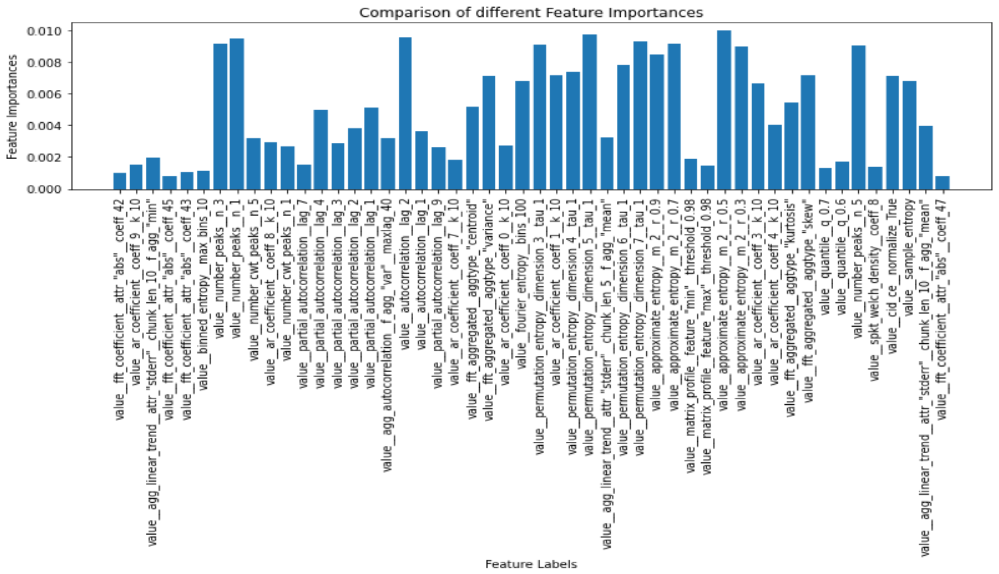
This class implements a meta estimator that employs averaging to increase predictive accuracy and reduce overfitting. The meta estimator fits a number of randomized decision trees (also known as extra-trees) on different sub-samples of the dataset. This technique was further applied to the extracted 369 features to visualize each feature with its importance. The entropy criteria were used in the extratreesclassifier in order to compute the importance, and the normalized feature importance were plotted in the y-axis, while the features were on the x-axis. The term “feature importance” relates to methods for scoring each input feature for a certain model; the scores indicate the “importance” of each feature. A higher score indicates that the particular characteristic will have more of an impact on the model being used to forecast the BIS values and the anesthetic depth.
The number of trees used by the classifier, denoted by estimators, was set as 700, and the entropy criterion was used to extract the importance value of each feature, and since there were two features involved, EEG data and the BIS value, the max_features parameter was set to 2. The feature_importances function was used to compute the importance of each extracted feature. Figure 5 shows a subset of extracted features along with their computed feature importance.
By setting a threshold for the feature importance value, it was possible to vary the number of features that will be selected for the model training and prediction. This was carried out to prevent overfitting of the model. There were 369 features described in the time series package out of which few are extracted using the importance threshold. Value_autocorrelation_lag revealed how the correlation between any two values of the signal changes as their separation changes. Number_peaks feature calculates the number of peaks of at least support n in the time series. Approximate_entropy implements a vectorized approximate entropy algorithm. There are various such features involved in the extraction process which can be referred from [24].
The threshold for the feature importance was set at 0.006 for this experiment, for which 21 of the most important features were extracted and used for training the machine learning models. It is to be noted that this threshold value can be changed, and it was chosen as 0.006 by looking at the extracted feature graph as it was found to be optimal to the layman’s eye. Varying the threshold will increase or decrease the number of features used for the model accordingly.
2.5. Machine Learning to Classify Anesthetic Depth
Following the time series feature extraction process, machine learning algorithms were used to train the model using those features to categorize the anesthetic depth. For every time series that corresponded to a BIS value, a set of features were used as the independent columns, while the BIS value was the dependent column.
2.5.1. Support Vector Classifier
Support vector machine is primarily employed in machine learning classification issues, which is in line with our current problem statement. The SVM algorithm’s objective is to establish the best line or decision boundary that can divide n-dimensional space into the required 3 classes of anesthetic depth (AL, AD and AO), allowing quick classification of fresh data points. A hyperplane is the name given to this optimal decision boundary. SVM selects the extreme vectors and points that aid in the creation of the hyperplane. Radial basis function (RBF) kernel function was used for fitting the model, and the penalty parameter C was given a high value to reduce the risk of misclassification.
2.5.2. XG Boost Classifier
Extreme gradient boosting (XG Boost) is a distributed, scalable gradient-boosted decision tree (GBDT) machine learning framework. It is considered to be one of the top machine learning libraries that are available to solve problems that involve classification and regression. It offers parallel tree boosting; thus, it has the ability to provide efficient solution while classifying the anesthesia level. The hyperparameter tuning was set to solve the multiclass classification problem, in which each observation is given the distinct probability of belonging to each class. The other parameters were assigned to their default values.
2.5.3. Gradient Boost Classifier
Gradient boosting classifiers combines the number of weak learning models to produce a powerful predicting model. Gradient boosting frequently makes use of decision trees. It has the ability to classify complicated datasets, and thus, gradient boosting models are useful to classify anesthetic depth levels, because of the largeness and the complexity of the dataset. With respect to the parameters, 100 boosting stages were performed using friedman_mse criterion, which measures the quality of the split.
2.5.4. Decision Tree Classifier
Decision trees are ideally favored for solving classification problems, which augurs well for this case. It is a tree-structured classifier, where internal nodes stand in for a dataset’s features, branches for the decision-making process, and each leaf node for the classification result of the anesthetic depth levels. The decision node and leaf node are the two nodes of a decision tree. While leaf nodes are the results of decisions and do not have any more branches, decision nodes are used to create decisions based on the features of the dataset in the current problem statement, and have numerous branches, which finally ends in a decision. Gini index criterion is used to perform the classification.
2.5.5. Random Forest Classifier
Random forest is a machine learning algorithm which uses supervised learning. It involves the process of ensemble learning, which is a method of integrating various classifiers to address difficult issues and enhance model performance. Random forest uses multiple decision trees on different subsets of the input dataset and averages the results to increase the dataset’s predictive accuracy. Thus, it is likely that the classification will give a better output than decision tree classifier and is more likely to suit the dataset for classifying anesthesia depth levels. The number of trees in the forest were set to 100, and the Gini index criterion was used to perform the classification. K-fold validation strategy was performed with K = 5 and the repetition of states was set to 3. Cross validation was carried out with accuracy as the performance metric to measure the efficiency.
The described machine learning models were trained over the dataset containing the time series extracted features, and a comparative analysis of all the algorithms were carried out by analyzing their performance metrics.
3. Results
A balanced dataset with respect to the classes was used for training and testing the model. It was split into 80–20 train-test ratio and fed into the machine learning algorithms described in the previous section. The performance metrics such as accuracy, F1 score, precision, and recall were used to evaluate the model. Since the classification was measured in terms of the true positives and true negatives because of the dependent variable being categorical, an ideal method of assessment would be using precision, F1 score and recall. The root mean squared error (RMSE) or mean absolute percentage error (MAPE) would have been a more ideal assessment if the dependent variable was numerical, which was not the case in this problem statement.
where Tp = True positives, Tn = True negatives, Fp = False positives and Fn = False negatives.
Table 2 shows the results of all the algorithms with their performance metrics describing the efficiency of the implemented machine learning models.
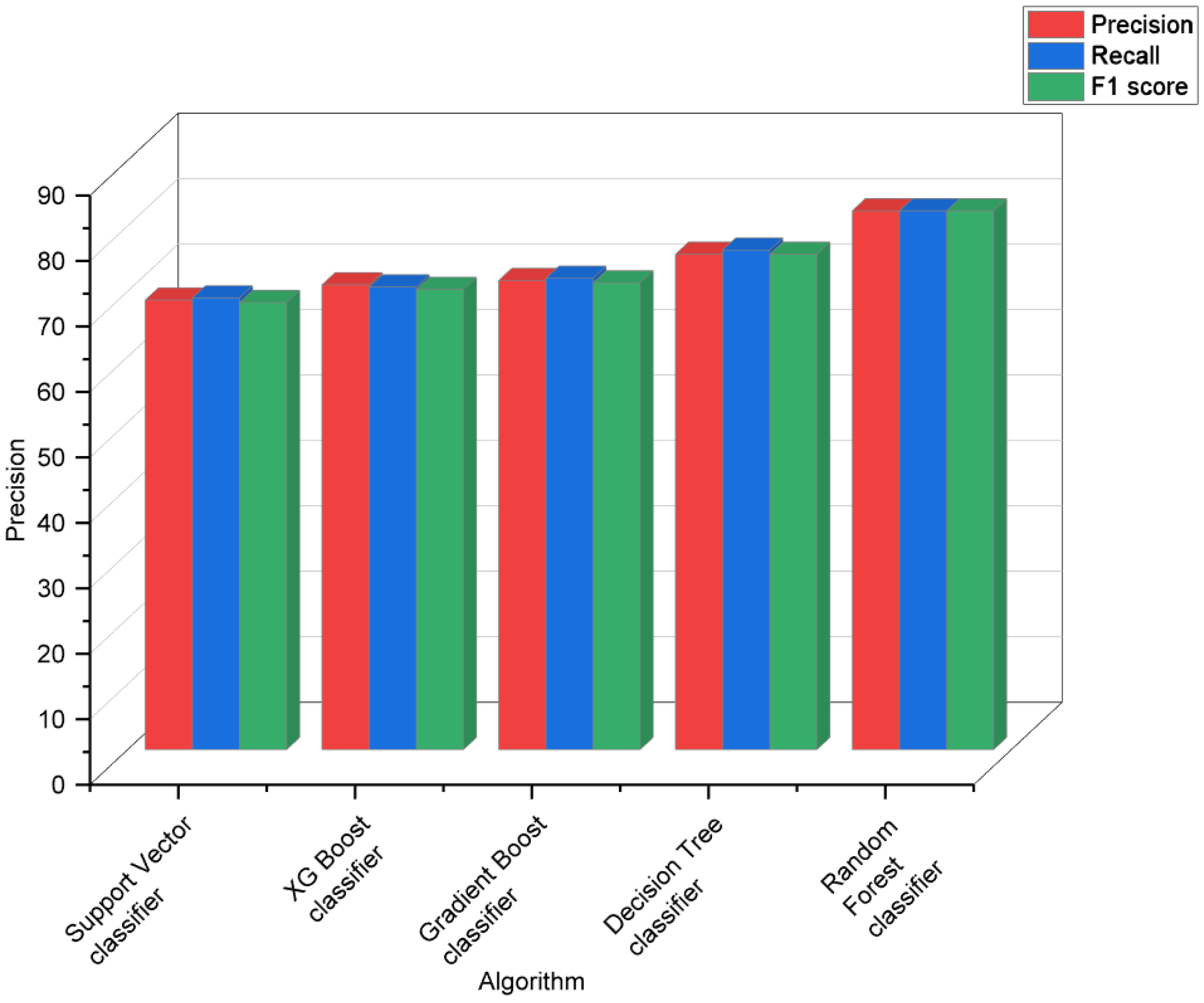
Support vector classifier classified all three classes with an average accuracy of 68.67%, and it equally identified the AD and AL classes. XG Boost classifier classified the AL class the best while having a better recall and F1 score for AD. It gave an average accuracy of 71%. Gradient boost classifier gave an average accuracy of 71.67%, classifying AD and AL the best compared to AO class. Decision tree classifier gave a much better performance by giving an average accuracy of 75.67%, with high precision for the AD class, followed by AL and AO. Random forest classifier gave a high average accuracy of 82.3% and had a high prediction rate for all the three classes.
The results in Table 3 and Figure 6 show a visual representation of the performance metrics obtained for all the algorithms.
The proposed methodology was compared to the various state-of-the-art algorithms with respect to the work carried out by Madanu et al. [21], since the data used in this paper and the referenced work were similar, and thus, it would be more meaningful to compare the results for similar kind of data. The results are described in Table 4 and Figure 7.
4. Discussion
A substantial amount of study was carried out on estimating DoA, and there were some significant advancements in this area. Deep learning models were used to train the dataset by performing different types of pre-processing with the EEG signals. It was noted that many methodical evaluations of DoA were based on traditional processing of the EEG, and a small number of research works demonstrated the visual mapping of the EEG’s properties utilizing the time-frequency domain. This paper proposed a novel approach by using time series feature extraction techniques, and the dataset was trained on various machine learning models to produce good classification results.
It is possible to improve the results by applying deep learning methods such as LSTM after the extraction of time series features. Further pre-processing of the EEG signals may be carried out, such as converting it into the frequency domain, before applying the time series feature extraction technique, which can further enhance the quality of the dataset given for training. Therefore, this paper provided a unique approach in predicting the anesthetic depth, which plays a vital role during a surgical procedure.
Author Contributions
R.V.A. analyzed the data, developed the algorithms and wrote the paper; S.-Z.F., M.F.A. and J.-S.S. evaluated and supervised this study. All authors have read and agreed to the published version of the manuscript.
Funding
This work was financially supported by the Ministry of Science and Technology, Taiwan (grant number: MOST 107-2221-E-155-009-MY2).
Informed Consent Statement
Informed consent was obtained from all participants involved in the study.
Data Availability Statement
Data presented in the paper are available on request from the corresponding author J.-S.S.
Acknowledgments
The authors are grateful to the senior anesthesiologists for their invaluable support in this research, and to all participants who volunteered in the study.
Conflicts of Interest
The authors declare no conflict of interest.
Appendix A

Table A1.
BIS value data format after signal acquisition.
| Timestamp | HR (Beats/Min) | SPO2 (%) | NBP_Dia (mmHg) | NBP_Sys (mmHg) | NBP_Mean (mmHg) | BIS Value |
|---|---|---|---|---|---|---|
| 15–10–2014 12:52:52 | 101 | 100 | 71 | 110 | 81 | 69 |
| 15–10–2014 12:52:57 | 102 | 100 | 71 | 110 | 81 | 65 |
| 15–10–2014 12:53:02 | 100 | 100 | 71 | 110 | 81 | 61 |
| 15–10–2014 12:53:07 | 100 | 100 | 71 | 110 | 81 | 62 |
| 15–10–2014 12:53:12 | 99 | 100 | 71 | 110 | 81 | 63 |
| 15–10–2014 12:53:17 | 99 | 100 | 71 | 110 | 81 | 69 |
| 15–10–2014 12:53:22 | 99 | 100 | 71 | 110 | 81 | 67 |
| 15–10–2014 12:53:27 | 96 | 100 | 71 | 110 | 81 | 63 |
| 15–10–2014 12:53:32 | 97 | 100 | 71 | 110 | 81 | 65 |
| 15–10–2014 12:53:37 | 98 | 100 | 71 | 110 | 81 | 67 |
| 15–10–2014 12:53:42 | 97 | 100 | 71 | 110 | 81 | 63 |
| 15–10–2014 12:53:47 | 95 | 100 | 71 | 110 | 81 | 60 |
| 15–10–2014 12:53:52 | 95 | 100 | 71 | 110 | 81 | 61 |
| 15–10–2014 12:53:57 | 97 | 100 | 71 | 110 | 81 | 61 |
| … | … | … | … | … | … | … |
Table A2.
EEG signal acquisition format.
| Timestamp | EEG (μV) | Timestamp | EEG (μV) | Timestamp | EEG (μV) |
|---|---|---|---|---|---|
| 12:53:02 | 1654 | 12:53:03 | 2146 | 12:53:04 | 2277 |
| 12:53:02 | 1851 | 12:53:03 | 2408 | 12:53:04 | 2637 |
| 12:53:02 | 1687 | 12:53:03 | 1916 | 12:53:04 | 2113 |
| 12:53:02 | 1196 | 12:53:03 | 2277 | 12:53:04 | 1884 |
| 12:53:02 | 1916 | 12:53:03 | 2113 | 12:53:04 | 2441 |
| 12:53:02 | 2146 | 12:53:03 | 1392 | 12:53:04 | 1982 |
| 12:53:02 | 2080 | 12:53:03 | 1818 | 12:53:04 | 2015 |
| 12:53:02 | 2506 | 12:53:03 | 1589 | 12:53:04 | 2506 |
| 12:53:02 | 1949 | 12:53:03 | 1687 | 12:53:04 | 1654 |
| 12:53:02 | 1720 | 12:53:03 | 2310 | 12:53:04 | 2113 |
| 12:53:02 | 2048 | 12:53:03 | 2080 | 12:53:04 | 2310 |
| 12:53:02 | 1359 | 12:53:03 | 2506 | 12:53:04 | 2506 |
| 12:53:02 | 1589 | 12:53:03 | 2572 | 12:53:04 | 3162 |
| 12:53:02 | 1851 | 12:53:03 | 1753 | 12:53:04 | 2867 |
| 12:53:02 | 1785 | 12:53:03 | 1982 | 12:53:04 | 2703 |
| 12:53:02 | 2441 | 12:53:03 | 1556 | 12:53:04 | 2539 |
| 12:53:02 | 2179 | 12:53:03 | 1425 | 12:53:04 | 2113 |
| 12:53:02 | 1949 | 12:53:03 | 1654 | 12:53:04 | 1720 |
| 12:53:02 | 2211 | 12:53:03 | 1851 | 12:53:04 | 1818 |
| 12:53:02 | 1654 | 12:53:03 | 2080 | 12:53:04 | 1196 |
| 12:53:02 | 1949 | 12:53:03 | 2277 | 12:53:04 | 1425 |
| 12:53:02 | 2441 | 12:53:03 | 1654 | 12:53:04 | 2015 |
| 12:53:02 | 2146 | 12:53:03 | 1818 | 12:53:04 | 2015 |
| … | … | … | … | … | … |
References
- Shalbaf, A.; Saffar, M.; Sleigh, J.W.; Shalbaf, R. Monitoring the depth of anesthesia using a new adaptive neurofuzzy system. IEEE J. Biomed. Health Inform. 2017, 22, 671–677. [Google Scholar] [CrossRef] [PubMed]
- Monk, T.G.; Saini, V.; Weldon, B.C.; Sigl, J.C. Anesthetic management and one-year mortality after noncardiac surgery. Anesth. Analg. 2005, 100, 4–10. [Google Scholar] [CrossRef] [PubMed]
- Sebel, P.S.; Bowdle, T.A.; Ghoneim, M.M.; Rampil, I.J.; Padilla, R.E.; Gan, T.J.; Domino, K.B. The incidence of awareness during anesthesia: A multicenter United States study. Anesth. Analg. 2004, 99, 833–839. [Google Scholar] [CrossRef] [PubMed]
- Gugino, L.D.; Chabot, R.J.; Prichep, L.S.; John, E.R.; Formanek, V.; Aglio, L.S. Quantitative EEG changes associated with loss and return of consciousness in healthy adult volunteers anaesthetized with propofol or sevoflurane. Br. J. Anaesth. 2001, 87, 421–428. [Google Scholar] [CrossRef] [PubMed]
- Rampil, I.J. A primer for EEG signal processing in anesthesia. J. Am. Soc. Anesthesiol. 1998, 89, 980–1002. [Google Scholar] [CrossRef]
- Kortelainen, J.; Väyrynen, E.; Seppänen, T. Depth of anesthesia during multidrug infusion: Separating the effects of propofol and remifentanil using the spectral features of EEG. IEEE Trans. Biomed. Eng. 2011, 58, 1216–1223. [Google Scholar] [CrossRef]
- Nguyen-Ky, T.; Wen, P.; Li, Y.; Gray, R. Measuring and reflecting depth of anesthesia using wavelet and power spectral density. IEEE Trans. Inf. Technol. Biomed. 2011, 15, 630–639. [Google Scholar] [CrossRef]
- Lalitha, V.; Eswaran, C. Automated detection of anesthetic depth levels using chaotic features with artificial neural networks. J. Med. Syst. 2007, 31, 445–452. [Google Scholar] [CrossRef]
- Dou, L.; Gao, H.M.; Lu, L.; Chang, W.X. Bispectral index in predicting the prognosis of patients with coma in intensive care unit. World J. Emerg. Med. 2014, 5, 53. [Google Scholar] [CrossRef]
- Aryafar, M.; Bozorgmehr, R.; Alizadeh, R.; Gholami, F. A cross-sectional study on monitoring depth of anesthesia using brain function index among elective laparotomy patients. Int. J. Surg. Open 2020, 27, 98–102. [Google Scholar] [CrossRef]
- Ferenets, R.; Lipping, T.; Anier, A.; Jantti, V.; Melto, S.; Hovilehto, S. Comparison of entropy and complexity measures for the assessment of depth of sedation. IEEE Trans. Biomed. Eng. 2006, 53, 1067–1077. [Google Scholar] [CrossRef]
- Gifani, P.; Rabiee, H.R.; Hashemi, M.H.; Taslimi, P.; Ghanbari, M. Optimal fractal-scaling analysis of human EEG dynamic for depth of anesthesia quantification. J. Frankl. Inst. 2007, 344, 212–229. [Google Scholar] [CrossRef]
- Jospin, M.; Caminal, P.; Jensen, E.W.; Litvan, H.; Vallverdú, M.; Struys, M.M.; Kaplan, D.T. Detrended fluctuation analysis of EEG as a measure of depth of anesthesia. IEEE Trans. Biomed. Eng. 2007, 54, 840–846. [Google Scholar] [CrossRef]
- Shalbaf, R.; Behnam, H.; Sleigh, J.; Voss, L. Measuring the effects of sevoflurane on electroencephalogram using sample entropy. Acta Anaesthesiol. Scand. 2012, 56, 880–889. [Google Scholar] [CrossRef]
- Shalbaf, R.; Behnam, H.; Sleigh, J.W.; Steyn-Ross, A.; Voss, L.J. Monitoring the depth of anesthesia using entropy features and an artificial neural network. J. Neurosci. Methods 2013, 218, 17–24. [Google Scholar] [CrossRef]
- Liang, Z.; Wang, Y.; Sun, X.; Li, D.; Voss, L.J.; Sleigh, J.W.; Li, X. EEG entropy measures in anesthesia. Front. Comput. Neurosci. 2015, 9, 16. [Google Scholar] [CrossRef]
- Mirsadeghi, M.; Behnam, H.; Shalbaf, R.; Jelveh Moghadam, H. Characterizing awake and anesthetized states using a dimensionality reduction method. J. Med. Syst. 2016, 40, 1–8. [Google Scholar] [CrossRef]
- Christ, M.; Kempa-Liehr, A.W.; Feindt, M. Distributed and parallel time series feature extraction for industrial big data applications. arXiv 2017, arXiv:1610.07717. [Google Scholar] [CrossRef]
- Kempa-Liehr, A.W.; Oram, J.; Wong, A.; Finch, M.; Besier, T. Feature engineering workflow for activity recognition from synchro-nized inertial measurement units. In Pattern Recognition, Proceedings of the ACPR 2019, Communications in Computer and Information Science, Auckland, New Zealand, 26 November 2019; Cree, M., Huang, F., Yuan, J., Yan, W.Q., Eds.; Springer: Singapore, 2020; Volume 1180, pp. 223–231. [Google Scholar] [CrossRef]
- Shah, I.; Jan, F.; Ali, S. Functional data approach for short-term electricity demand forecasting. Math. Probl. Eng. 2022, 2022, 6709779. [Google Scholar] [CrossRef]
- Madanu, R.; Rahman, F.; Abbod, M.F.; Fan, S.Z.; Shieh, J.S. Depth of anesthesia prediction via EEG signals using convolutional neural network and ensemble empirical mode decomposition. Math. Biosci. Eng. 2021, 18, 5047–5068. [Google Scholar] [CrossRef]
- Wei, Q.; Li, Y.; Fan, S.; Liu, Q.; Abbod, M.; Lu, C.; Lin, T.-Y.; Jen, K.-K.; Wu, S.-J.; Shieh, J.-S. A critical care monitoring system for depth of anaesthesia analysis based on entropy analysis and physiological information database. Australas. Phys. Eng. Sci. Med. 2014, 37, 591–605. [Google Scholar] [CrossRef] [PubMed]
- Liu, Q.; Ma, L.; Fan, S.; Abbod, M.; Lu, C.; Lin, T.; Jen, K.-K.; Wu, S.-J.; Shieh, J.-S. Design and evaluation of a real time physiological signals acquisition system implemented in multi-operating rooms for anesthesia. J. Med. Syst. 2018, 42, 1–19. [Google Scholar] [CrossRef] [PubMed]
- Christ, M.; Braun, N.; Neuffer, J.; Kempa-Liehr, A.W. Time Series FeatuRe Extraction on basis of Scalable Hypothesis tests (tsfresh—A Python package). Neurocomputing 2018, 307, 72–77. [Google Scholar] [CrossRef]
Figure 1.
Block diagram of the proposed framework.

Figure 2.
Signal acquisition of EEG signals using suitable hardware.

Figure 3.
Raw sampled EEG signal. The x-axis represents the EEG data point count while the y-axis represents the value of the EEG signal at the given data point.
Figure 3.
Raw sampled EEG signal. The x-axis represents the EEG data point count while the y-axis represents the value of the EEG signal at the given data point.

Figure 4.
Features extraction pipeline.

Figure 5.
Extracted features with their importance value.

Figure 6.
Visualizing performance metrics of various algorithms.

Figure 7.
Comparison of various state of the art algorithms.

Table 1.
Anesthesia level classification according to BIS values.
| BIS Range | Anesthesia Level |
|---|---|
| 0–40 | Anesthesia Deep (AD) |
| 40–60 | Anesthesia OK (AO) |
| 60–100 | Anesthesia Light (AL) |
Table 2.
Performance metrics of the implemented machine learning algorithms.
| Support Vector Classifier | |||
| Class | Precision | Recall | F1 score |
| Anesthesia Deep | 73% | 84% | 78% |
| Anesthesia Ok | 60% | 42% | 50% |
| Anesthesia Light | 73% | 81% | 77% |
| XG Boost classifier | |||
| Class | Precision | Recall | F1 score |
| Anesthesia Deep | 75% | 85% | 80% |
| Anesthesia Ok | 62% | 47% | 53% |
| Anesthesia Light | 76% | 80% | 78% |
| Gradient Boost classifier | |||
| Class | Precision | Recall | F1 score |
| Anesthesia Deep | 77% | 86% | 81% |
| Anesthesia OK | 62% | 50% | 55% |
| Anesthesia Light | 76% | 80% | 78% |
| Decision tree classifier | |||
| Class | Precision | Recall | F1 score |
| Anesthesia Deep | 88% | 99% | 93% |
| Anesthesia OK | 65% | 58% | 61% |
| Anesthesia Light | 74% | 72% | 73% |
| Random forest classifier | |||
| Class | Precision | Recall | F1 score |
| Anesthesia Deep | 92% | 99% | 95% |
| Anesthesia OK | 76% | 66% | 71% |
| Anesthesia Light | 79% | 82% | 81% |
Table 3.
Results of all algorithms.
| Algorithm | Precision | Recall | F1 Score |
|---|---|---|---|
| Support Vector classifier | 68.67% | 69.0% | 68.3% |
| XG Boost classifier | 71.0% | 70.67% | 70.3% |
| Gradient Boost classifier | 71.67% | 72.0% | 71.3% |
| Decision Tree classifier | 75.67% | 76.3% | 75.67% |
| Random Forest classifier | 82.3% | 82.3% | 82.3% |
Table 4.
Comparison of algorithms.
| Algorithm | Accuracy (%) |
|---|---|
| 5 Layered Model | 72 |
| 6 Layered Model | 74 |
| 10 Layered Model | 83 |
| AlexNet Model | 74 |
| Pre-Trained VGG16 Model | 80 |
| Pre-trained VGG19 Model | 77 |
| Pre-trained InceptionRESV2 Model | 70 |
| Proposed algorithm (Tsfresh + Machine learning) | 82.3 |
Disclaimer/Publisher’s Note: The statements, opinions and data contained in all publications are solely those of the individual author(s) and contributor(s) and not of MDPI and/or the editor(s). MDPI and/or the editor(s) disclaim responsibility for any injury to people or property resulting from any ideas, methods, instructions or products referred to in the content. |
© 2023 by the authors. Licensee MDPI, Basel, Switzerland. This article is an open access article distributed under the terms and conditions of the Creative Commons Attribution (CC BY) license (https://creativecommons.org/licenses/by/4.0/).
Share and Cite
MDPI and ACS Style
Anand, R.V.; Abbod, M.F.; Fan, S.-Z.; Shieh, J.-S. Depth Analysis of Anesthesia Using EEG Signals via Time Series Feature Extraction and Machine Learning. Sci 2023, 5, 19. https://doi.org/10.3390/sci5020019
AMA Style
Anand RV, Abbod MF, Fan S-Z, Shieh J-S. Depth Analysis of Anesthesia Using EEG Signals via Time Series Feature Extraction and Machine Learning. Sci. 2023; 5(2):19. https://doi.org/10.3390/sci5020019
Chicago/Turabian StyleAnand, Raghav V., Maysam F. Abbod, Shou-Zen Fan, and Jiann-Shing Shieh. 2023. "Depth Analysis of Anesthesia Using EEG Signals via Time Series Feature Extraction and Machine Learning" Sci 5, no. 2: 19. https://doi.org/10.3390/sci5020019