Analysis of Gun Crimes in New York City

Abstract

Violence involving firearms in the USA is a very important problem. As a consequence, a large number of crimes of this type are recorded every year. However, the solutions proposed have not managed to reduce the number of this type of crime. One of the cities with a large number of violent crimes is New York City. The number of crimes is not homogeneous and depends on the district where they occur. This paper proposes to study the information about the crimes in which firearms are involved with the aim of characterizing the factors on which the occurrence of this type of crime depends, such as the levels of poverty and culture. Since the districts are not homogeneous, the information has been analyzed at the district level. For this, data from the open data portal of the city of New York have been used and machine-learning techniques have been used. The results have shown that the variables on which they depend are different in each district.

1. Introduction

Crimes involving shootings are a major problem in the United States. In this sense, it is possible to find data such as the following that show the problem [1]:

• According to a Pew Research Center study, 44% of Americans say they know someone who has been shot, and another 23% say a weapon has been used to threaten or intimidate them or a family member;
• A September 2019 ABC News/Washington Post poll found that six in 10 Americans fear a mass shooting in their community;
• In a March 2018 USA Today/Ipsos poll, 53% of youth aged 13–17 identified gun violence as a “significant concern”, above all other concerns listed in the survey;
• More than 342,439 people were killed by shooting in the United States from 2008 to 2017, which means that one person is killed with a gun in this country every 15 min.

In this article, the situation discussed in the New York City boroughs of Staten Island, Bronx, Brooklyn, Manhattan, and Queens will be studied. The following data allow us to contextualize what the violence involving firearms is like in New York [2]:

• At the end of 2019, a total of 776 shootings were recorded, both mass and non-mass;
• In August 2020, this number had already been exceeded, with a record of 779 shootings in all the districts of the state of New York, with a total of 942 victims, including injuries and deaths;
• According to the statistics, in the last year, shootings have increased by 38% in New York City, and 77% of shooting victims are people of color;
• Currently, shootings in New York City have been on the rise, with firearm attacks having increased since 2020;
• So far this year, the increase in armed violence in New York has reached 32% compared to the previous year, and a total of 51 deaths have been recorded.

In this work, we propose to analyze the characteristics of the incidents that occur in each of the selected districts of New York City to verify if there is a pattern in each district. For this, we have decided to use machine-learning techniques that allow us to obtain predictive models that explain the characteristics of the incidents in the different districts. Therefore, the objective of the study described in this article is to provide and evaluate through prediction models the relationship between the characteristics of shootings in New York City and the district of the city in which each shooting occurs. In particular, we have determined which are the most significant factors when analyzing a shooting, and we have evaluated if there are significant differences between the different districts that determine the behavior of the shooting. The article is structured as follows: Section 2 describes the state of the art. Section 3 describes the data set and its preparation for analysis. Section 4 describes the methods used. Section 5 shows the analyses developed. In Section 6, the results are discussed. Finally, in Section 7, the conclusions and lines of future work are established.

2. State of the Art

There are numerous studies about the shootings that take place in the United States, their cost in lives, and what they imply for the country on a social and psychological level. However, there is a small number of statistical studies on shootings by state and area. Among them, you can find the following studies:

In [3] is described a study carried out in Geek Culture magazine where the database of the Department of Incidents for shootings of the New York Police is used from the year 2006 to 2019, with postal codes based on the longitude and latitude of the events and the population by zip code. As a result, the ZIP codes with the most shootings in the last decade by percentage of population were obtained (in particular, it was found that the top five were made up of Brooklyn neighborhoods and only one from the Bronx, which contradicts the popular belief of the dangerousness of the Bronx versus other neighborhoods). In [4] is described a study carried out by ‘The Trace’ where armed violence in New York is studied using data from the New York Police Department. A map was made of the more than 12,000 shootings recorded by the NYPD between January 2010 and October 2018. As a result, it was found that, the further someone was from a level I or II care facility when they were shot, the more likely they were to die. Given that the most disadvantaged neighborhoods of New York City are the furthest from hospitals with sufficient resources and open 24 h to deal with gunshot wounds, shootings in those neighborhoods are the most likely to end in deaths. In other words, there is a correlation between the New York neighborhood where a shooting takes place and the possibility of surviving it. In [5] is described a study examining the spatial and temporal trends in gun violence in the city of Syracuse with a population of 145,000. Spatiotemporal groups of shots investigated and corroborated by the City of Syracuse Police Department during the years 2009–2015 were obtained. In addition, predictors of areas with increased gun violence were examined using a multi-level zero-inflated Poisson regression using 2010 census data. Two space–time clusters of gun violence were revealed in the city. Higher rates of segregation, poverty, and the summer months were associated with an increased risk of gun violence. Previous shootings in the area were associated with a 26.8% increased risk of gun violence. Gun violence in Syracuse is spatially and temporally stable. This study described in [6] analyzes trends in gun violence in the United States using the frequency as well as spectral density estimation for a non-stationary time series to investigate state-by-state periodicity and periodic behavior changes over time to understand the dynamics of armed violence. Data from the Gun Violence Archive were used. As a result, the periodicity of the incidents, the locations in time where the behavioral changes occur, and the changes in the patterns of armed violence since April 2020 were obtained. In [7] is described a study analyzing the increase in shooting victimization in Philadelphia, New York, and Los Angeles during the 2020–2021 pandemic. It looks at how these crimes were concentrated in gun violence hotspots, and how the increase affected racial and ethnic disparities in gunshot victimization. The study shows that 36% (Philadelphia), 47% (New York), and 55% (Los Angeles) of the observed increase in shootings during the 2020–2021 period occurred in the top decile of census block groups, by aggregate number of shootings, and that the race/ethnicity of the victims in these hotbeds of gun violence were disproportionately Black and Hispanic. In [8] is described a study assessing the trends and risk factors over time for self-reported gun possession among public-school freshmen and sophomores in Chicago, New York City, and Los Angeles. As a result, it is observed that there is a much higher self-reported rate of carrying weapons and a greater burden of exposure to violence in Chicago compared to New York City and Los Angeles. Students’ exposure to violence extended to other stressors such as fighting, perceptions of safety, and other high-risk behaviors. Through the violence index, people at higher risk were classified and the magnitude of their greater probability of carrying a weapon was described. In [9] is described a study analyzing homicides in New York City in the 1990s. Mixed regression models were used, revealing a significant negative effect of the changes in misdemeanor arrests and a significant positive effect of the changes in the prevalence of cocaine on the changes in total homicide rates. Analyses disaggregated by weapon indicate that the effects of misdemeanor arrests and cocaine prevalence arise for weapon-related homicides but not for non-weapon-related homicides. In [10] is described a study where the causes and risk factors are analyzed, to understand armed violence and reduce its incidence in the USA. The Medline and PMC databases and Rayyan statistical software were used, and a variety of common causal and contributing factors were identified, including but not limited to mental illness, suicidal ideation, intimate partner violence, socioeconomic status, distress community, family life, childhood trauma, current or past substance abuse, and access to firearms. In [10] is described a study that analyzes more than 3 million arrests made by the New York City police over 5 years, examining racial disparities and cases in which officers suspected that the person arrested had criminal possession of a weapon. In each case, the probability that the suspect had a weapon was estimated, and it was found that, in more than 40% of cases, the probability of finding a weapon (usually a knife) was less than 1%; it was also found that blacks and Hispanics were disproportionately stopped in these low-hit-rate contexts, a phenomenon that arose due to two factors: (1) lower thresholds for stopping people, regardless of race, in areas of high crime, whose populations are predominantly composed of minorities, particularly public housing; and (2) lower thresholds for detaining minorities relative to whites in similar situations. Finally, it was shown that, with only the 6% of arrests that are statistically most likely to result in the seizure of weapons, one can recover the most weapons and mitigate racial disparities in who is arrested. The work described in [11] is a pilot test of a predictive policing program designed to reduce gun violence conducted in 2013 at the Chicago Police Department. The program included the development of a list of individuals estimated to be at the highest risk of gun violence. The 426 individuals estimated to be at the highest risk of gun violence were analyzed using ARIMA models to estimate the impacts on city-level homicide trends and using propensity score matching to estimate the effects of being on the list on five measures related to gun violence. State and county level predictors of annual rates of gun violence and gun-related casualty rates in the US were spatially analyzed. The models in the study described in [12] hypothesized predictors of gun violence incidence and casualties over four years. Data sources included the Gun Violence Archive (Washington DC, USA) (US gun violence data for 2014–2017), US Census Bureau (socioeconomic, demographic, and geologic characteristics), ICPSR (Ann Arbor, MI, USA) (crime reports), US Geological Survey (elevation data), and US Gun Law and Ownership. Random forest analyses identified additional relevant interaction terms to be included. As a result, we found that urban counties are the strongest predictor of both gun violence incidents and casualty rates. Similarly [13], places characterized by a greater income disparity were also more likely to experience higher rates of gun violence, especially when the high income was combined with high poverty. Likewise, characteristics at the community and state level are strongly associated with armed violence. Gun violence is the highest in counties with an upper median income and higher levels of poverty. However, poverty did not appear to be related to gun violence rates in relatively low-median-income counties.

3. Materials

The data set used describes shooting incidents that occurred in New York City during the year 2020. These data are manually extracted on a quarterly basis and reviewed by the Office of Management Analysis and Planning before being published on the NYC website, NYC Open Data (www.opendata.cityofnewyork.us, accessed on 1 June 2022.), from where they were collected. Each record represents one tripping incident and includes information about the event, including place and time of occurrence. In addition, information is also included related to the demographics of the suspect and the victim.

The set is made up of a total of 664 observations and 19 variables. Of the total variables, 5 are of the interval type, 1 is of the date type, 1 of the hour type, 3 are binary, and 9 are categorical (within which the objective variable is included).

Table 1. Variables of data set.

Variables	Description	Values
Incident_key	Shooting ID Code	Identifier
Borough	District in which the shooting occurred	Staten Island, Queens, Manhattan, Brooklyn, Bronx
Precinct	Police area where the shooting occurred	Identifier
Jurisdiction	Jurisdiction in which the shooting occurred	Identifier
Location Desc	Place/establishment where the shooting took place	Bar/Night Club, Candy Store, Chain Store, Commercial Building, Department Store, Gas Station, Grocery, Hospital, Hotel/Motel, APT Building, PVT House, Restaurant
Statistical murder flag	The shooting has caused deaths	yes, no
Perp age group	Age group of shooter	<18, 18–24, 25–44, 45–64, 65 and more
Perp sex	Sex of the perpetrator of the shooting	male, female
Perp race	Race/Ethnicity of shooter	Asian/Pacific Islander, Black, Black Hispanic, White, White Hispanic
Vic_age_group	Age group of shooting victims	<18, 18–24, 25–44, 45–64, 65 and more
Vic_sex	Victim’s sex	male, female
Vic_race	Race/Ethnicity of the victim	Asian/Pacific Islander, Black, Black Hispanic, White, White Hispanic
Occur_date	Exact date of the shooting	Date
Occur_time	Exact time of the shooting	Time
X_coord_cd	X co-ordinate of the center block for the New York State co-ordinate system	Co-ordinate
Y_coord_cd	Y co-ordinate of the center block for the New York State co-ordinate system	Co-ordinate
Latitude	Latitude co-ordinate for the Global Co-ordinate System	Co-ordinate
Longitude	Longitude co-ordinate for the Global Co-ordinate System	Co-ordinate
New_georeferenced_column	Georeference	Co-ordinate

shows the variables, their description, and their values.

The objective of the work carried out has been to study whether the district where the shooting takes place can define its characteristics, and, for this, the categorical variable ‘Borough’ has been considered as the objective variable.

To analyze the data, it has been necessary to carry out some transformations and operations on them:

(1)

The incident_key variable is an identification code of the incident. It was found to be duplicated in some cases, and duplicate codes were removed. Thus, we went from 664 initial observations to 528 observations.

(2)

The values of the categorical variables have been recoded with numerical values (see

Table A1. Recoding of categorical values.

Set	Category	Values
Borough	Staten Island	1
	Bronx	2
	Brooklyn	3
	Manhattan	4
	Queens	5
Location-desc	Bar/Night Club	1
	Candy Store	2
	Chain Store	3
	Commercial Building	4
	Dept Store	5
	Gas Station	6
	Grocery	7
	Hospital	8
	Hotel/Motel	9
	APT Building	10
	Public Housing	11
	PVT House	12
	Restaurant	13
	Unclassified	99
Statistical_murder_flag	True	1
	False	2
Perp_age_group	<18	1
	18–24	2
	25–44	3
	45–64	4
	65	5
	Unknown	99
Perp_race	Asian/Pacific Islander	1
	Black	2
	Black Hispanic	3
	White	4
	White Hispanic	5
	Unknown	99
Perp_sex	M	1
	F	2
Vic_age_group	<18	1
	18–24	2
	25–44	3
	45–64	4
	65	5
	Unknown	99
Vic_race	Asian/Pacific Islander	1
	Black	2
	Black Hispanic	3
	White	4
	White Hispanic	5
	Unknown	99
Vic_sex	M	1
	F	2

of Appendix A).

(3)

Treatment of missing data:

In interval-type variables (Latitude, Longitude, X_Coord_cd, Y_Coord_cd), there are no missing values. However, in the categorical variables Location_desc (324 observations), Perp_age_group (314 observations), Perp_race (314 observations), and Perp_sex (314 observations), there are missing data. Since these four variables present more than 50% of absent records, a recategorization of them is chosen, since, if they were eliminated, a large amount of information would be lost. Thus, those lines that appear empty are coded as ‘99’. The new variables are: Rep_Location_desc, Rep_Perp_age_group, Rep_Perp_race, and Rep_Perp_sex.

(4)

Treatment of outliers:

In order to study the atypical data, the symmetry of the variables has been analyzed. A variable is symmetric when the symmetry coefficient is between -1 and 1, such that very large values of this coefficient indicate the existence of outliers. In this case, it is observed that the latitude and longitude variables have a symmetry coefficient outside the indicated range of −2.63241 and 2.979341, respectively), which is an indication of atypical data. To treat these cases, the mean absolute deviation (MAD) method has been used since the median of the values is different from 0, and the ‘Absent’ substitution method has also been used so that atypical data are considered missing and thus are able to be treated later. Once applied, the transformed variables are achieved; rep_latitude and rep_longitude present a coefficient between -1 and 1, but missing data appear (54 observations in latitude and 45 in longitude, respectively). To solve this problem, missing data are imputed using a distribution-based method that fills in missing values taking into account the distribution of the variable.

(5)

Selection of variables:

In order to select the variables that have a greater relationship with the objective variable, the R-square selection method has been used, where a random variable is created that determines the minimum level of significance that will be accepted for the variables of the data set (any variable that explains less than the random variable will be eliminated). In this way, the following variables have been rejected: Vic_sex, Statistical_murder_flag, Vic_age_group, Jurisdiction_code, Rep_perp_sex, Occur_date, and New_Georeferenced_Column.

4. Methods

In order to analyze the objective variable, the following set of machine-learning techniques has been selected:

(1)

Logistic regression [14]: This technique makes it possible to study the association between a categorical or binary dependent variable and a set of categorical or continuous explanatory variables. To achieve this, the probability that the independent variable takes one or the other value is modeled based on the possible combinations of values of the independent variables. The result will be a function that allows us to estimate the parameters by maximum likelihood. This method presents the advantage that allows us to quantify the effects of the predictors on the response through the so-called odds ratio that quantify the change in the probability that the estimated variable belongs to one category or another based on the change of category of each variable included in the model.

(2)

Neural networks [15]: This technique makes it possible to obtain underlying relationships in a data set using a model inspired by physical neural networks. The model consists of a set of interrelated nodes of 3 types (input nodes, output nodes, and hidden layers). The input nodes are the independent variables of the model, the output nodes are the dependent variables of the model, and the hidden layers are artificial variables that do not exist in the data. In addition, there is a combination function that allows input nodes to be related to hidden nodes by combining the inputs using weights, and an activation function that defines the output of a node given an input or a set of inputs (for this modifies the result value or imposes a limit that must be exceeded in order to proceed to another neuron).

(3)

Decision tree [16]: It is a prediction model similar to a flowchart, where decisions are made based on the discriminant capacity of a variable. Probabilities are assigned to each event and an outcome is determined for each branch. In this way, it is possible to distribute the observations according to their attributes and thus predict the value of the response variable.

(4)

Random forest [17]: This technique uses a set of individual decision trees, each trained with a random sample drawn from the original training data using bootstrapping. This implies that each tree is trained with slightly different data. In each individual tree, the observations are distributed by bifurcations (nodes) generating the structure of the tree until reaching a terminal node. The prediction of a new observation is obtained by aggregating the predictions of all the individual trees that make up the model.

(5)

Gradient boosting [18]: This technique is based on using a set of individual decision trees, trained sequentially. Each new tree uses information from the previous tree to learn from its mistakes, improving iteration by iteration. To do this, the weights of the observations belonging to the classes of the event of interest are updated through the optimization in the downward direction of a certain loss or error function, managing to give greater relevance in each iteration to the observations misclassified in previous steps. (An attempt is made to minimize the residuals in the decreasing direction by repeating the construction of decision trees, slightly transforming the preliminary predictions.)

Finally, note that cross validation will be used to assess the goodness of fit. To achieve this, the original data are divided into two: one of the parts on which the model will be built and the other on which the results obtained will be validated. This process will be done n times in order to minimize the random factor in the generation of the partitions.

5. Results

5.1. Decision Trees

Several classification trees have been built for each of the data sets:

• Data Set A. Target Variable: Staten Island District

As there is not a large amount of data available, a data partition of 70 training and 30 tests is carried out. The results obtained can be seen in

Table A2. Decision trees—Staten Island District.

Decision Tree	Characteristics	Failure Rate	ROC
Tree 2	Cut point: ProbChisq p-value: 0.25 Max deep: 22 Sheet size: 17 Adjustment p-value: Bonferroni (Before) Deep: Yes	0.019074	0.963
Tree 4	Cut point: Entropy p-value: 0.25 Max deep: 15 Sheet size: 10 Adjustment p-value: Bonferroni (Before) Deep: Yes	0.019074	0.963
Tree 5	Cut point: ProbChisq p-value: 0.25 Max deep: 12 Sheet size: 8 Adjustment p-value: Bonferroni (Before) Deep: Yes	0.010899	0.994
Tree 6	Cut point: Gini p-value: 0.25 Max deep: 8 Sheet size: 6 Adjustment p-value: Bonferroni (Before) Deep: Yes	0.008174	0.989
Tree 12	Cut point: Gini p-value: 0.25 Max deep: 18 Sheet size: 14 Adjustment p-value: Bonferroni(Before) Deep: Yes	0.019074	0.963
Tree 17	Cut point: Entropy p-value: 0.25 Max deep: 8 Sheet size: 6 Adjustment p-value: Bonferroni (Before) Deep: Yes	0	1

of Appendix B. It is used as the selection criteria in order to have a lower failure rate and a higher ROC index. All trees have a high ROC index and a fairly low misclassification rate, although with variations. That is why Tree 17 is chosen as the best model, which presents the following characteristics: entropy cut-off point, maximum depth 8, leaf size 6, and p-value 0.25. To validate the model, different seeds and cross-validation are used, confirming that the best model is Tree 17.

• Data Set B. Target Variable: Borough of the Bronx

The trees created for Data Set B all have a failure rate equal to 0, so the parsimony or simplest tree criterion is used. In this sense, the best decision tree is Tree 20 (the results obtained can be seen in

Table A3. Decision trees—Bronx District.

Decision Tree	Characteristics
Tree 20	Cut point: ProbChisq p-value: 0.20 Max deep: 8 Sheet size: 6 Adjustment p-value: Bonferroni (Before) Deep: Yes

of Appendix B).

• Data Set C. Target Variable: Borough of Brooklyn

The results obtained can be seen in

Table A4. Decision trees—Brooklyn.

Decision Tree	Characteristics	Failure Rate	ROC
Tree 6	Cut point: ProbChisq p-value: 0.25 Max deep: 20 Sheep size: 16 Adjustment p-value: Bonferroni (After) Deep: Yes	0.021739	0.993
Tree 10	Cut point: Entropy p-value: 0.25 Max deep: 16 Sheep size: 10 Adjustment p-value: Bonferroni (Before) Deep: Yes	0.005435	0.997
Tree 5	Cut point: Gini p-value: 0.25 Max deep: 12 Sheep size: 8 Adjustment p-value: Bonferroni;no Deep: Yes	0.013587	0.993
Tree 20	Cut point: ProbChisq p-value: 0.20 Max deep: 8 Sheep size: 6 Adjustment p-value: Bonferroni (Before) Deep: Yes	0.013587	0.993
Tree 16	Cut point: Entropy p-value: 0.25 Max deep: 18 Sheep size: 14 Adjustment p-value: Bonferroni:no Deep: Yes	0.024457	0.998
Tree 8	Cut point: ProbChisq p-value: 0.25 Max deep: 10 Sheep size: 8 Adjustment p-value: Bonferroni (Before) Deep: Yes	0.013587	0.993

of Appendix B. In this case, the erroneous classification rate and the ROC index have been taken as the selection criteria, so that the best model is Tree 10. However, the statistics do not differ much between the models, which is why they are re-evaluated using the parsimony criterion, finding that the model represented by Tree 5 has a depth and a smaller size of leaves than Tree 10 but still presents good values for the previous statistics. Different seeds are tested and the choice made is verified.

• Data Set D. Target Variable: Borough of Manhattan

The results obtained can be seen in

Table A5. Decision trees—Manhattan.

Decision Tree	Characteristics	Failure Rate	ROC
Tree 2	Cut point: ProbChisq p-value: 0.20 Max deep: 22 Sheep size: 17 Adjustment p-value: Bonferroni (Before) Deep: Yes	0.03523	0.99
Tree 4	Cut point: Entropy p-value: 0.25 Max deep: 7 Sheep size: 5 Adjustmen p-value: Bonferroni (Before) Deep: Yes	0.00271	0.999
Tree 12	Cut point: ProbChisq p-value: 0.25 Max deep: 20 Sheep size: 16 Adjustment p-value: Bonferroni (After) Deep: Yes	0.03794	0.981
Tree 6	Cut point: Gini p-value: 0.25 Max deep: 8 Sheep size: 6 Adjustment p-value: Bonferroni: No Deep: Yes	0.00271	0.999
Tree 5	Cut point: Gini p-value: 0.25 Max deep: 12 Sheep size: 8 Adjustment p-value: Bonferroni: No Deep: Yes	0.00271	0.999
Tree 8	Cut point: ProbChisq p-value: 0.25 Max deep: 10 Sheep size: 8 Adjustment p-value: Bonferroni (Before) Deep: Yes	0.01626	0.995

of Appendix B. The best model is Tree 4 since, although other trees such as 6 or 5 present the same values in the erroneous classification rate and the ROC index, following the parsimony criterion, Tree 4 is the simplest and manages to explain the dependent variable in the same way. Different seeds have been applied, and it is verified that it is the best model.

• Data Set E. Target Variable: Borough of Queens

The results obtained can be seen in

Table A6. Decision trees—Queens District.

Decision Tree	Characteristics	Failure Rate	ROC
Tree 5	Cut point: ProbChisq p-value: 0.25 Max deep: 14 Sheet size: 8 Adjustment p-value: Bonferroni (Before) Deep: Yes	0.016304	0.954
Tree 6	Cut point: ProbChisq p-value: 0.25 Max deep: 8 Sheet size: 4 Adjustment p-value: Bonferroni (Before) Deep: Yes	0.002717	0.992
Tree 7	Cut point: Entropy p-value: 0.25 Max deep: 15 Sheet size: 10 Adjustment p-value: Bonferroni (Before) Deep: Yes	0.002717	0.992
Tree 9	Cut point: Gini p-value: 0.15 Max deep: 18 Sheet size: 12 Adjustment p-value: Bonferroni (Before) Deep: Yes	0.013587	0.991
Tree 11	Cut point: Gini p-value: 0.25 Max deep: 23 Sheet size: 15 Adjustment p-value: Bonferroni (Before) Deep: Yes	0.016304	0.991
Tree 19	Cut point: Entropy p-value: 0.25 Max deep: 12 Sheet size: 6 Adjustment p-value: Bonferroni (Before) Deep: Yes	0.002717	0.992

of Appendix B. For this set, the parsimony criterion is used since Tree 6, Tree 7, and Tree 19 have the same misclassification rate and the same ROC index. Therefore, we learn that the best model is Tree 6 with a maximum depth of 8, a leaf size equal to 4, and p-value of 0.25.

5.2. Logistic Regression

Using this technique, the association between the categorical dependent variable and the rest of the variables in the data set is analyzed, as well as the probability that the objective variable takes one value or another depending on the rest of the variables, which allows us to know the characteristics of the shooting incidents by district. Although different variable selection methods could be used (forward, backward, and stepwise) to find out which variables actually contribute to the target variable, however, the number of variables is very small in all data sets, so when selecting variables, the model is oversimplified and information would be lost. That is why logistic regression models have been built without using variable selection methods. Likewise, cross-validation, different data partitions, and seeds have been used.

Table 2. Logistic regression models for New York City boroughs.

Model	Characteristics	Failure Rate	AIC	SBC	ROC	AUC
Set A	Logistic regression Selecting variables: No Data partition: 60, 20, 20 Seed: 12,345	0.257143	630, 2015	1812, 262	1	315
Set B	Logistic regression Selecting variables: No Data partition: 70, 30 Seed: 12,345	0	734, 2343	2167, 502	1	367
Set C	Logistic regression Selecting variables: No Data partition: 70, 30 Seed: 12,349	0	7342, 343	2162, 643	1	366
Set D	Logistic regression Selecting variables: No Data partition: 60, 20, 20 Seed: 12,345	0.15094	632, 169	1818, 984	1	316
Set E	Logistic regression Selecting variables: No Data partition: 70, 30 Seed: 12,345	0	736, 2025	2174, 377	1	368

presents the best logistic regression models for each of the data sets.

5.3. Neural Networks

Several neural networks have been built for each of the data sets except for Set A, whose target variable is the Staten Island District, due to too small a number of observations. In the rest of the cases, neural networks have been built, configuring parameters such as the number of nodes of the hidden layer, the activation function, and the optimization algorithm.

Table 3. Neural networks for the districts of New York.

Set	Seed	Node Size	Activation Function	Optimization Algorithm	Iterations Early Stopping	Error Objective Variable
B	12,345	4	Softmax	QUANEW	10	0.14293
B	43,265	7	Log	LEVMAR	17	0.49966
B	32,567	12	TanH	LEVMAR	40	0.49433
B	12,349	10	Softmax	QUANEW	28	0.13941
C	31,567	8	TanH	LEVMAR	24	0.49999
C	22,367	3	Log	QUANEW	44	0.49138
C	67,453	7	Softmax	QUANEW	12	0.17545
C	11,567	10	Log	LEVMAR	15	0.49998
D	34,512	15	TanH	QUANEW	8	0.49969
D	77,156	5	Softmax	LEVMAR	25	0.00294
D	12,349	9	Log	LEVMAR	40	0.48635
D	45,447	3	TanH	QUANEW	28	0.49965
E	21,219	2	Log	LEVMAR	16	0.49678
E	30,197	8	Softmax	QUANEW	34	0.10472
E	66,897	12	TanH	QUANEW	56	0.09357
E	34,565	4	Log	LEVMAR	22	0.44616

shows the models obtained.

We learn that, for Sets B, C, and D, the best activation function is Softmax and the Quanew algorithm, except for Set D which uses the Levmar algorithm. Other neural networks for the data are defined in the following table,

Table 4. Selection of neural networks for each district.

Set	Model of Red	Node Size	Activation Function	Optimization Algorithm	Failure Rate	Evaluation ROC
B	NET 1	4	Softmax	QUANEW	0.24431	0.83
B	NET 2	7	Log	LEVMAR	0.25757	0.841
B	NET 3	12	TanH	LEVMAR	0.74242	0.711
B	NET 4	4	TanH	Back Prop (mom = 0.01)	0.45833	0.753
B	NET 5	10	Softmax	QUANEW	0.22727	0.842
C	NET 6	8	TanH	LEVMAR	0.49242	0.705
C	NET 7	3	Log	QUANEW	0.39962	0.882
C	NET 8	7	Softmax	QUANEW	0.21780	0.822
C	NET 9	10	Log	LEVMAR	0.20833	0.714
C	NET 10	3	Tahn	TRUST-REGION	0.11363	0.918
D	NET 11	15	TanH	QUANEW	0.85227	0.58
D	NET 12	5	Softmax	LEVMAR		1
D	NET 13	9	Log	LEVMAR	0.14772	0.658
D	NET 14	3	TanH	QUANEW	0.85227	0.407
D	NET 15	3	TanH	Back Prop (mom = 0.01)	0.85227	0.407
E	NET 16	2	Log	LEVMAR	0.16666	0.668
E	NET 17	8	Softmax	QUANEW	0.16666	0.877
E	NET 18	12	TanH	QUANEW	0.09659	0.8
E	NET 19	4	Log	LEVMAR	0.16666	0.767
E	NET 20	12	tanH	TRUST-REGION	0.10416	0.705

.

In this case, the best neural network model is analyzed based on the misclassification rate and the ROC statistic, and the parsimony criterion is used when necessary. In this sense, for Set B, the best model would be Neural Network 5 with 10 nodes. However, if compared with the rest of the neural networks, the values of the statistics do not differ too much from Network 2 and Network 1, so the parsimony criterion is followed and Network 1 with four nodes is chosen as the best model, with the Softmax activation function and the Quanew algorithm. With respect to Set C, the best neural network is Network 10 that uses three nodes, activation function TanH (hyperbolic tangent), and the trust-region algorithm. In Data Set D, Neural Network 12 is the winner with a classification rate equal to 0 and an ROC index equal to 1. Finally, in Set E, Neural Network 18 with 12 nodes is chosen, with a TanH activation function and Quanew algorithm.

5.4. Random Forest

In this technique, models are built with subsamples to obtain the best possible probabilities and ranking. An attempt is made to improve the accuracy of the classification by incorporating randomness in the input variables. Therefore, for each of the values of the objective variable, we will proceed to build various models, configuring the parameters as follows: the number of trees, the number of variables, the size of the nodes, and the number of significance p-values. Likewise, cross-validation has been used with the aim of minimizing randomness in the models.

Table 5. Characteristics of random forest models.

Model	Set	Iterations	Node Size	Number of Variables	Average Failure Rate	Average AUC
Bagging1	A	100	10	13	0.0136	0.99
Bagging2	B	100	12	13	0	1
Bagging3	C	100	15	13	0.0081	0.99
Bagging4	D	100	14	13	0.0380	0.999
Bagging5	E	100	8	13	0.0135	0.999
RandomForest1	A	100	12	8	0.0054	1
RandomForest2	A	100	14	11	0.0054	1
RandomForest3	A	100	16	7	0.0163	1
RandomForest4	B	100	10	6	0	1
RandomForest5	B	100	15	9	0	1
RandomForest6	B	100	8	5	0.0272	1
RandomForest7	C	100	12	11	0	0.99
RandomForest8	C	100	7	12	0	1
RandomForest9	C	100	15	9	0.0217	0.998
RandomForest10	D	100	6	10	0.0163	0.999
RandomForest11	D	100	14	6	0.0217	0.998
RandomForest12	D	100	9	8	0.0217	0.99
RandomForest13	E	100	12	12	0.0054	0.998
RandomForest14	E	100	6	5	0.0326	0.994
RandomForest15	E	100	9	8	0.0108	1

shows the models built.

All the models present similar values regarding the average failure rate and AUC. Taking into account these values as well as the number of nodes and the number of variables, the models shown in

Table 6. Selected random forest models.

Model	Set	Iterations	Node Size	Number of Variables	Average Failure Rate	Average AUC
RandomForest1	A	100	12	8	0.0054	1
RandomForest6	B	100	8	5	0.0272	1
RandomForest8	C	100	7	12	0	1
RandomForest10	D	100	6	10	0.0163	0.999
RandomForest15	E	100	9	8	0.0108	1

have been selected for each data set.

5.5. Gradient Boosting

The number of iterations, the minimum number of observations, and the regularization constant (shrink) are configured in the model. This last parameter normally oscillates between 0.001 and 0.3 (it converges faster the higher its value is, so that if you set it very low, the number of iterations must be increased for it to converge).

Table 7. Gradient boosting models.

Model	Set	Minimum Number of Observations	Iterations	Shrink	Failure Rate	AUC
GradientBoosting1	A	5	200	0.1	0	1
GradientBoosting2	A	10	100	0.03	0.00545	1
GradientBoosting3	A	8	300	0.001	0.25613	0.986
GradientBoosting4	A	4	100	0.3	0	1
GradientBoosting5	B	5	100	0.05	0	1
GradientBoosting6	B	13	500	0.1	0	1
GradientBoosting7	B	5	300	0.01	0.00817	1
GradientBoosting8	B	7	200	0.04	0	1
GradientBoosting9	C	8	300	0.2	0	1
GradientBoosting10	C	5	100	0.06	0.00815	0.999
GradientBoosting11	C	11	400	0.003	0.0625	0.998
GradientBoosting12	C	9	500	0.007	0.00815	0.999
GradientBoosting13	D	13	100	0.1	0	1
GradientBoosting14	D	6	200	0.02	0.00542	1
GradientBoosting15	D	4	400	0.04	0	1
GradientBoosting16	E	8	100	0.3	0	1
GradientBoosting17	E	10	300	0.003	0.02989	0.982
GradientBoosting18	E	4	200	0.07	0	1
GradientBoosting19	E	13	500	0.03	0	1

shows the execution of several configurations in which some parameters are modified. Those models that have a classification error rate equal to 0 and AUC equal to 1 are selected: GradientBoosting4, GradientBoosting5, GradientBoosting9, GradientBoosting15, and GradientBoosting18.

The following

Table 8. Importance of the variables in each district.

Set	Name Variable	Number of Division Rules	Importance
A	Y_Coord_CD	8	1
	Precinct	10	0.9874
	Longitude	11	0.51509
	Latitude	4	0.11659
	Vic_Age_Group	1	0.01146
B	Y_Coord_CD	33	1
	Precinct	63	0.4965
	Longitude	29	0.2609
	Latitude	9	0.0637
	X_Coord_CD	5	0.0214
	Vic_Age_Group	1	0.00727
C	Precinct	30	1
	Y_Coord_CD	48	0.61135
	Longitude	32	0.2736
	X_Coord_CD	6	0.1000
	Incident_key	13	0.06202
	Latitude	8	0.04057
	Location_desc	6	0.03461
	Perp_Age_Group	3	0.02885
	Vic_Age_Group	1	0.02232
	Vic_Race	1	0.00798
D	Longitude	60	1
	Y_Coord_CD	45	0.9158
	Precinct	59	0.90222
	Latitude	17	0.5656
	X_Coord_CD	8	0.4431
	Vic_Race	13	0.1168
	Location_desc	7	0.0788
	Perp_Age_Group	3	0.0709
	Perp_Race	4	0.0636
	Vic_Age_Group	5	0.0473
E	Longitude	72	1
	Precinct	97	0.5829
	Y_Coord_CD	97	0.3996
	Latitude	22	0.1742
	Vic_Race	5	0.0408
	Perp_Race	3	0.0262
	Incident_key	3	0.0249
	X_Coord_CD	1	0.0146
	Perp_Age_Group	3	0.0127
	Vic_Age_Group	2	0.0091

shows the importance of the variables in each district.

5.6. Comparation Models

Next, the best model for each data set is chosen, comparing the winning models for each value of the objective variable:

• Set A. Target Variable: Staten Island District

In this data set, all techniques except neural networks have been used. If the values of the statistics are compared, the best model is gradient boosting with: a minimum number of four observations, 100 iterations, a regularization constant of 0.3, an error rate of 0, and an error rate of 1.

• Set B. Target Variable: District of the Bronx

In this data set, all techniques have been used. If the values of the statistics of the decision tree models are compared, the logistic regression and gradient boosting are identical. However, the gradient boosting model will be chosen (a minimum number of five observations, 100 iterations, and a regularization constant equal to 0.05) because it contains more information.

• Set C. Target Variable: Brooklyn District

In this data set, all techniques have been used. If the values of the statistics are compared, the best model is the random forest with: 100 iterations, seven nodes, 12 variables, a failure rate equal to 0, and an AUC index equal to 1.

• Set D. Target Variable: Manhattan District

In this data set, all techniques have been used. If the values of the statistics are compared, the best model is gradient boosting with: a minimum number of four observations, 400 iterations, a regularization constant of 0.04, an error rate of 0, and an error index equal to 1.40.

• Set E. Target Variable: Queens District

In this data set, all techniques have been used. If the values of the statistics are compared, the best model is gradient boosting with: a minimum number of four observations, 200 iterations, a regularization constant of 0.07, an error rate of 0, and an ROC of 1.

In conclusion, the gradient-boosting technique is winning for all data sets except the set in which the objective variable takes the value Brooklyn, where the best model is the one obtained with the random forest technique.

6. Discussion

The objective set out in the work is to analyze whether the district in which a shooting occurs determines its characteristics. Next, the results obtained in each district will be analyzed.

6.1. Staten Island District

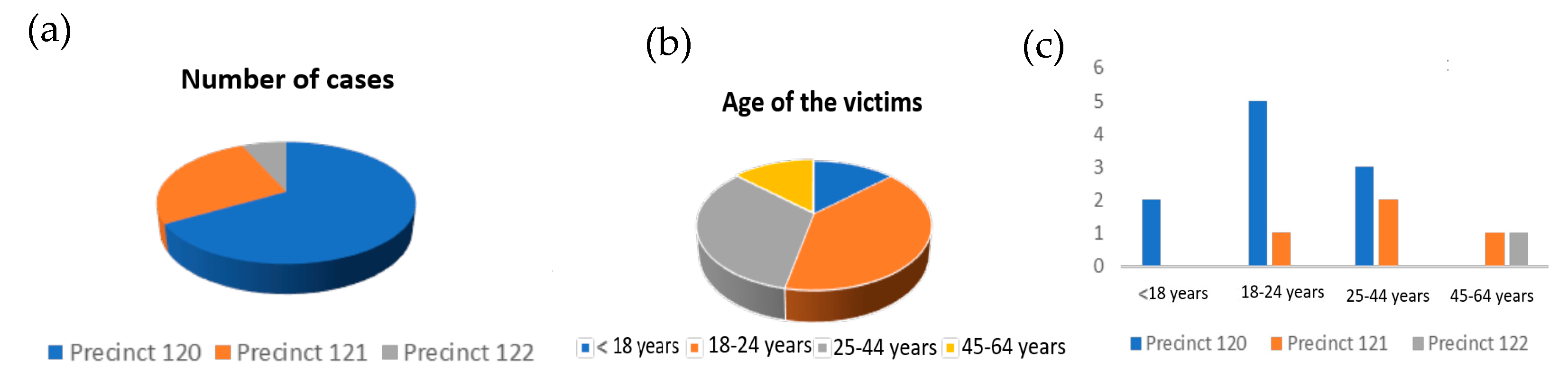
The number of records for this district is minimal and it is observed that the only variable that slightly influences this district is the vic_age_group variable. On the other hand, the precinct variable is of great importance, and allows us to know the areas within the district (Figure 1a) in which the greatest incidents occur. In this sense, it can be seen (Figure 1b) that the most dangerous area within this district is 120, as opposed to Area 122, which would be the safest area. Likewise, it is concluded that most of the victims would be in the range of 18–24 years (Figure 1c). Therefore, given that the average age of the population of the district is 40 years, it can be concluded that the youngest people in this district are the most affected by shootings.

6.2. Bronx District

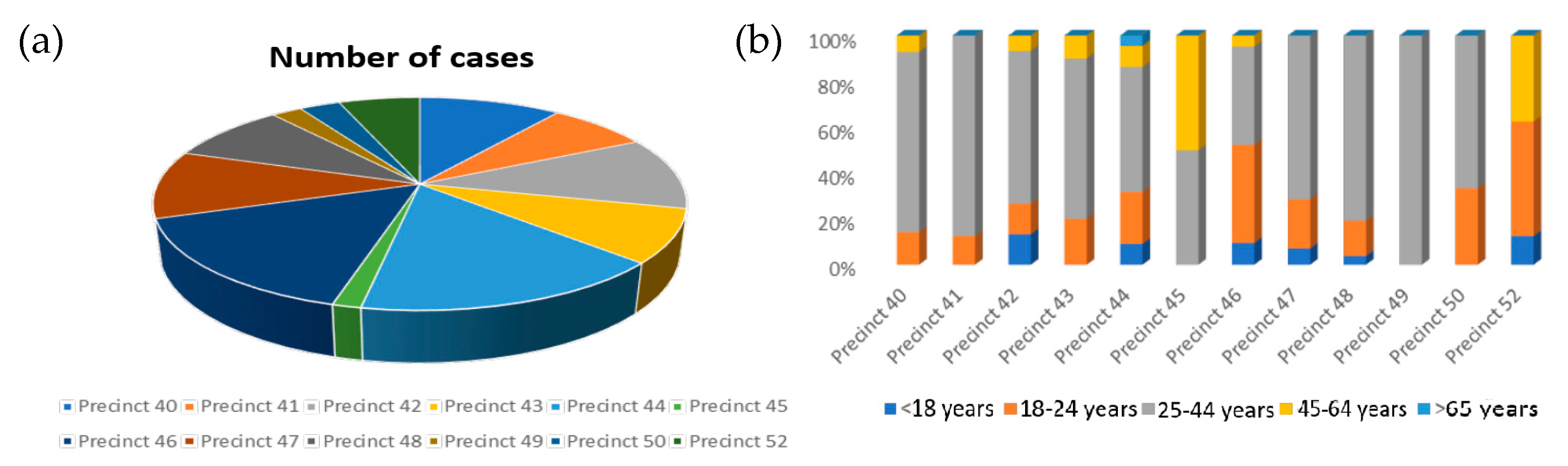
In this district, the influencing variables are precinct and vic_age_group, and it is concluded that the most dangerous areas within the district are Zone 44 and 46, while the safest are Zone 45 and Zone 49 (Figure 2a). Regarding the age of the victims, it is observed that the people most affected in the shootings are those between the ages of 25 and 44 (Figure 2b).

6.3. Brooklyn District

In this district, the only variable that is not important with respect to the study carried out is perp_race. According to Figure 3a, the most dangerous zones are Zones 73 and 75, and the safest zones of the district are 61, 78, and 94. The victims are black people (Figure 3b), and belong to the age range of 25 to 44 years (Figure 3c). Regarding the profile of the attacker, race has no influence but age does. In this sense, the age of the offender (Figure 3d) is in the range of 25 to 44 years without varying in any of the areas of the district. However, in Zones 73 and 75, the age of the offenders is between 18 and 24 years. As for the place where the shootings take place, they usually take place in public or social housing (Figure 3e).

6.4. Manhattan District

In this district, shootings are influenced by the following variables: precinct, vic_race, location_desc, perp_age_group, and perp_race. Figure 4a shows that there are not many differences between the zones within the district, and all maintain a low frequency of shootings except Zone 23, which presents a higher frequency than the rest. Regarding the victims (Figure 4b), it shows that the main victims are black people (in fact, there is a great difference with the rest of the categories). On the other hand, the profile of the attacker (Figure 4c) is a person between 25–44 years of age and black. Another variable that influences this district is the location (Figure 4d), so it can be seen that most of the shootings take place in Zone 23 in public housing.

6.5. Queens District

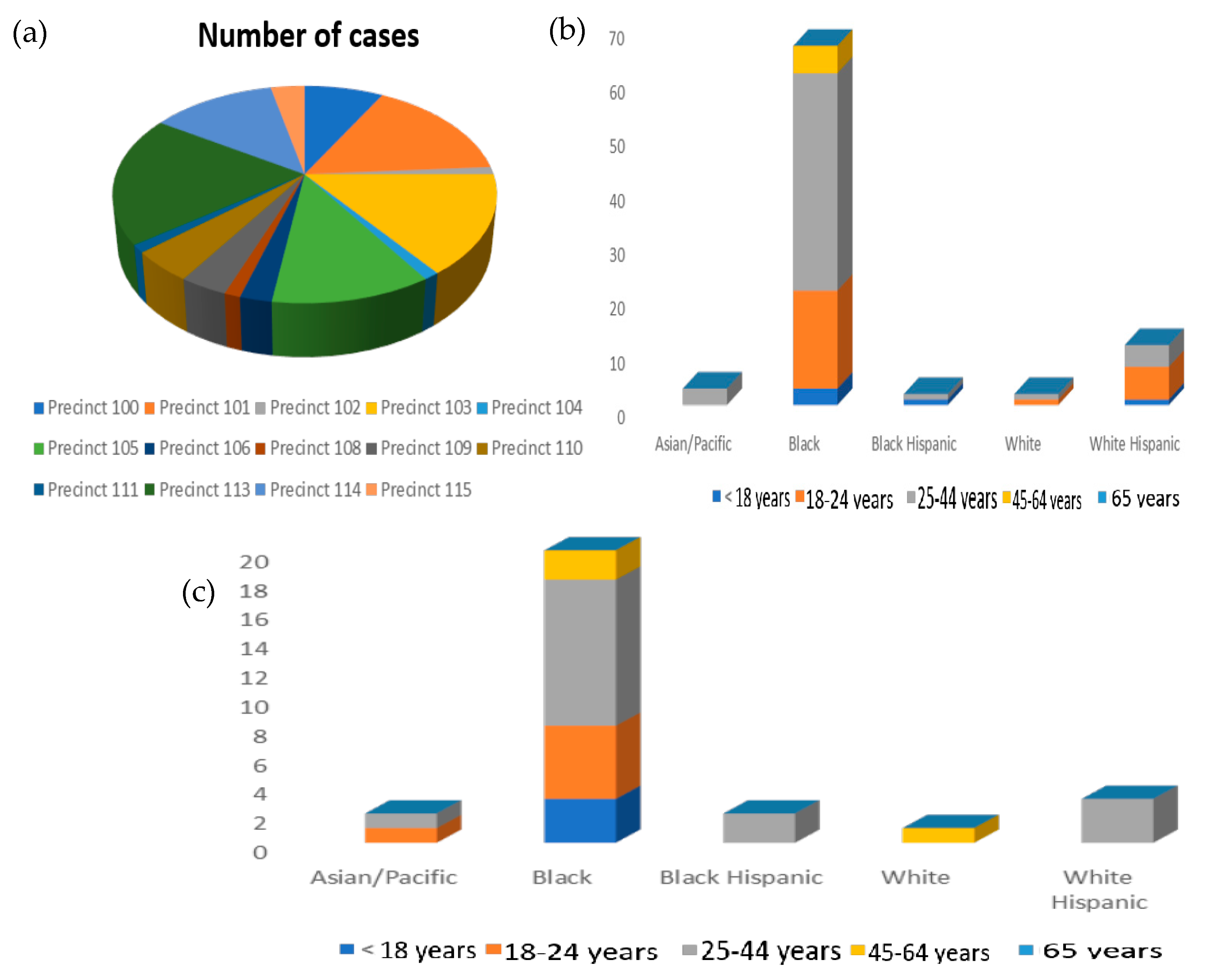
In this district, the location of the shooting does not influence the district, but the following factors do: precinct, vic_race, vic_age_group, perp_age_group, and perp_race. In Figure 5a, it can be seen that the most dangerous areas of the district are Areas 113 and 101, while the safest are Zones 102, 104, 108, and 111. Regarding the characteristics of the victims of the shootings in this district (Figure 5b), it can be deduced that the main victims are black people between 25 and 44 years of age. On the other hand, if the characteristics of the attacker are analyzed (Figure 5c), they have the same characteristics as the victims (people between the ages of 25 and 44, and black).

Finally, note that the main limitations of this work are found in the number of data available and their conditions. In this sense, the work could be improved if a greater number of data were available from various historical series, where more information on the social and economic environment of the people living in each district would be detailed. Likewise, it could be improved if the analysis methods such as the use of convolutional neural networks are expanded.

7. Conclusions and Future Work

In this paper, we have studied the variables that influence crimes involving firearms in New York City with the aim of identifying the areas where most crimes occur, what the victims are like, what the criminals are like, and in what places they occur. An application of this study would allow security, social, and health measures to be taken to reduce the growing number of shootings and thus reduce the number of victims.

The study carried out has shown that there are different behaviors in the districts, and there is no homogeneity that allows us to obtain a single answer. In the Staten Island district, there is a small number of shootings, but they are concentrated in Zone 120. On the other hand, in the Bronx, it has been verified that the most dangerous zones are Zones 44 and 46, and the safest are the 45 and 49. In Brooklyn, the biggest problem is in Zones 73 and 75, and near public housing; moreover, it has been proven that the attackers are usually people whose age is in the range of 25–44 years. This situation is repeated in Manhattan and Queens since they present the same characteristics. In summary, although the district influences the characteristics of the crime, however, a common characteristic is observed with respect to the offenders, who are black people aged between 25 and 44 years.

Note that the factors that define the behavior model in each of the districts are subject to the data analyzed and could change if more data were available to analyze. That is why it cannot be affirmed that, over time, these dependency factors could be different ones.

These results show the need to increase social actions in the most conflictive areas with education and cultural promotion programs such as study aids, increased employability, and social services. According to the results obtained in the work, some security, social, and health measures can be proposed that can reduce the growing number of shootings that have been taking place in New York City since 2019 and that could reduce the number of victims. In the Staten Island district, most of the shootings take place in Area 120, so a plan should be carried out to improve the security of this area by increasing the number of police patrols. On the other hand, in the Bronx, where violence is the order of the day, it has been proven that the dangerous areas are mainly Zones 44 and 46, so work must be done to increase street security in these areas, either by creating more police stations, increasing the patrols to monitor the district, or transferring the existing ones from the safest areas such as 45 and 49. Within Brooklyn, the police presence should be increased in Zones 73 and 75 and near VPO homes, since it is the place where more shootings take place within this district; moreover, it has been proven that the attackers are usually people whose age is in the range of 25–44 years, so focused and attractive social programs should be carried out for people of this age in order to keep them away from violent practices. In addition, these measures could be applied in the same way in Manhattan and Queens since they present the same characteristics regarding the attacker.

In summary, social measures would be necessary to draw attention to young people in this age range (help them to study, increase employability, offer social services, etc.) with the aim of removing them from violent environments. In addition, in those areas where there is a higher rate of shootings, the police presence should be increased, as well as in the buildings where these incidents occur the most (increase in patrols, new police stations, transfers from the safest areas, etc.). Finally, and complementing the increase in police presence, to reduce the number of victims, a health security plan will be carried out, which guarantees that there is a medical center or hospital near the most conflictive areas.

From a political point of view, the results show the need to implement policies to promote culture and social integration in the younger age ranges and among the most depressed and discriminated social classes. These types of policies should be aimed at promoting employment, financial aid for the most vulnerable family groups, study grants, and programs to promote culture, for example, local training programs in new technologies. Likewise, in parallel, the gradual prohibition of firearms or the limitation of access to them should be promoted under very restrictive conditions.

References

- Stansfield, R.; Semenza, D.; Steidley, T. Public guns, private violence: The association of city-level firearm availability and intimate partner homicide in the United States. Prev. Med. 2021, 148, 106599. [Google Scholar] [CrossRef] [PubMed]
- Chalfin, A.; LaForest, M.; Kaplan, J. Can precision policing reduce gun violence? evidence from “gang takedowns” in new york city. J. Policy Anal. Manag. 2021, 40, 1047–1082. [Google Scholar] [CrossRef]
- McArdle, A.; Erzen, T. (Eds.) Zero Tolerance: Quality of Life and the New Police Brutality in New York City; NYU Press: New York, NY, USA, 2001. [Google Scholar]
- Sherman, L.W. Reducing gun violence: What works, what doesn’t, what’s promising. Crim. Justice 2001, 1, 11–25. [Google Scholar] [CrossRef]
- Hosmer, D.W., Jr.; Lemeshow, S.; Sturdivant, R.X. Applied Logistic Regression; John Wiley & Sons: Hoboken, NJ, USA, 2013; Volume 398. [Google Scholar]
- Abiodun, O.I.; Jantan, A.; Omolara, A.E.; Dada, K.V.; Mohamed, N.A.; Arshad, H. State-of-the-art in artificial neural network applications: A survey. Heliyon 2018, 4, e00938. [Google Scholar] [CrossRef] [PubMed]
- Kotsiantis, S.B. Decision trees: A recent overview. Artif. Intell. Rev. 2013, 39, 261–283. [Google Scholar] [CrossRef]
- Shaik, A.B.; Srinivasan, S. A brief survey on random forest ensembles in classification model. In International Conference on Innovative Computing and Communications, Proceedings of ICICC 2018, Manila, Philippines, 5-7 January 2018; Springer: Singapore, 2019; Volume 2, pp. 253–260. [Google Scholar]
- Bentéjac, C.; Csörgő, A.; Martínez-Muñoz, G. A comparative analysis of gradient boosting algorithms. Artif. Intell. Rev. 2020, 54, 1937–1967. [Google Scholar] [CrossRef]
- Larsen, D.A.; Lane, S.; Jennings-Bey, T.; Haygood-El, A.; Brundage, K.; Rubinstein, R.A. Spatio-temporal patterns of gun violence in Syracuse, New York 2009–2015. PLoS ONE 2017, 12, e0173001. [Google Scholar] [CrossRef] [PubMed]
- James, N.; Menzies, M. Dual-domain analysis of gun violence incidents in the United States. Chaos Interdiscip. J. Nonlinear Sci. 2022, 32, 111101. [Google Scholar] [CrossRef] [PubMed]
- MacDonald, J.; Mohler, G.; Brantingham, P.J. Association between race, shooting hot spots, and the surge in gun violence during the COVID-19 pandemic in Philadelphia, New York and Los Angeles. Prev. Med. 2022, 165, 107241. [Google Scholar] [CrossRef] [PubMed]
- Kemal, S.; Sheehan, K.; Feinglass, J. Gun carrying among freshmen and sophomores in Chicago, New York City and Los Angeles public schools: The Youth Risk Behavior Survey, 2007–2013. Inj. Epidemiol. 2018, 5, 12–53. [Google Scholar] [CrossRef] [PubMed]
- Messner, S.F.; Galea, S.; Tardiff, K.J.; Tracy, M.; Bucciarelli, A.; Piper, T.M.; Frye, V.; Vlahov, D. Policing, drugs, and the homicide decline in New York City in the 1990s. Criminology 2007, 45, 385–414. [Google Scholar] [CrossRef]
- Sanchez, C.; Jaguan, D.; Shaikh, S.; McKenney, M.; Elkbuli, A. A systematic review of the causes and prevention strategies in reducing gun violence in the United States. Am. J. Emerg. Med. 2020, 38, 2169–2178. [Google Scholar] [CrossRef] [PubMed]
- Goel, S.; Rao, J.M.; Shroff, R. Precinct or prejudice? Understanding racial disparities in New York City’s stop-and-frisk policy. Ann. Appl. Stat. 2016, 10, 365–394. [Google Scholar] [CrossRef]
- Saunders, J.; Hunt, P.; Hollywood, J.S. Predictions put into practice: A quasi-experimental evaluation of Chicago’s predictive policing pilot. J. Exp. Criminol. 2016, 12, 347–371. [Google Scholar] [CrossRef]
- Johnson, B.T.; Sisti, A.; Bernstein, M.; Chen, K.; Hennessy, E.A.; Acabchuk, R.L.; Matos, M. Community-level factors and incidence of gun violence in the United States, 2014–2017. Soc. Sci. Med. 2021, 280, 113969. [Google Scholar] [CrossRef] [PubMed]
Figure 1.
(a) Number of cases by area—Staten Island District; (b) age of the victims—Staten Island District; and (c) age of victims within Zones 120, 121, and 122.
Figure 2.
(a) Number of cases by area—Bronx district; and (b) median age of the district population.
Figure 3.
(a) Number of cases by area—Brooklyn District; (b) race of the victims by zones—Brooklyn District; (c) age and race of the victims—Brooklyn District; (d) age of the criminal—Brooklyn District; and (e) location where the shooting occurs—Brooklyn District.
Figure 4.
(a) Case numbers—Manhattan District; (b) race of the victims—Manhattan District; (c) age and race of the offender—Manhattan District; and (d) location where the shooting occurred—Manhattan District.
Figure 5.
(a) Number of cases by zone—Queens District; (b) age and race of the victims—Queens District; and (c) age and race of the offender—Queens District.