
Supervised Machine Learning for Refractive Index Structure Parameter Modeling
by
 , , , ,
Antonios Lionis
1,*,
Konstantinos Peppas
1,
Hector E. Nistazakis
2 ,
,
Andreas Tsigopoulos
3,
Keith Cohn
4 and
Kyle R. Drexler
5 1
Information and Telecommunications Department, University of Peloponnese, 22100 Tripoli, Greece
2
Section of Electronic Physics and Systems, Department of Physics, National and Kapodistrian University of Athens, Panepistimiopolis Zografou, 15784 Athens, Greece
3
Division of Combat Systems, Naval Operations, Sea Sciences, Navigation, Electronics & Telecommunications Sector, Hellenic Naval Academy, 18538 Pireas, Greece
4
Physics Department, Naval Postgraduate School, Monterey, CA 93943, USA
5
Atmospheric Propagation, Naval Information Warfare Center Pacific, San Diego, CA 92152, USA
*
Author to whom correspondence should be addressed.
Quantum Beam Sci. 2023, 7(2), 18; https://doi.org/10.3390/qubs7020018
Submission received: 21 April 2023
/
Revised: 24 May 2023
/
Accepted: 25 May 2023
/
Published: 1 June 2023
(This article belongs to the Special Issue Laser-Assisted Facilities)
Abstract
:The Hellenic Naval Academy (HNA) reports the latest results from a medium-range, near-maritime, free-space laser-communications-testing facility, between the lighthouse of Psitalia Island and the academy’s laboratory building. The FSO link is established within the premises of Piraeus port, with a path length of 2958 m and an average altitude of 35 m, mainly above water. Recently, the facility was upgraded through the addition of a BLS450 scintillometer, which is co-located with the MRV TS5000/155 FSO system and a WS-2000 weather station. This paper presents the preliminary optical turbulence measurements, collected from 24 to 31 of May 2022, alongside the macroscopic meteorological parameters. Four machine-learning algorithms (random forest (RF), gradient boosting regressor (GBR), single layer (ANN), and deep neural network (DNN)) were utilized for refractive-index-structural-parameter regression modeling. Additionally, another DNN was used to classify the strength level of the optical turbulence, as either strong or weak. The results showed very good prediction accuracy for all the models. Specifically, the ANN algorithm resulted in an R-squared of 0.896 and a mean square error (MSE) of 0.0834; the RF algorithm also gave a highly acceptable R-squared of 0.865 and a root mean square error (RMSE) of 0.241. The Gradient Boosting Regressor (GBR) resulted in an R-squared of 0.851 and a RMSE of 0.252 and, finally, the DNN algorithm resulted in an R-squared of 0.79 and a RMSE of 0.088. The DNN-turbulence-strength-classification model exhibited a very acceptable classification performance, given the highly variability of our target value (), since we observed a predictive accuracy of 87% with the model.
1. Introduction
The use of LASER communication technology allows the transmission of information within the atmosphere via the propagation of an electromagnetic wave, usually in the near IR band. The proliferation of this technology has been significant in the last decade; it will definitely comprise a key constituent of communications in the future, since the bandwidth requirements will be excessively high to be accommodated by traditional radio-frequency (RF) devices. In contrast with the latter, free-space optical (FSO) communications have (i) smaller size, weight, and power (SWaP) requirements; (ii) high-gain concentrated energy delivered due to the LASER’s narrow beam; and (iii) no licensing limitations, owing to their working wavelength. [1]. However, numerous deleterious factors affect the quality of the transmitted signal of an FSO system, such as the system, geometry, misalignment, and atmospheric losses. A significant phenomenon that causes fading to the optical channel is atmospheric turbulence along the path as a result of inhomogeneities in temperature and pressure due to solar heating and wind [2].
Over the last three years, the Hellenic Naval Academy, in collaboration with the Directed Energy group of the Naval Postgraduate School, has conducted a series of experimental research campaigns focused on the modeling of the performance of a free-space optical link in a maritime environment, as well as modeling the optical turbulence such environments through the refractive-index structural parameter . In [3], a new model was proposed that allows FSO-link-performance estimation over sea and leverages point measurements of environmental parameters. We measured the received-signal-strength indicator (RSSI) of the FSO system and constructed a second-order polynomial using regression modeling to quantify its relation with macroscopic environmental parameters collected by a weather station. In [4], the same experimental setup was utilized to improve the aforementioned model and validate it against real meteorological data. The predicted RSSI values exhibited a reasonably strong correlation with the measurements. Additionally, the Navy Surface Layer Model (NAVSLaM) was used to predict atmospheric turbulence based on the same meteorological data and, thus, it demonstrated a statistical correlation between the refractive-index structural parameter and the RSSI. The NAVSLaM model was developed by the Meteorology department of the NPS and predicts the refractive-index structural parameter based upon mean atmospheric layer properties, with an emphasis on the air–sea temperature difference. In [5], we used an information theoretical method—namely, the so-called Jensen–Shannon divergence, a symmetrization of the Kullback–Leibler divergence—to measure the similarity of RSSI measurements with several probability distributions based on the strength of atmospheric turbulence. Furthermore, the Pearson family of continuous probability distributions was also employed to determine the best fit according to the mean, standard deviation, skewness, and kurtosis of the modeled data. Finally, the Monterey Bay experimental setup of NPS was utilized in [6] to measure the atmospheric turbulence over water and compare the results with the predictions of the NAVSLaM model, as well as to conduct a regression analysis for turbulence predictive modeling based on environmental parameters.
The propagation of LASER beams through the atmosphere suffers from temporal and spatial irradiance fluctuations, known as the phenomenon of scintillation, which can cause severe degradation in laser-link performance. The quantitative method to determine the reliability of such links is through a probability density function (PDF) for these fluctuations, which is related to the turbulence regime (which is either weak or strong). The most common metric of scintillation is the scintillation index (), defined as [7]:
where I the irradiance of the optical wave and is its ergodic value. According to the weak fluctuation theory, the is proportional to the Rytov variance [7],
where the refractive-index structural parameter, a metric for the strength of the turbulence, k = 2π/λ is the optical wavenumber, and L is the path length of the link. A representative model for prediction is the Hufnagel–Valley (HV5/7), where the values of 5 and 7 refer to the atmospheric coherence length (r0) in cm and the isoplanatic angle (θ0) in μrads, respectively, for a wavelength of 0.55 μm,
where A is the level of at the ground level, h the height above sea level and u is the rms value of the wind speed. The shortfall of this model is that it is not considered appropriate for maritime environments [7]. Other models reported in the literature are applicable for turbulence prediction in maritime environments. In this paper, we utilize two such models to estimate the value of in a maritime environment and compare it with the values obtained by using a BLS450 scintillometer.
Although atmospheric turbulence is modeled using micrometeorology, Sadot and Kopeika developed a macrometeorology-based model for turbulence predictions [8]. This model requires standard meteorological measurements obtained from a weather station and was used for experimentally derived ( predictions in previous papers [3,9]. The model accounts for the following: the wind speed (m/s), W; the relative humidity (hPa), RH; the solar flux (Cal/(cm2 × min)), SF; the temperature (Kelvin), T; and the cross-sectional area of the particles (cm2/m3), TCSA. It is given by [3]:
where W(t) is a weight function related to the daytime and promotes higher values around midday and lower values around sunrise and sunset. The weight function is based upon the temporal hour, which relates the times of sunrise and sunset to the actual time [9].
Another model that is applicable to maritime environments and has been extensively validated is the Navy Atmospheric Vertical Surface Layer Model (NAVSLaM), developed by the Meteorology department of the Naval Postgraduate School [10]. The NAVSLaM is based on the Monin–Obukhov similarity (MOS) theory and provides estimations along a vertical profile, from sea level up to 100 m. The MOS theory assumes horizontally homogeneous and stationary conditions, as well as constant turbulent fluxes in momentum and sensible and latent heat with regard to the height [11]. In this model, emphasis is placed on the temperature difference between the air and the sea (ASTD). The required inputs for this model are the wind speed, the air and sea temperature, the humidity, and the pressure. The wavelength range within which the model is valid is 0.3–14 μm. The expression for used by NAVSLaM is given by [12]
where A and B are the partial derivatives of the refractive index with respect to the temperature and specific humidity, respectively, k is the von Kármán constant (≈0.4), Ψ is the integrated form of the respective dimensionless profile function, f(ξ) is an empirically determined dimensionless function, z is the height above the surface, g is the gravitational acceleration, z0T is the height at which the log-z profile T reaches its surface value, rTq is the temperature-specific humidity-correlation coefficient, and ξ a universal parameter given by ([11], Equation (17)):
where θu the virtual potential temperature and z0U the height where the log-z profile of U reaches its surface value. The is estimated by iteratively solving Equations (5) and (6).
For many years, independent studies have been conducted on atmospheric characterization by modeling and forecasting the refractive-index structural parameter inside the surface layer, particularly with regard to its effects on laser-beam propagation in free space. The Naval Research Laboratory (NRL) of the United States has been the leading research organization throughout all these years by executing extensive experimental atmospheric turbulence studies in a laser-communications-testing facility (LCTF) across Chesapeake Bay. Beyond the various demonstrations of laser-communications links at very high data rates, atmospheric characterization has also been investigated [13,14,15]. These studies included both passive (spotlight) and active (laser beam) intensity and angle-of-arrival-based turbulence monitoring. To facilitate their asymmetric studies, the NRL developed a multiple quantum well (MQW) modulating retroreflector, which supports high-rate data transfer with very low power requirements [16]. A second approach is the cat’s eye (CEMRR), which consists of a series of modulators. Both devices are suitable for mobile platforms due to their very small size and weight. A unique analogue FM ship-to-shore optical communications system was utilized in a series of marine-laser-communications trials conducted by the Defense Science and Technology Organization of the Australian DoD to show video and bi-directional voice transmission up to 3 km. During these trials, the previously mentioned MRR devices, loaned by the NRL, were validated [17]. The MIT Lincoln Laboratory deployed an experimental link to assess its performance against various atmospheric conditions. An extensive database of measured refractive-index structural parameter distributions was collected and compared with standard PDFs, such as log-normal and gamma–gamma distributions [18]. In [19], the outcomes of an 11.8-km optical connection were used to study how a laser beam’s strength fluctuated as it traveled through turbulence in the atmosphere. Studies on PDF, fade statistic, and high-frequency spectra were conducted based on the analysis of the measured experimental data. The broadening effect of atmospheric turbulence on a propagating laser beam was studied experimentally in [20]. A laboratory setup with altering parameters, such as temperature, wind speed, and pressure, were used to measure this effect. Finally, a significant number of other research papers present results from experimental turbulence studies on various kinds of terrain, optical path lengths, season of the year, and analysis methods [21,22,23,24].
This paper provides the preliminary results of the HNA’s study for the modeling of the refractive-index structural parameter () over a maritime environment, in collaboration with the NPS and the NIWC Pacific. The initial collected dataset of six macroscopic meteorological parameters and values, acquired during the last week of May 2022, as utilized to model the refractive-index structural parameter by employing regression-machine-learning algorithms. In this way, three types of machine-learning algorithm were employed: a random forest (RF), a gradient boosting regressor (GBR), and two neural networks (a single layer and a deep network). The data were split for training and validation, with 80% of the data used for model training and the remaining 20% for testing the model’s prediction accuracy, using root-mean-squared error (RMSE) and R2 parameters as the performance metrics. The respective percentages of each subset for the single-layer NN were 80%, 10%, and 10%, which correspond to the training, validation, and testing of the model, respectively. The performance results of all algorithms appeared to be very promising (R2 > 0.80). Additionally, a DNN was developed to classify the turbulence strength as either strong or weak.
The remainder of this work is organized as follows. Section 2 provides the background for the statistical learning. Section 3 describes the experimental set-up for the data collection. Section 4 presents the results of the regression analysis and classification using ML algorithms, and Section 5 concludes the paper.
2. Statistical Learning Background
Statistical learning refers to the collection of tools used to understand a certain set of data. Usually, we have some input variables (features, Xi), based upon which we seek to make a prediction or obtain an output (response, Y). Statistical learning assumes that there is some kind of relationship between data that can be modeled [25],
where is an error term that is independent of X and has a mean value of zero. The majority of statistical learning methods are categorized either as parametric, where the form of f is known, or non-parametric, where it is not known. Another important consideration is data overfitting, which can lead to misleading results. Finally, most statistical problems are divided into two types, supervised and unsupervised learning. The former type possesses known response values while training the model, whereas the latter does not. This paper follows a supervised statistical learning method using three non-parametric models, i.e., random forest (RF), a gradient boosting regressor (GBR), and two neural networks (NN), involving a single layer and a deep network.
2.1. Tree-Based Methods
The first two algorithms, namely RF and GBR, are tree-based methods and are suitable both for regression and classification problems. These types of algorithm segment the predictor space of the data into small regions and use the mean or mode value of these regions to make the final prediction of the response value. Since the splitting rules of these regions can be summed up in a tree, these algorithms are known as decision-tree methods [25]. Simple decision-tree methods have proven to be relatively ineffective in terms of accuracy; therefore, more advanced methods exist to deal with more complex data. These include random forests and boosting. The advantages of decision-tree methods include: (1) ease of explanation, (2) better mimicking of the human decision-making process, (3) ease of depiction in graph form, and (4) the ability to handle of qualitative predictors without requiring dummy variables [25].
One method of improvement on simple decision-tree methods is ensemble bagging, in which the training dataset is split into subsets, a decision-tree model is created for each of these subsets, and the overall response is an average of responses from the ensemble of models. An improvement on bagging is random forest, which decorrelates ensembles of trees by making them more independent from each other. Instead of considering the whole set of p predictors for each split criterion, random forest methods select a random subset of m predictors. This random selection is repeated in each split step. Another general approach to improving prediction accuracy is boosting. In contrast with bagging, this approach follows a sequential procedure to train the model by using information from a previously trained tree [25].
2.2. Neural-Network-Based Methods
Neural networks mimic the functionality of the human brain, where human neurons are represented by the nodes and the various connections between them by adjusting weights among the nodes [26]. The node is the fundamental component of a neural network; it receives several xi input signals with a corresponding wi weight and b applied bias, a factor associated with the storage of information. The sum of these signals enters the node, where a certain activation function takes place, and processes the information according to the type of the function. A NN structure is defined in two dimensions, namely the number of layers and the number of nodes in each layer. A NN with only one layer is called a single-perceptron model, whereas a network with multiple layers is called a multiple-layer-perceptron model, or a deep neural network. The best number for each dimension is a matter of research [27].
2.3. ML-Based FSO Predictive Modeling
In order to effectively exploit the capabilities of machine-learning algorithms for scientific applications, it is necessary to possess domain knowledge of the area under research. The optical communications community in general, and the free-space optical communications community in particular, have already utilized ML in a variety of related contexts [28,29,30,31,32,33,34,35]. In collaboration with NPS, the HNA has been extensively engaged in ML-based FSO-performance prediction utilizing the existing experimental setup both locations. In [36], we collected a large data set of local atmospheric parameters and analyzed their effects on the received signal strength of the link by measuring the RSSI parameter. The ML algorithms that we used included a k-nearest-neighbor, a decision tree, a random forest, a gradient boosting regressor, and an artificial neural network. These models were compared using the root-mean-square error (RMSE) and the coefficient of determination (R2) of each model. The analysis revealed an excellent fit for all ML algorithms and indicated that they can significantly improve the prediction of the performance of an FSO compared to traditional regression models. While all five machine-learning techniques had good RSSI prediction accuracy, the ANN approach produced the most accurate model in terms of R2, i.e., 0.94867, while the RF produced the best RMSE values, i.e., 7.37, out of all the techniques. While the three other approaches produced their findings with far less training time, ANN and GBR required a significant amount of computing time. Overall, this work gave a full understanding of the accuracy of RSSI prediction utilizing several machine-learning techniques, which were remarkably accurate in modeling such a connection of intricate systems. In [37], a new approach to the modeling and prediction of the performance of a high-energy laser weapon was proposed, which elaborated on the NPS laser-performance-code scheme. This new approach leveraged artificial neural networks (ANNs) for the prediction of optical turbulence strength. This development made it possible to estimate the performance of HEL weapons in close-to-real time, regardless of location. Finally, in [38], six ML algorithms were compared in terms of prediction. In particular, we used a single neural network, a random forest, a decision tree, a gradient boosting regressor, a k-nearest neighbor, and a deep neural network. This study also investigated the influence of atmospheric turbulence in the availability of a notional FSOC link by calculating the outage probability (Pout) assuming a gamma–gamma (GG)-modeled turbulent channel.
3. Measurement-Systems Overview
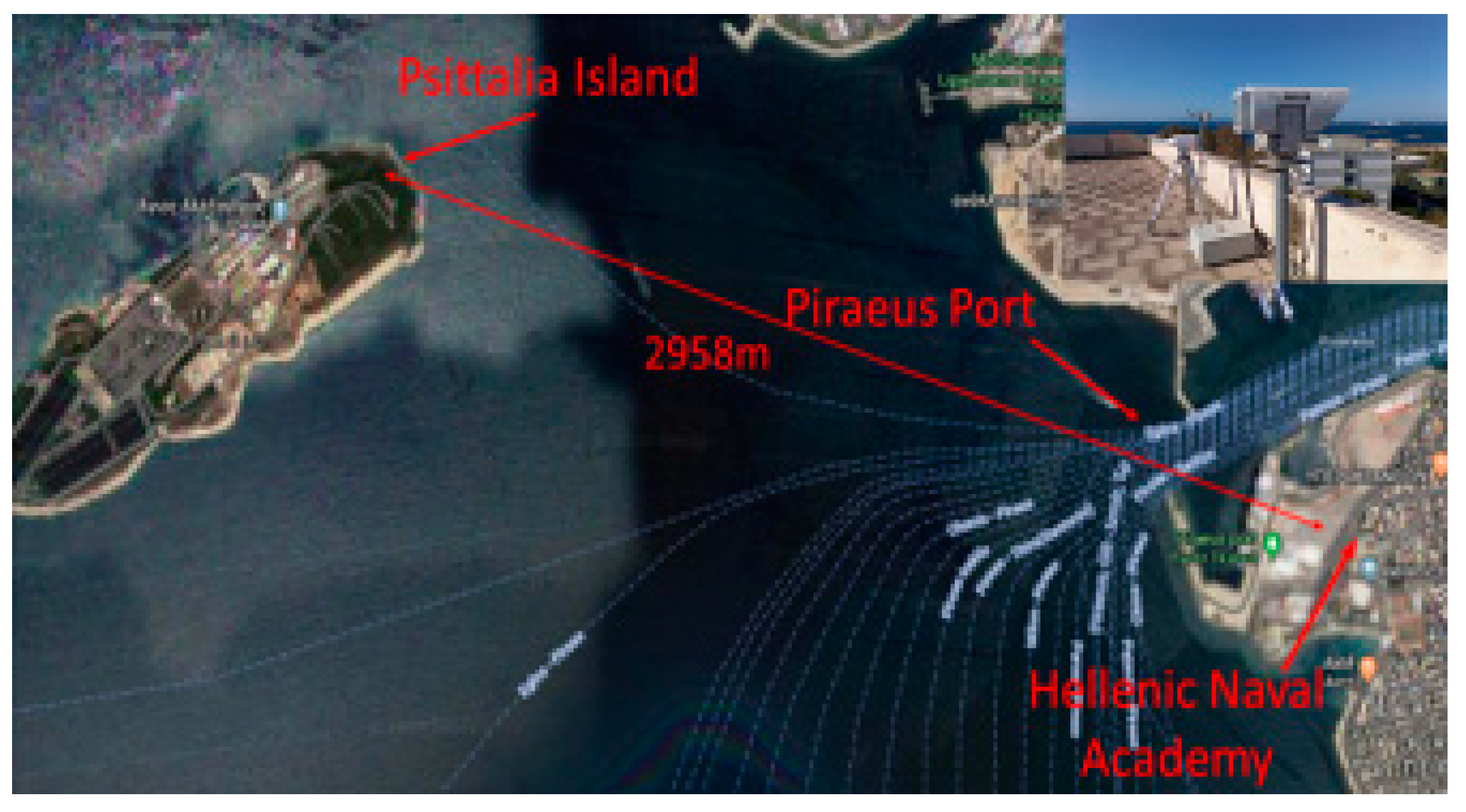
The experimental setup used for this research is located on the HNA premises in Piraeus, Greece. A laser-communications link is established across the entrance of the Piraeus port, between the roof of the laboratory building of the HNA and the lighthouse on Psitalia island, as shown in Figure 1. The total length of the link is 2958 m, most of which is over sea, with a mean value of height above sea level of 35 m.
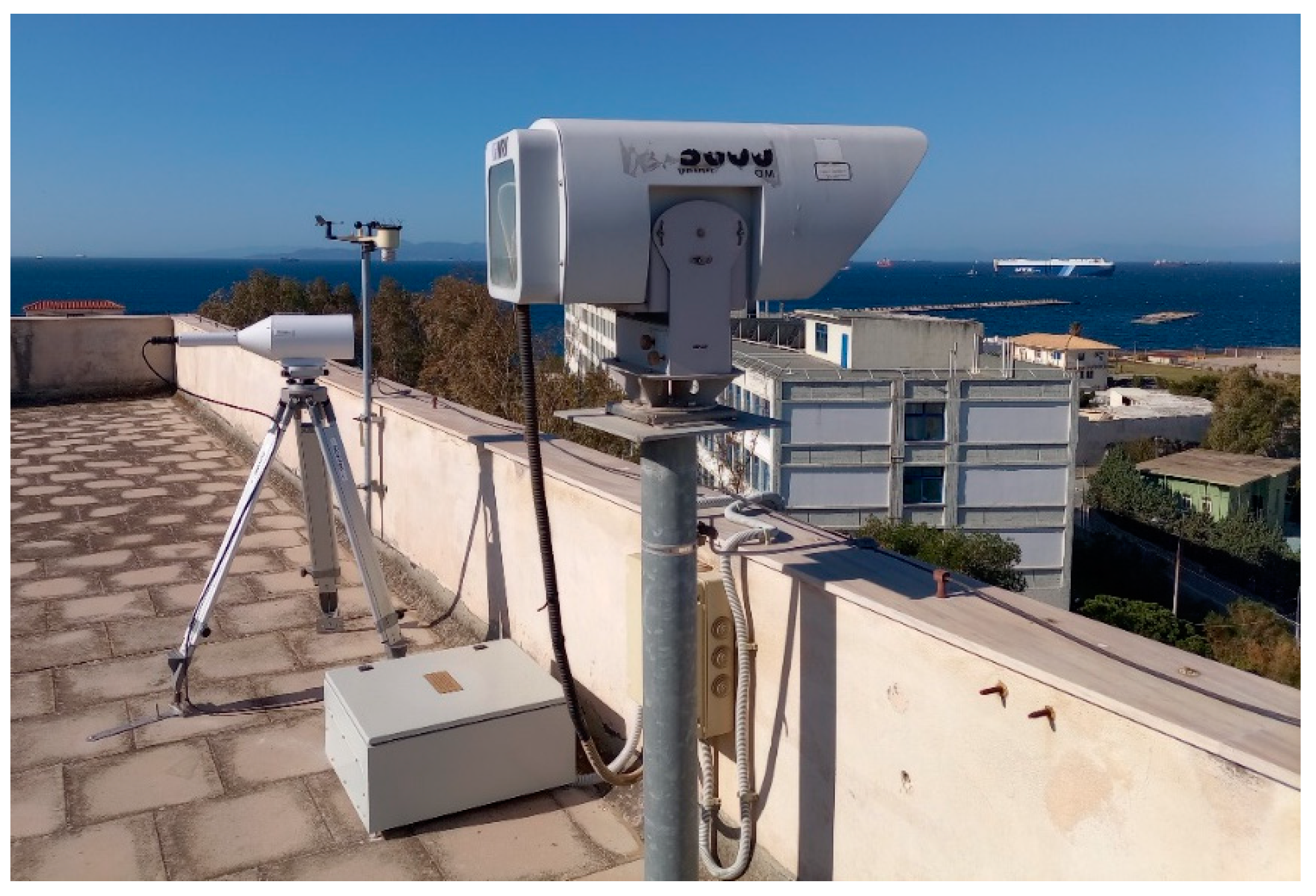
An important pitfall of the setup location is the availability of the link due to the lack of a line of sight whenever a cruise ship is harbored in Piraeus port. The FSO system utilized for the measurements of the received signal was an TS5000/155 model, manufactured by MRV, Israel. The setup consisted of two terminals, one in each location. The operational characteristics of the MRV are available in [3]. Intensity modulation/direct detection (IM/DD) is the system’s scheme, and it operates at a data rate of 155 Mbps. Each FSO terminal measures and indicates the RSSI parameter of the link, which can be stored and exported for further analysis. Beside the MRV system, an Ambient Weather (WS-2000) weather station developed in USA, is located to measure several macroscopic meteorological parameters, including wind speed, wind direction, air temperature, relative humidity, air pressure, dew point, solar radiation, and rainfall rate. Finally, a BLS450 scintillometer, developed by Scintec (Germany), is also located in the vicinity of the MRV and WS-2000 to measure the atmospheric turbulence and heat flux over the path length. A scintillometer measures turbulence along the path between an optical transmitter and a receiver, resulting in a path-integrated Cn2 measurement. Its working theory is based on the scintillation phenomenon, which is the modification of light by changes in atmospheric refractive index. A scintillometer collects spatially representative findings more quickly and with less statistical scatter than traditional turbulence measurements using point sensors. As a double-ended remote-sensing system, the BLS450, also allows access to such terrain (i.e., over water) without the need to install in situ sensors. Figure 2 shows the MRV TS5000/155 FSO system, co-located with the BLS450 scintillometer and the ambient-weather WS-2000, the weather station on the roof of the laboratory building of the Hellenic Naval Academy.
4. Results and Discussion
This paper presents the preliminary results of the experimental measurements that took place during the last week of May 2022 and comprise the first complete dataset from the upgraded instrumentation setup of the HNA experimental site. An initial period of one week (24 to 31 May) was devoted to the data collection and analysis and the ML-based-model construction and validation. Furthermore, the observed meteorological data were used for predictions based on two theoretical models. The main goals of this research analysis were (i) the regression modeling of the refractive-index structural parameter () using ML algorithms and the assessment of their prediction accuracy, and (ii) the application of ML algorithms for the classification modeling of the strength level of the parameter (i.e., low or high).
4.1. Dataset
During the aforementioned period, the observed parameter values from the BLS450 scintillometer were logged once per minute. The same time interval was used for the atmospheric data collection and storage from the WS-2000 weather station in order to accurately match them with the measurements and compile them in an .xlsx file. A few technical issues, such as system resets and line-of-sight link blockages due to maritime traffic, resulted in a few missed measurements. The meteorological conditions during the experiment were quite stable, with air-temperature values ranging from 20 °C to 29 °C, relative humidity within the range of 45–85%, and a very low average wind speed. A key parameter of the meteorological data was the air–sea temperature difference (ASTD). To extract this parameter, we used the online weather statistics database [38]. The entire dataset was screened and redundant recorded data excluded to produce a clean dataset including 8055 rows and eight columns with the meteorological parameters and the respective output value of for the same date/time. As a result, a single approachable file was assembled for additional processing and analysis.
4.2. Regression-Modeling Results
The first part of the analysis was devoted to the modeling of the refractive-index structural parameter by using four machine-learning-based regression algorithms, namely a single-layer neural network, applied in the Neural Fitting application of MATLAB, and a deep neural network, a gradient boosting regressor, and a random forest applied in a Jupyter notebook in the Anaconda environment using the Python language. Two different software-application approaches were followed to compare the prediction accuracy of a built-in model with a user-defined model, which allows much more flexibility.
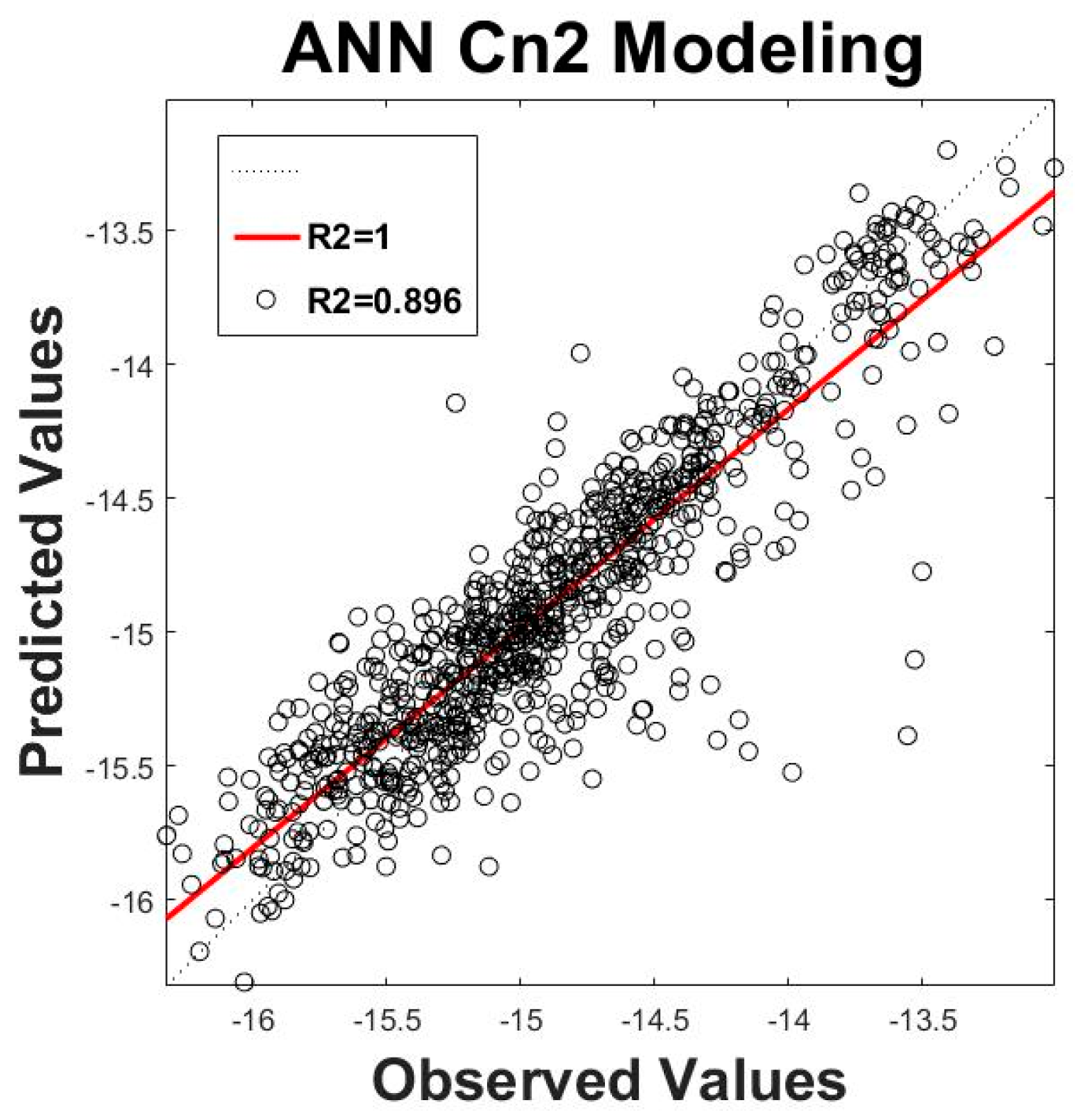
The Neural Fitting application allows data selection and creation, the training of a network, and performance evaluation according to the mean square error and regression analysis. A single hidden-layer feed-forward network with sigmoid hidden neurons and linear output neurons was created in order to fit the seven meteorological parameters (inputs) to the (output). The network was trained either with a Levenberg–Marquardt backpropagation algorithm or with a Bayesian regularization algorithm. The first requires more memory but less time to train the model. As shown by the mean square error of the validation samples, the training automatically ended when the generalization stopped improving. The second technique takes longer, but it can produce strong generalization for challenging, constrained, or noisy datasets. Training stops according to adaptive weight minimization. The network was trained several times using different training algorithms (Levenberg–Marquardt and Bayesian regularization) and numbers of nodes. The best outcome came from a network with 70 nodes, trained with a Levenberg–Marquardt algorithm, which resulted in an R-squared of 0.896 and a mean square error (MSE) of 0.0834. The R-squared measures the correlation between outputs and target values. The closer its value to 1, the closer their relationship. The MSE is the average of the summation of the squared difference between the actual output value and the predicted output value. The goal is to minimize the MSE as much as possible. The data followed an 80/10/10 split for the training, validation, and testing. The results of the network fitting are shown in Figure 3.
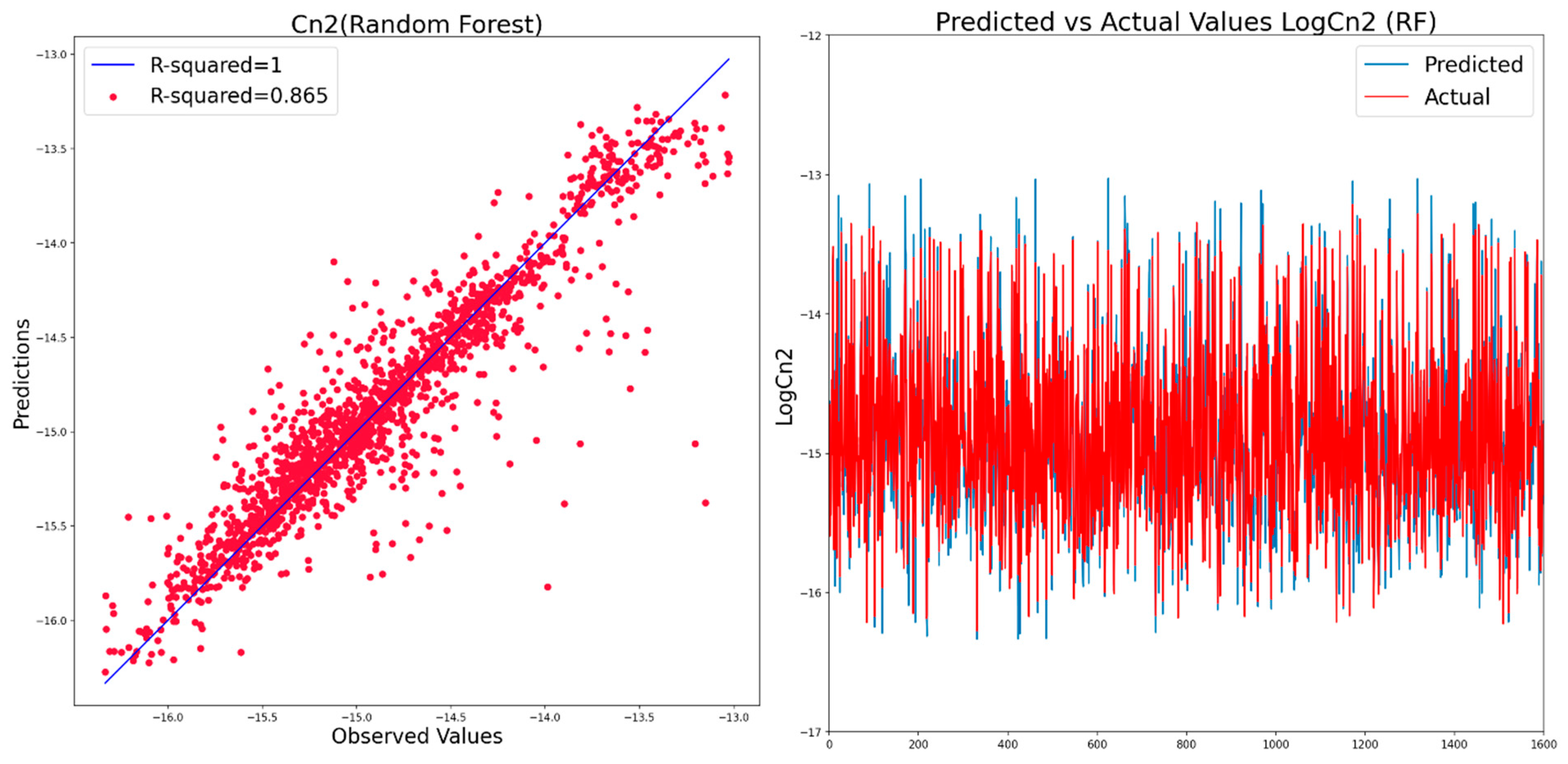
To develop the random forest model, we used the sklearn module and, specifically, the RandomForestRegressor function. Several different parameters can be selected for a RF model. In our case, after executing a grid search and cross-validation, we found the optimal set of the following parameters, the number of decision trees that run in the model (n_estimators = 80), the criterion (loss function) used to determine the model outcome (criterion = MSE), the maximum possible depth of each tree (default value allows leaves’ expansion until they are all pure) and the maximum number of features under consideration in each split (equal to the number of estimators). The results showed a very good agreement between model predictions and observed values, i.e., an R-squared of 0.865 and a root mean square error (RMSE) of 0.241, which are plotted in Figure 4.
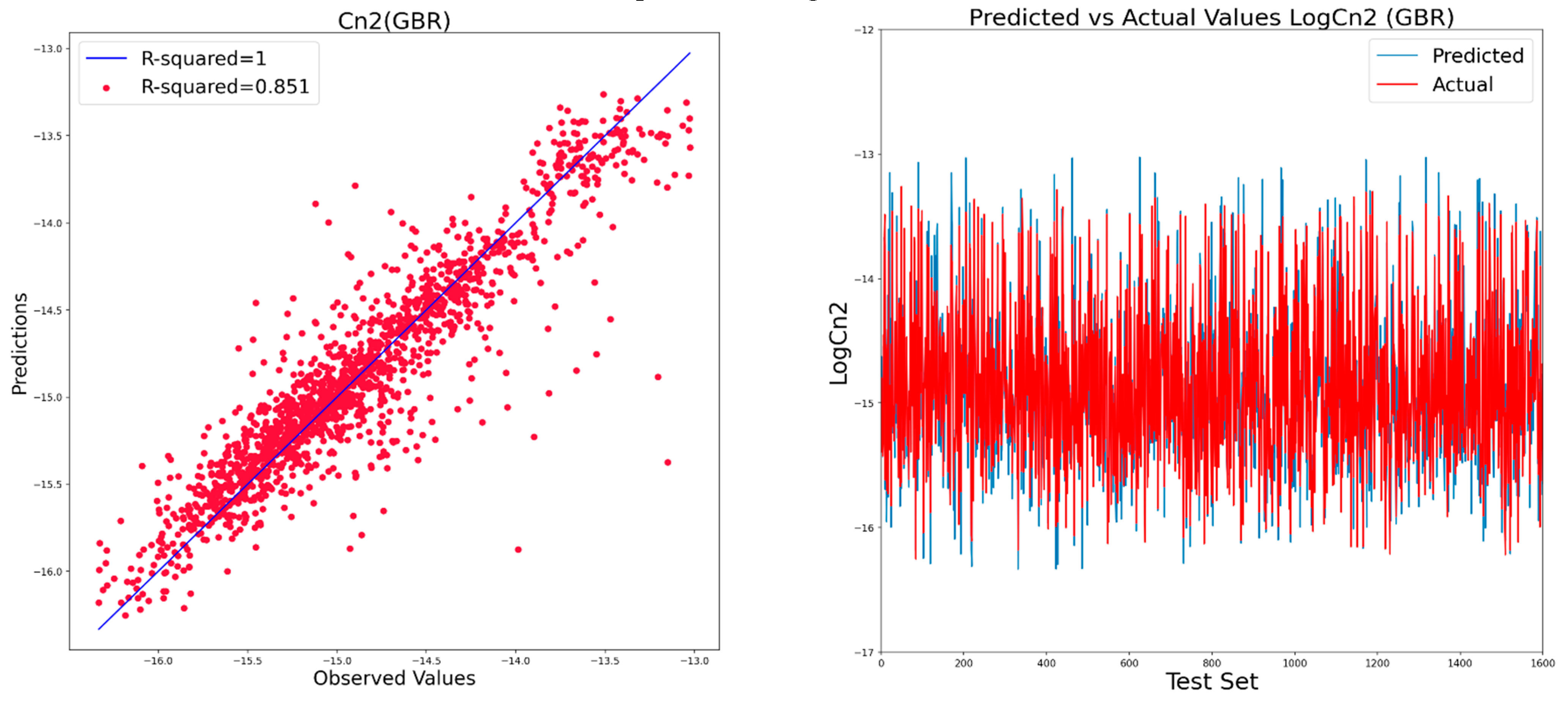
Gradient boosting (GB) is one of the variants of ensemble methods in which weak learners are created in series in order to produce a string ensemble model. It makes use of the residual error for learning. The main training steps for a GB model are as follows: (i) an initial tree estimates the label value; (ii) subsequently, the residual error is calculated; (iii) next, another model is created to predict the error based on the previous model, not the label; and (iv) the label prediction is updated based on the error prediction. Again, the GB model includes several hyperparameters that can be initially selected and tuned adequately. The hyperparameters selected for this model were (i) the number of boosting stages to perform (n_estimators = 1000), (ii) the learning rate of the model (learning_rate = 0.05), (iii) the maximum depth of the individual regression estimators (max_depth = 6), and (iv) the minimum number of samples required to split an internal node (min_samples_split = 12). The results again showed good agreement between the model predictions and the observed values, i.e., an R-squared of 0.851 and a root mean square error (RMSE) of 0.252. These are plotted in Figure 5.
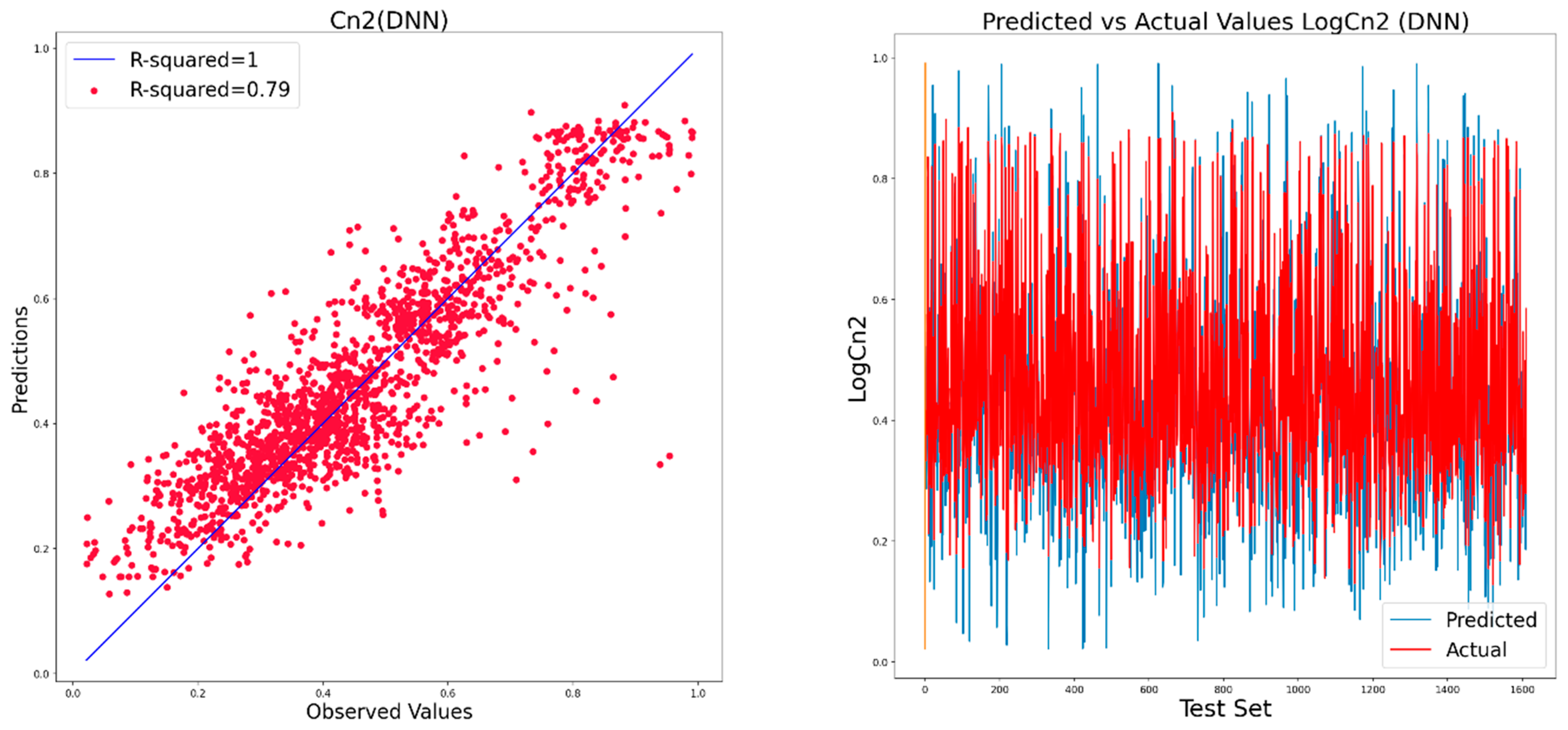
The last algorithm explored was a deep neural network, the evolution of a single-layer network in order to overcome inherent limitations. Practically, a deep neural network is a single neural network with added hidden layers. The number of hidden layers and the number of nodes in each layer control the neural network model’s capacity and depend on the specific problem to be solved. As the dataset was not excessively large, we limited the number of layers in the deep-learning model in order to save time and avoid overfitting. For this model, a three-hidden-layer architecture with a sequentially decreasing number of nodes in each layer (30/20/10) was selected and run over batches of 16 for a total number of 350 epochs. A ReLU activation function was used to connect the hidden-layer nodes and a linear function was used for the output node, because this was a regression model. The ReLU activation outputs the input directly if it is greater than 0; otherwise it returns zero. The loss function (Figure 6) was based on the mean squared error with an Adam optimizer. The line plot shows the expected behavior. The model rapidly learned the problem, decreasing the loss function down to about 0.01 in about 75 epochs, and remained quite stable thereafter. The line plot also shows that the training and testing performances remained comparable during the training, whereas the training line was slightly bumpy. Figure 7 presents the scattering and line plots for the DNN algorithm. The results obtained with this model were R2 = 0.79 and RMSE = 0.088.
4.3. Turbulence-Classification Modeling
To develop a mathematical model for the probability density function (pdf) of the received irradiance, several investigations were carried out. The result of these studies was the development of various statistical models for the scintillation induced by the atmospheric turbulence for a range of atmospheric conditions. The turbulence strength was divided into two levels, weak and strong, defined by the value of the Rytov variance, For values less than unity, the statistics of irradiance can be adequately described by the log-normal model [39]. In cases of higher turbulence strength, the log-normal pdf is not as accurate; therefore, it is not appropriate for strong-turbulence-level irradiance modeling. For higher than unity, the statistics for the received irradiance can be effectively described by the negative exponential or the gamma–gamma pdf. In addition to these two models, numerous others exist can sufficiently describe all the irradiance statistics in either turbulence level or some in both [39].
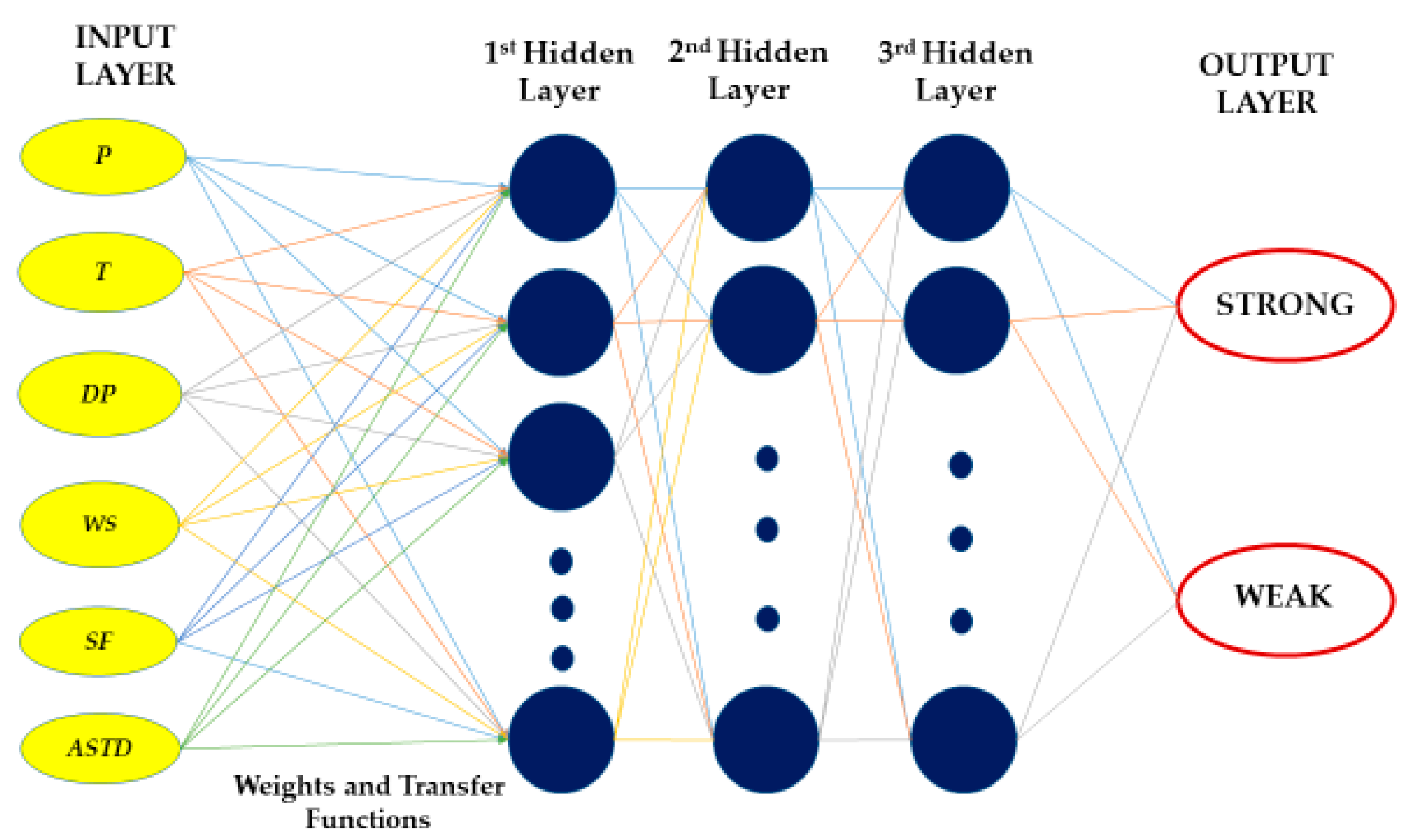
This section aims to describe the use of a DNN approach to model the turbulence-strength level, which is either strong or weak. In this way, we can use the applicable statistical model to describe the channel based on its current status. In order to achieve this, we used the environmental dataset mentioned in Section 4.1 and created the deep neural network shown in Figure 8 to categorize the strength of the turbulence as strong or weak.
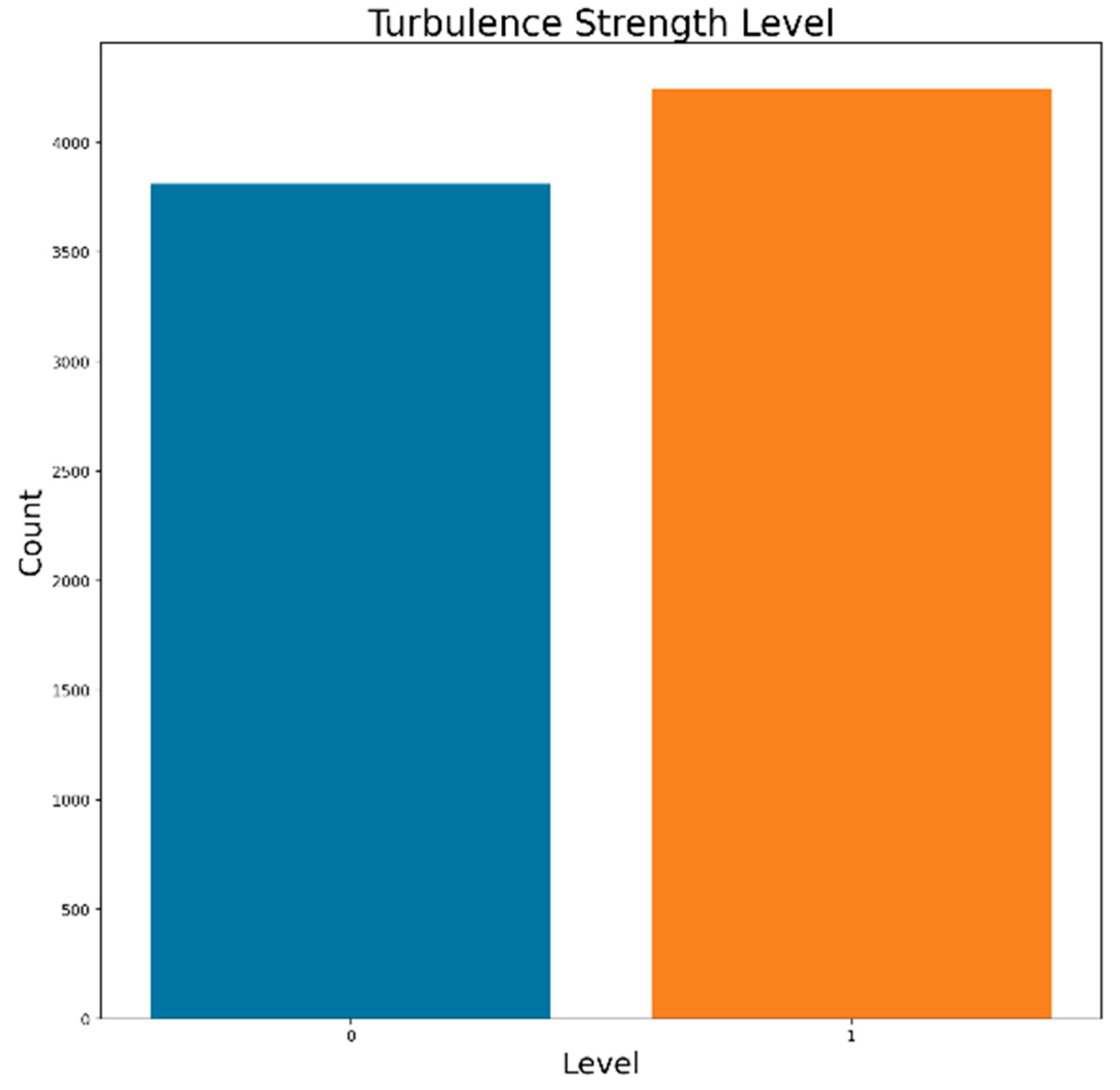
In the raw dataset described in Section 4.1, we assumed a notional value of refractive-index structural parameter, , to characterize it as strong and for weak. Given Equation (2), for , λ = 850 nm, and L = 3000 m, . Therefore, a “0” was attached to every row in our dataset, with and a “1” for . The resulting split in our experimental data was quite balanced and showed that the strong values slightly outnumbered the weak values, as shown in Figure 9.
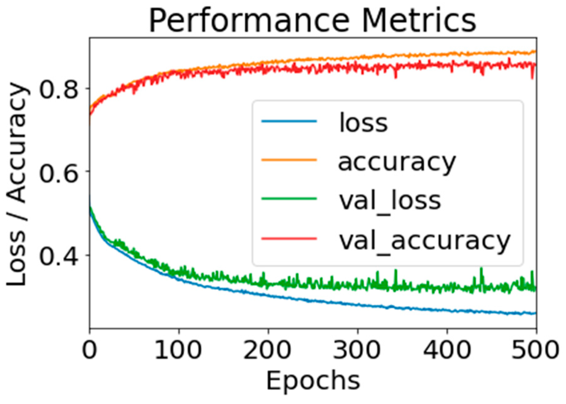
There were three hidden layers in the network, each containing 30 neurons, 20 neurons, and 10 neurons. A dropout rate of 0.5 per layer was utilized using a feed-forward back-propagation technique. For the three hidden layers, the activation function was a rectifier (ReLU), but for the output layer, it was a sigmoid function. In order for the algorithm to monitor the progress of the algorithm fitting, a binary cross-entropy loss function was used and the Adam optimizer was applied to adapt the gradient descent of the loss function. The algorithm was trained against 80% of the dataset and tested over the remaining 20%. We used a total number of 500 training epochs for a batch size of 8. Figure 10 shows the progressive performance of the model throughout the training, measured by the accuracy and loss function for both the training and the validation set. The model exhibited significant accuracy early in the epoch iteration. After approximately 200 epochs, we observed a slight divergence between the training and the validating measurements, which remained quite constant throughout all the epochs.
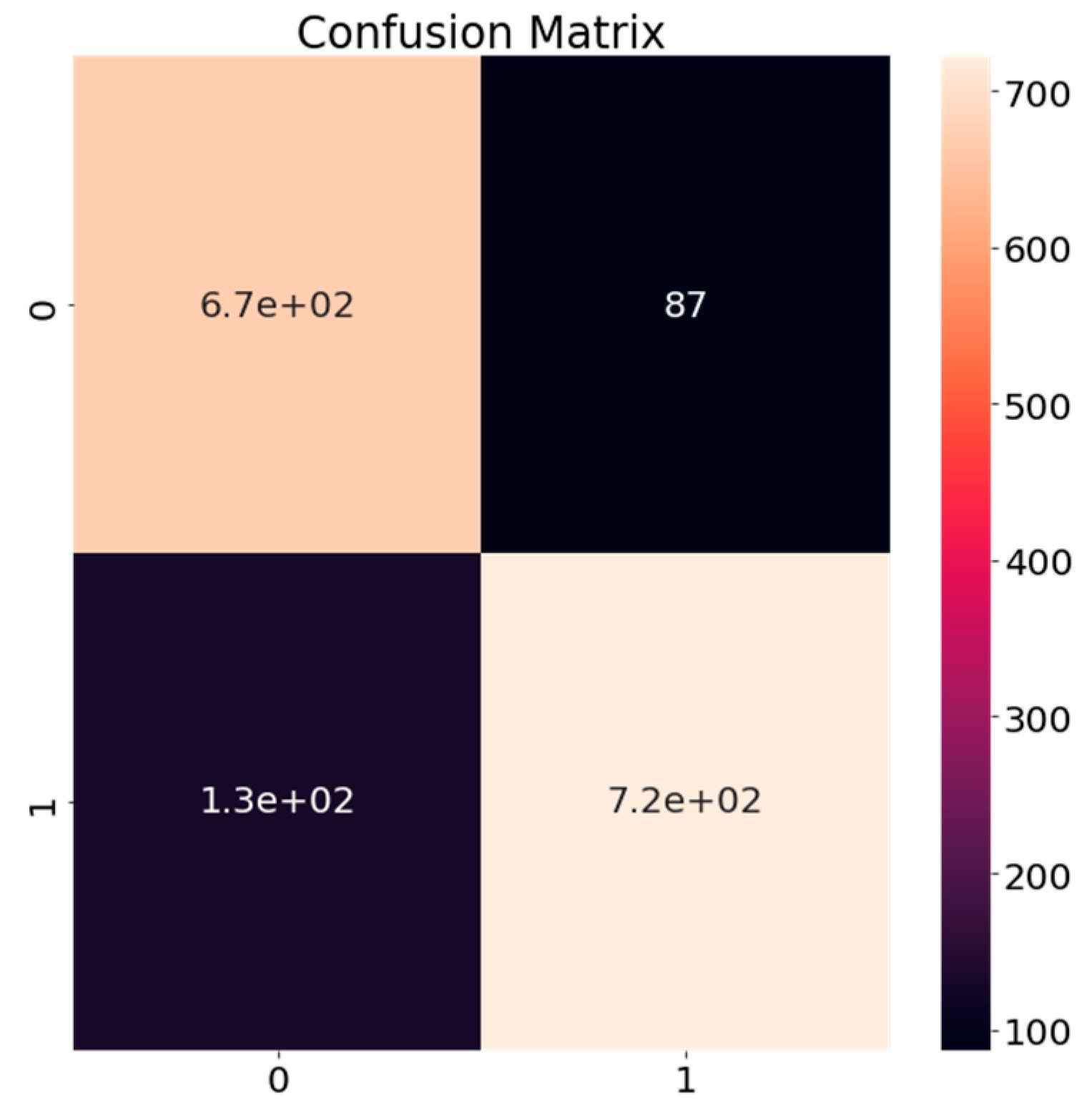
The DNN classification model’s confusion matrix is shown in Figure 11. By definition, in a confusion matrix C, the number of observations that are both known to belong to group i and expected to belong to group j is equal to Ci,j. Therefore, in a binary classification, the counts of true negatives, false negatives, true positives, and false positives are C0, 0, C1, 0, and C0, respectively. Since we found that the false negatives were only C1,0 = 87 and that the false positives were C0,1 = 132, which translates to an accuracy value of 0.87, our model demonstrated a highly acceptable classification performance, given the large variability of our target value (). In other words, 87% of the model’s predictions were correct.
5. Conclusions
This paper was comprised of two parts, which presented a thorough analysis of modeling and strength-level classification by leveraging machine-learning algorithms.
The first part presented the analysis of regression modeling. Four common ML algorithms were utilized and trained on a preliminary dataset consisting of six experimentally obtained macroscopic meteorological parameters. The results showed very good prediction accuracy for every model. Specifically, the ANN algorithm, a single-layer-perceptron model that included 70 neurons in its hidden layer, with a training-batch size of 32, trained with a Levenberg–Marquardt algorithm, resulted in an R-squared of 0.896 and a mean square error (MSE) of 0.0834. The RF algorithm, comprising 80 estimators, also gave a highly acceptable coefficient of determination, an R-squared of 0.865, and a root mean square error (RMSE) of 0.241. The gradient boosting regressor model, with 1000 boosting stages (n_estimators), a learning rate of 0.05, a maximum depth of individual regression estimators equal to six, and a minimum number of samples required to split an internal node equal to twelve, resulted in an R-squared of 0.851 and a root-mean-square error (RMSE) of 0.252. Finally, the DNN algorithm, comprising three hidden layers of neurons (first hidden layer = 30, second hidden layer = 20, and third hidden layer = 10), run over batches of 16 for a total number of 350 epochs, resulted in R2 = 0.79 and RMSE = 0.088.
The second part described a DNN approach to classify the turbulence-strength level as either strong or weak utilizing the same data set. A notional value of the refractive-index structural parameter, , was set to distinguish between the strong and weak regions, and the resulting split of the experimental data was quite balanced. The network had three hidden layers with 30, 20, and 10 neurons, respectively, and a dropout rate of 0.5 per layer. The algorithm was trained against 80% of the dataset and tested over the remaining 20%, for a total number of 500 training epochs and a batch size of 8. The model exhibited a very acceptable classification performance, given the highly variability of our target value (), since we observed an accuracy of 87% in the predictions made by the model.
Author Contributions
A.L.: conceptualization, methodology, software, validation, data curation, writing—draft; K.P.: software, formal analysis, review, editing, supervision, project administration; H.E.N.: formal analysis, review, editing, supervision, project administration; A.T.: formal analysis, review, editing, resources, supervision, project administration; K.C.: software, formal analysis, review, editing, supervision; K.R.D.: methodology, formal analysis, review. All authors have read and agreed to the published version of the manuscript.
Funding
This research did not receive any specific grant from funding agencies in the public, commercial, or not-for-profit sectors.
Data Availability Statement
Data unavailable due to privacy restrictions.
Conflicts of Interest
The authors declare no conflict of interest.
References
- Khalingi, M.A.; Uysal, M. Survey on Free Space Optical Communication: A Communications Theory Perspective. IEEE Commun. Surv. Tutor. 2014, 16, 2231–2258. [Google Scholar]
- Doss-Hammel, S.; Tsindikidis, D.; Merritt, D.; Fontana, J. Atmospheric characterization for high energy laser beam propagation in the maritime environment. In Atmospheric Tracking, Imaging and Compensation, Proceedings of the SPIE 49th Annual Meeting, Denver, CO, USA, 2–6 August 2004; Valley, M.T., Vorontsov, M., Eds.; SPIE: Bellingham, WA, USA, 2004. [Google Scholar]
- Lionis, A.; Peppas, K.; Nistazakis, H.E.; Tsigopoulos, A.D.; Cohn, K. Experimental Performance Analysis of an Optical Communication Channel over Maritime Environment. Electronics 2020, 9, 1109. [Google Scholar] [CrossRef]
- Lionis, A.; Peppas, K.; Nistazakis, H.E.; Tsigopoulos, A.D.; Cohn, K. Statistical Modeling of Received Signal Strength for an FSO Channel over Maritime Environment. Opt. Commun. 2021, 489, 126858. [Google Scholar] [CrossRef]
- Lionis, A.; Peppas, K.; Nistazakis, E.; Tsigkopoulos, A.; Cohn, K. RSSI probability density functions comparison using Jenshen-Shannon divergence and Pearson distribution. Technologies 2021, 9, 26. [Google Scholar] [CrossRef]
- Lionis, A.; Chaskakis, G.; Cohn, K.; Blau, J.; Peppas, K.; Nistazakis, H.E.; Tsigopoulos, A. Optical Turbulence Measurements and Modeling over Monterey Bay. Opt. Commun. J. 2022, 520, 128508. [Google Scholar] [CrossRef]
- Majumdar, A.K. Free-space laser communication performance in the atmospheric channel. J. Opt. Fiber Commun. 2005, 2, 345–396. [Google Scholar] [CrossRef]
- Sabot, D.; Kopeika, N.S. Forecasting optical turbulence strength on the basis of macroscale meteorology and aerosols: Models and validation. Opt. Eng. 1992, 31. [Google Scholar] [CrossRef]
- Oermann, R.J. Novel Methods for the Quantification of Atmospheric Turbulence Strength in the Atmospheric Surface Layer. Ph.D. Thesis, School of Chemistry and Physics, University of Adelaide, Adelaide, SA, Australia, 2014. [Google Scholar]
- Lionis, A.; Tsigopoulos, A.; Keith, C. An Application of Artificial Neural Networks to Estimate the Performance of High-Energy Laser Weapons in Maritime Environments. Technologies 2022, 10, 71. [Google Scholar] [CrossRef]
- Frederickson, P.A.; Davidson, K.L.; Zeisse, C.R.; Bendall, C.S. Estimating the refractive index structure parameter (Cn2) over the ocean using bulk methods. J. Appl. Meteorol. 2000, 39, 1770–1783. [Google Scholar] [CrossRef]
- Frederickson, P.; Hammel, S.; Tsintikidis, D. Measurements and modeling of optical turbulence in a maritime environment. In Proceedings of the SPIE Optics + Photonics, San Diego, CA, USA, 13–17 August 2006. [Google Scholar] [CrossRef]
- Moore, C.I.; Burris, H.R.; Stell, M.F.; Wasiczko, L.; Suite, M.R.; Mahon, R.; Rabinovich, W.S.; Gilbreath, G.C.; Scharpf, W.J. Atmospheric turbulence studies of a 16-km maritime path. In Proceedings of the SPIE 5793, Atmospheric Propagation II, Orlando, FL, USA, 25 May 2005. [Google Scholar]
- Burris, H.R.; Moore, C.I.; Swingen, L.A.; Vilcheck, M.J.; Tulchinsky, D.A.; Mahon, R.; Wasiczko, L.M.; Stell, M.F.; Suite, M.R.; Davis, M.A.; et al. Latest Results from the 32 km Maritime Lasercom Link at the Naval Research Laboratory, Chesapeake Bay Lasercom Test Facility. In Proceedings of the SPIE 5793, Atmospheric Propagation II, Orlando, FL, USA, 28 March–1 April 2005. [Google Scholar] [CrossRef]
- Wasiczko, L.M.; Moore, C.I.; Burris, H.R.; Suite, M.; Stell, M.; Murphy, J.; Gilbreath, G.C.; Rabinovich, W.; Scharpf, W. Characterization of the Marine Atmosphere for Free-Space Optical Communication. In Proceedings of the SPIE 6215, Atmospheric Propagation III, Orlando, FL, USA, 17 May 2006. [Google Scholar]
- Gilbreath, G.C.; Rabinovich, W.S.; Moore, C.I.; Burris, H.R.; Mahon, R.; Grant, K.J.; Goetz, P.G.; Murphy, J.L.; Suite, M.R.; Stell, M.F.; et al. Progress in Laser Propagation in a Maritime Environment at the Naval Research Laboratory. In Proceedings of the SPIE 5892, Free-Space Laser Communications V, San Diego, CA, USA, 31 July–4 August 2005. [Google Scholar] [CrossRef]
- Grant, K.J.; Mudge, K.A.; Clare, B.A.; Perejma, A.S.; Martinsen, W.M. Maritime Laser Communications Trial 98152-19703. In Command, Control, Communications and Intelligence Division; DSTO: Edinburgh, SA, Australia, 2012. [Google Scholar]
- Michael, S.; Parenti, R.R.; Walther, F.G.; Volpicelli, A.M.; Moores, J.D.; Wilcox, W., Jr.; Murphy, R. Comparison of Scintillation Measurements from a 5 km Communications Link to Standard Statistical Models. In Proceedings of the SPIE 7324, Atmospheric Propagation VI, Orlando, FL, USA, 2 May 2009. [Google Scholar]
- Jang, Y.; Ma, J.; Tan, L.; Yan, S.; Du, W. Measurement of optical intensity fluctuation over an 11.8 km turbulent path. Opt. Express 2008, 16, 6963–6973. [Google Scholar] [CrossRef]
- Ali, R.N.; Jassim, J.M.; Jasim, K.M.; Jawad, M.K. Experimental Study of Clear Atmospheric Turbulence Effects on Laser Beam Spreading in Free Space. Int. J. Appl. Eng. Res. 2017, 12, 14789–14796. [Google Scholar]
- Pan, F.; Han, Q.; Ma, J.; Tan, L. Measurement of scintillation and link margin for laser beam propagation on 3.5-km urbanised path. Chin. Opt. Lett. 2007, 5, 1–3. [Google Scholar]
- Libich, J.; Komanec, M.; Zvanovec, S.; Pesek, P.; Popoola, W.O.; Ghassemlooy, Z. Experimental verification of an all-optical dual-hop 10 Gbit/s free-space optics link under turbulence regimes. Opt. Lett. 2015, 40, 391–394. [Google Scholar] [CrossRef]
- Tunick, A. Statistical analysis of optical turbulence intensity over a 2.33 km propagation path. Opt. Express 2007, 15, 3619–3628. [Google Scholar] [CrossRef]
- van de Boer, A.; Moene, A.F.; Graf, A.; Simmer, C.; Holtslag, A.A.M. Estimation of the refractive index structure parameter from single-level daytime routine weather. Appl. Opt. 2014, 53, 5944–5960. [Google Scholar] [PubMed]
- James, G.; Witten, D.; Hastie, T.; Tibshirani, R. An Introduction to Statistical Learning with Applications in R; Springer: New York, NY, USA; Berlin/Heidelberg, Germany; Dordrecht, The Netherlands; London, UK, 2013. [Google Scholar]
- Brownlee, J. Better Deep Learning: Train Faster, Reduce Overfitting, and Make Better Predictions; Machine Learning Mastery: Victoria, Australia, 2018. [Google Scholar]
- Kim, P. MATLAB Deep Learning: With Machine Learning, Neural Networks and Artificial Intelligence; Springer Science+Business Media: New York, NY, USA, 2017. [Google Scholar] [CrossRef]
- Wang, D.; Song, Y.; Li, J.; Qin, J.; Yang, T.; Zhang, M.; Chen, X.; Boucouvalas, A. Data-driven Optical Fiber Channel Modeling: A Deep Learning Approach. J. Light. Technol. 2020, 38, 4730–4743. [Google Scholar] [CrossRef]
- Liu, J.; Wang, P.; Zhang, X.; He, Y.; Zhou, X.; Ye, H.; Li, Y.; Xu, S.; Chen, S.; Fan, D. Deep learning based atmospheric turbulence compensation for orbital angular momentum beam distortion and communication. Opt. Express 2019, 27, 16671–16688. [Google Scholar] [PubMed]
- Amirabadi, M.; Kahaei, M.; Nezamalhosseini, S.A.; Vakili, V.T. Deep Learning for channel estimation in FSO communication system. Opt. Commun. 2020, 459, 124989. [Google Scholar] [CrossRef]
- Lohani, S.; Glasser, R. Turbulence correction with artificial neural networks. Opt. Lett. 2018, 43, 2611–2614. [Google Scholar] [CrossRef]
- SLohani; Knutson, E.M.; Glasser, R.T. Generative machine learning for robust free-space communication. Commun. Phys. 2020, 3, 177. [Google Scholar] [CrossRef]
- Mishra, P.; Sonali; Dixit, A.; Jain, V.K. Machine Learning Techniques for Channel Estimation in Free Space Optical Communication Systems. In Proceedings of the 2019 IEEE International Conference on Advanced Networks and Telecommunications Systems (ANTS), GOA, India, 16–19 December 2019; pp. 1–6. [Google Scholar] [CrossRef]
- Jellen, C.; Burkhardt, J.; Brownell, C.; Nelson, C. Machine learning informed predictor importance measures of environmental parameters in maritime optical turbulence. Appl. Opt. 2020, 59, 6379–6389. [Google Scholar] [CrossRef] [PubMed]
- Wang, Y.; Basu, S. Using an artificial neural network approach to estimate surface-layer optical turbulence at Mauna Loa, Hawaii. Opt. Lett. 2016, 41, 2334–2337. [Google Scholar] [CrossRef] [PubMed]
- Lionis, A.; Peppas, K.; Nistazakis, H.E.; Tsigopoulos, A.; Cohn, K.; Zagouras, A. Using Machine Learning Algorithms for Accurate Received Optical Power Prediction of an FSO Link over a Maritime Environment. Photonics 2021, 8, 212. [Google Scholar] [CrossRef]
- Lionis, A.; Sklavounos, A.; Stassinakis, A.; Cohn, K.; Tsigopoulos, A.; Peppas, K.; Aidinis, K.; Nistazakis, H. Experimental Machine Learning Approach for Optical Turbulence and FSO Outage Performance Modeling. Electronics 2023, 12, 506. [Google Scholar] [CrossRef]
- Available online: https://weather-stats.com/greece/athenes/sea_temperature#details (accessed on 1 June 2022).
- Kaushal, H.; Jain, V.K.; Kar, S. Free Space Optical Communication, Optical Networks; Springer: New Delhi, India, 2017. [Google Scholar] [CrossRef]
Figure 1.
The laser-communications link located across the entrance to Piraeus port.

Figure 2.
The MRV TS5000/155 FSO system, co-located with the BLS450 scintillometer and the ambient-weather WS-2000 weather station on the roof of the laboratory building of the Hellenic Naval Academy.
Figure 2.
The MRV TS5000/155 FSO system, co-located with the BLS450 scintillometer and the ambient-weather WS-2000 weather station on the roof of the laboratory building of the Hellenic Naval Academy.

Figure 3.
Regression plot for the single-hidden-layer network.

Figure 4.
Scatter plot (left) and line plot (right) for observed vs. predicted values for the random forest regression model.
Figure 4.
Scatter plot (left) and line plot (right) for observed vs. predicted values for the random forest regression model.

Figure 5.
Scatter plot (left) and line plot (right) for observed vs. predicted values for the gradient boosting regression model.
Figure 5.
Scatter plot (left) and line plot (right) for observed vs. predicted values for the gradient boosting regression model.

Figure 6.
Τhe line plot of the loss function during DNN-model training.

Figure 7.
Scatter plot (left) and line plot (right) for observed vs. predicted values for the DNN regression model.
Figure 7.
Scatter plot (left) and line plot (right) for observed vs. predicted values for the DNN regression model.

Figure 8.
The three-layer deep neural network for turbulence-strength classification.

Figure 9.
The cumulative results of the turbulence-strength level. The “0” denotes weak and “1” denotes strong turbulence conditions.
Figure 9.
The cumulative results of the turbulence-strength level. The “0” denotes weak and “1” denotes strong turbulence conditions.

Figure 10.
The loss/accuracy performance of the deep neural classifier of the turbulence strength for a total of 500 epochs.
Figure 10.
The loss/accuracy performance of the deep neural classifier of the turbulence strength for a total of 500 epochs.

Figure 11.
The confusion matrix for the DNN classifier.

Disclaimer/Publisher’s Note: The statements, opinions and data contained in all publications are solely those of the individual author(s) and contributor(s) and not of MDPI and/or the editor(s). MDPI and/or the editor(s) disclaim responsibility for any injury to people or property resulting from any ideas, methods, instructions or products referred to in the content. |
© 2023 by the authors. Licensee MDPI, Basel, Switzerland. This article is an open access article distributed under the terms and conditions of the Creative Commons Attribution (CC BY) license (https://creativecommons.org/licenses/by/4.0/).
Share and Cite
MDPI and ACS Style
Lionis, A.; Peppas, K.; Nistazakis, H.E.; Tsigopoulos, A.; Cohn, K.; Drexler, K.R. Supervised Machine Learning for Refractive Index Structure Parameter Modeling. Quantum Beam Sci. 2023, 7, 18. https://doi.org/10.3390/qubs7020018
AMA Style
Lionis A, Peppas K, Nistazakis HE, Tsigopoulos A, Cohn K, Drexler KR. Supervised Machine Learning for Refractive Index Structure Parameter Modeling. Quantum Beam Science. 2023; 7(2):18. https://doi.org/10.3390/qubs7020018
Chicago/Turabian StyleLionis, Antonios, Konstantinos Peppas, Hector E. Nistazakis, Andreas Tsigopoulos, Keith Cohn, and Kyle R. Drexler. 2023. "Supervised Machine Learning for Refractive Index Structure Parameter Modeling" Quantum Beam Science 7, no. 2: 18. https://doi.org/10.3390/qubs7020018