Article

SAR Interferometry Data Exploitation for Infrastructure Monitoring Using GIS Application

1
Department of Civil, Building and Environmental Engineering (DICEA), Sapienza University of Rome, 00184 Rome, Italy
2
Survey Lab, Spin-off-Sapienza University of Rome, 00184 Rome, Italy
*
Author to whom correspondence should be addressed.
Infrastructures 2023, 8(5), 94; https://doi.org/10.3390/infrastructures8050094
Submission received: 12 March 2023 / Revised: 13 April 2023 / Accepted: 12 May 2023 / Published: 16 May 2023

Abstract

:
Monitoring structural stability in urban areas and infrastructure networks is emerging as one of the dominant socio-economic issues for population security. The problem is accentuated by the age of the infrastructure because of increasing risks due to material deterioration and loss of load capacity. In this case, SAR satellite data are crucial to identify and assess the deteriorating conditions of civil infrastructures. The large amount of data available from SAR satellite sensors leads to the exploitation and development of new GIS-based procedures for rapid responses and decision making. In recent decades, the DInSAR technique has been used efficiently for the monitoring of structures, providing measurement points located on structures with millimeter precision. Our study has analyzed the behavior of structures in settlements, attempting to discuss the interactions of soil and structures, and examining the behavior of different types of structures, such as roads and buildings. The method used is based on long-term SAR interferometry data and a semi-automatic procedure to measure the displacement (mm/year) of structures, through a GIS-based application performed in the “Implemented MOnitoring DIsplacement” I.MODI platform. The analysis provides extensive information on long-term spatial and temporal continuity of up to 25 years of record, using satellite SAR multi-sensors from ERS, Envisat, and COSMO-SkyMed. The interpretation uses time series spatial analysis, supported by orthophotos, and layers of the DBTR (regional topographic database), Digital Surface model (DSM), and hydrogeological map to show anomalous areas with a high displacement rate and to observe the correlation of settlements in the sediments. With the satellite information and Geographic Information System (GIS), we were able to observe relevant parameters, such as the velocity of advance in the direction of the slope (deformation profiles), the cumulative displacement, and the trend changes in structures. The results illustrate an innovative procedure that allows the management of DInSAR data to facilitate the effective management of structures in which a monitoring protocol was developed at different spatial scales, integrating the information into a GIS.

Graphical Abstract

1. Introduction

Structural monitoring due to anthropic transformation of the natural environment is a key factor in mitigating risks to structures and the surrounding environment [1,2]. The quantitative assessment of displacements that affect structures is traditionally based on ground instrumentation, such as leveling, automatic total station, and laser scanners. A number of methods for in situ and remote data collection are available with the aim of monitoring both the evolution of natural and anthropogenic ground deformation processes and the degradation of construction materials of structural components of civil engineering structures [3,4]. However, these techniques require long survey times for the installation of instruments and targets on the structures to collect accurate and reliable measurements [5,6].
Among non-invasive structural monitoring techniques, Differential Interferometry Synthetic Aperture Radar (DInSAR) can provide useful information to support process management and security assessments, thereby reducing the risk of building/infrastructure functionality [7]. In particular, ground displacement velocity maps (mm/year) and time series based on advanced multi-temporal DInSAR technology, combined with land registers and geological information, can be of great help for timely structural assessments.
In recent years, numerous DInSAR studies have been carried out to monitor soil deformation induced by natural and/or anthropogenic processes. Among others, different studies have assessed ground instabilities. Bianchini et al. [8] developed a methodology to evaluate the stability of buildings affected by landslide phenomena based on two parameters derived from the deformation rates derived from measurement points (maximum differential settlement and angular distortion). Scifoni et al. [9] used a joint approach of spatial technology with geological information to study the structural behavior of the urban center area of Rome (Italy). Arangio et al. [10] and Peduto et al. [11] used the DInSAR technique to determine the structural damage of buildings complemented with structural modeling. Many studies have been conducted using DInSAR in the field of monitoring individual infrastructures, such as bridges, e.g., [12,13], railways, e.g., [14,15], and crossrails, e.g., [16,17,18]. Studies have also used DInSAR for the monitoring of infrastructure networks [19,20,21]. On the other hand, GIS-based procedures from DInSAR data have been used for decision making in different contexts, for urban areas, e.g., [22], volcanic scenarios, e.g., [23], landslides, e.g., [24], and mining applications, e.g., [25]. Unlike these studies, this research presents an innovative procedure used as a monitoring tool, based on the implementation of GIS catalogs, which clearly supports the effectiveness of the use of SAR data and land registers for maintenance and decision making.
DInSAR is based on the exploitation of the phase difference (interferogram) between two SAR images, recording information in the Line-Of-Sight (LOS) projection of the sensor of the detected displacements that occurred between the two acquisition times [9]. The use of advanced DInSAR approaches [26,27,28,29,30], based on the exploitation of large sets of multitemporal SAR data, makes it possible to provide useful information on the spatial and temporal patterns of movements detected through the generation of time series [31,32,33], allowing the identification of geohazards due to natural or anthropogenic phenomena and their implications in infrastructures [34,35]. DInSAR’s capability of effectively extracting reliable measures from the large amount of data available in the satellite images of space agencies and from the data collected by the new sensors at a greater frequency and resolution make it an attractive solution [36]. The availability of DInSAR open data, the large amount of interferometric data available on a national scale from the Italian remote sensing non-ordinary plan [37], and the Ground Motion Service project on a continental scale has become increasingly accessible [38]. The ESA (European Space Agency) makes data acquired from the main SAR satellites available. Therefore, the development of new applications is essential for the management and distribution of timely information for infrastructure monitoring.
Structural health monitoring can be verified with the geometry of the building provided by the land registers and the spatial coverage of the DInSAR data, providing useful information for the behavior of the structure at measurement point locations. Therefore, it is possible to understand the static behavior of individual structures through displacement time series analysis [39]. It is worth mentioning that DInSAR can detect near-vertical deformations along the Line-Of-Sight (LOS) of the satellite’s SAR sensor with millimeter accuracy.
In this research scenario, the work focuses on the structural monitoring of buildings and roads affected by settlements, exploiting DInSAR data into GIS-based mapping for long-term monitoring (15 to 25 years). In particular, processing has been carried out by applying the advanced DInSAR technique called Small Baseline Subset (SBAS) [27,29] to a set of SAR data from the ERS, Envisat, and COSMO-SkyMed satellites. The SBAS approach is based on the proper selection of a large number of SAR data pairs. These pairs are used to generate small baseline differential interferograms to mitigate noise (i.e., decorrelation phenomena) affecting interferograms and to maximize the number of reliable measurement points. Deformation time series are computed by searching for a least-squares solution with a minimum standard energy constraint (the SVD technique is applied in the presence of different subsets of data separated by large baselines) [31]. For each coherent measurement point, the displacement time series and mean strain rate are retrieved with millimeter precision [33,40].
GIS procedures and spatial analysis techniques have been adopted to extract patterns in anomalous structures and reconstruct long periods of settlement, estimating parameters, such as velocity of displacement (mm/year), cumulative displacements [mm], deformation profiles, and analysis of time series. The GIS-based classification proposes to systematize the capacities and technologies of its structures that operate in the civil engineering sectors through mapping and detection of anomalies in civil infrastructures. It is intended to determine a flexible and adaptable approach to the different categories of buildings and roads, which, due to their functionality, encompass different works in environmental and geological contexts. In order to interpret the typical subsidence process, the study area of Rome is proposed, where settlement is related to external loads due to recent urbanization and the local geological and geotechnical environment determined by highly compressible alluvial and coastal deposits. The interpretation of the results is based on historical cartography, such as orthophotos, and details of hydrogeological maps, as well as topographic data from Light Detection and Ranging (LiDAR) and high resolution Digital Surface Models (DSM). The results of the study can be applied for territorial planning and risk management purposes. In addition, the peculiar geological environment and the strategic importance of the area make them of interest to the scientific community.

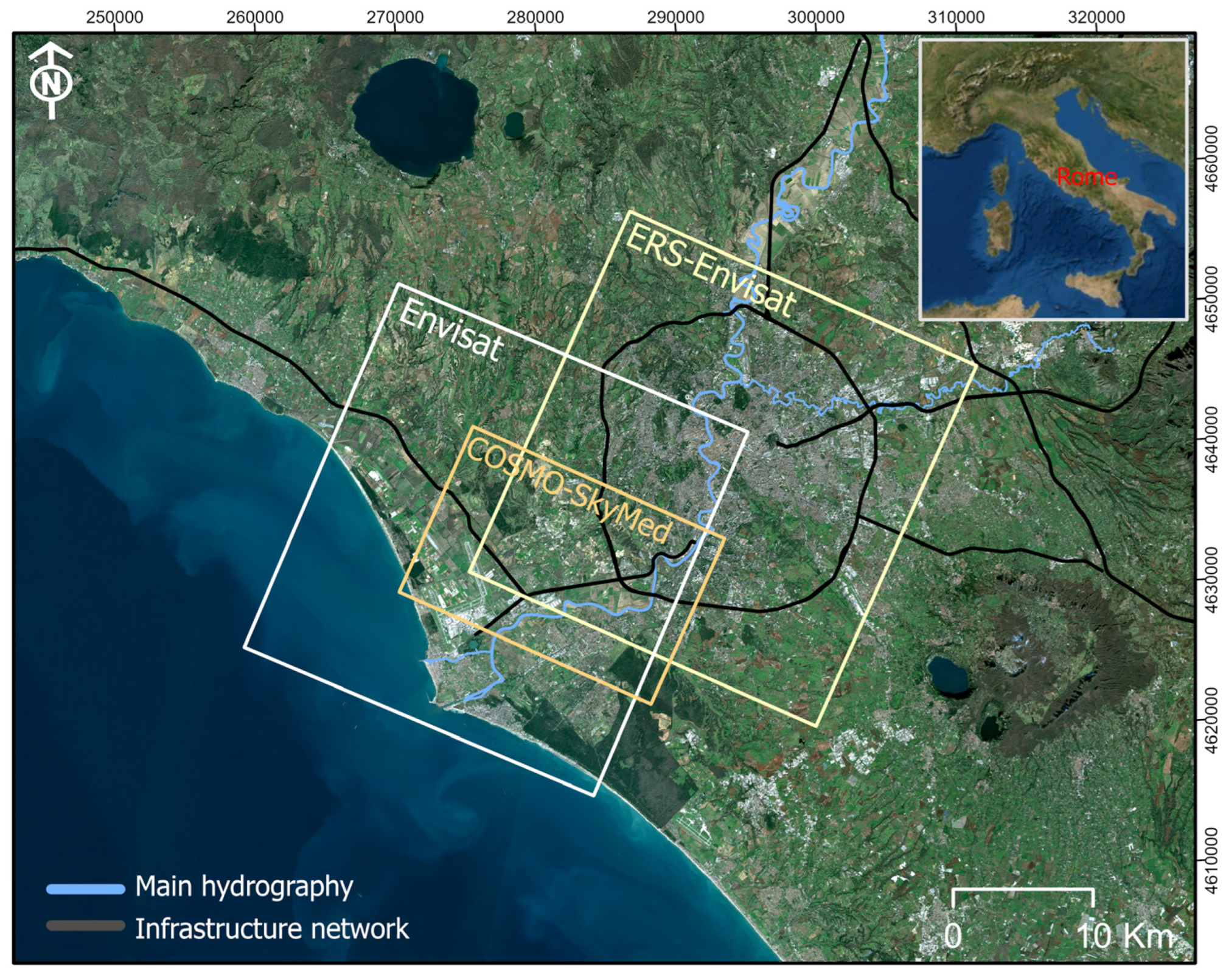
2. Study Area, Hydrogeological Context, and Infrastructure Network

2.1. Hydrogeological Context

As already mentioned, the investigated region is the city of Rome and its surroundings. This city has a historical connection with water; its large aqueducts, fountains, rivers, and the sea have defined the characteristics of its environment. The Tiber delta has been interpreted as dominated by waves [41,42]. The hydrogeological characterization for this work is the Hydrogeological Map of the City of Rome, scale 1:50,000 prepared by La Vigna et al. [43], which is shown in Figure 1.
Hydrogeological formations have been defined in hydrogeological complexes, each characterized by the same transmission and storage capacities, as well as for a similar hydrogeological significance with respect to groundwater circulation at the scale of the entire study area [44,45]. The hydrogeological environment of the Tiber area has a deep and artesian main aquifer located in sand gravel; it is supported at the base by clays from the lower Pleistocene that act as an aquifer and at the top partially sealed by deposits of clay and limestone with low permeability [46]. Another aquifer is found in sandy deposits; its piezometry has been reconstructed to the left of the Tiber River [47,48]. The piezometric distribution shows that the upper part of the aquifer is below sea level in most regions. The maximum depression is just south of ancient Ostia, with altitudes reaching 5 m above sea level. These values are related to the increase in the use of pumping wells associated with an increase in urbanization [47,48].
The Tiber delta covers a total area of approximately 2000 ha. On a large scale, proceeding from the coast toward the interior, the A91 Highway runs over deposits dated to different Quaternary depositional environments: deltaic and coastal deposits are present for a width of about 5–40 km from the coast line (from a sandy to pelitic lithofacies), covering Area 1 and Area 2. Recent and current alluvial deposits constitute a hydrogeological unit on the Hydrogeological Map of Rome, belonging to the ancient areas of the Tiber lagoon delta during the Transgressive Sequence Tract (TST) phase [41] and consisting of fossiliferous pelitic sediments and alluvial deposits developed from a recent floodplain, superimposed on deposits belonging to a fluvial apparatus with interlocking channels covered with locally sandy and clayey silts.

2.2. Infrastructure Network

The infrastructure network is located in the Tiber Delta, in the Rome metropolitan area, and in the Lazio region, Italy, where structures are exposed to highly compressible alluvial soils around the A91 and GRA Highways. The area is also characterized by the coexistence of transport infrastructures, concentrated in an environment of high logistical and commercial value; specifically, the study area represents a strategic sector at a national and international level, connecting the Leonardo Da Vinci International Airport and the port of Ostia. The landscape of this area is defined by the Tiber River, with a mainly curved watercourse in the Rome-Fiumicino area and an average flow of 320 m³/s.
Two test areas, Area 1 (A1) and Area 2 (A2), were selected with the use of orthophotos, and it was possible to reconstruct an evolutionary period of urbanization for A1 and area A2 (see Figure 2), described below:
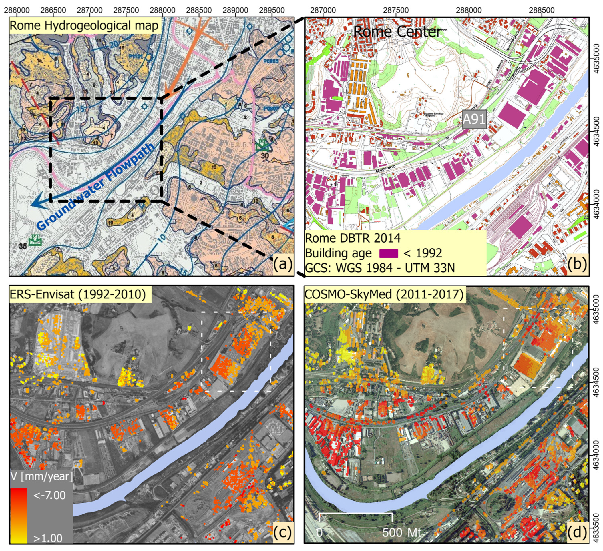
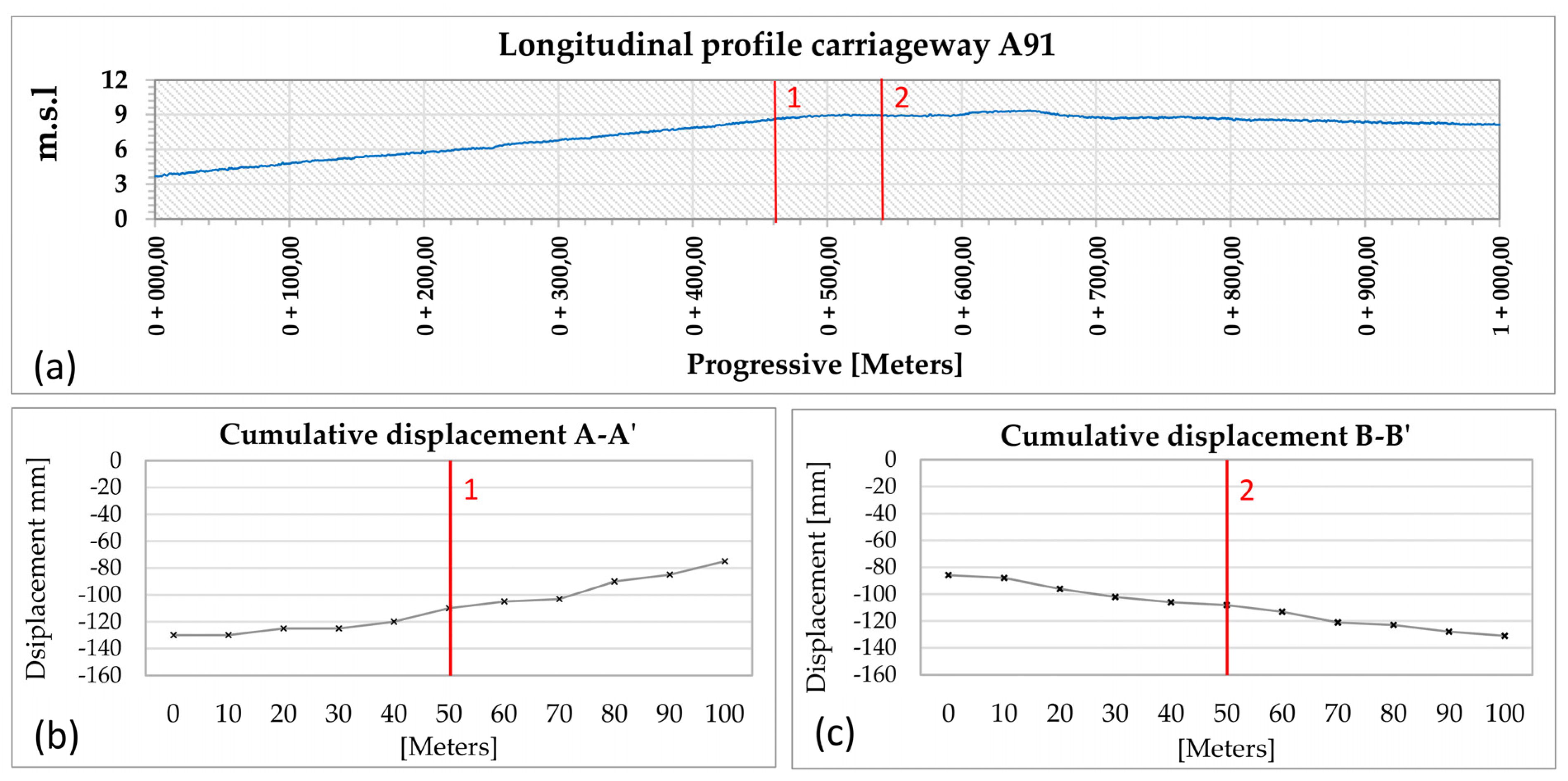
  • Area 1: Located in the center of Rome in the Tiber River valley, it does not show important changes in urbanization; therefore, the SAR observation on the A1 infrastructures have been continuous since 1992.
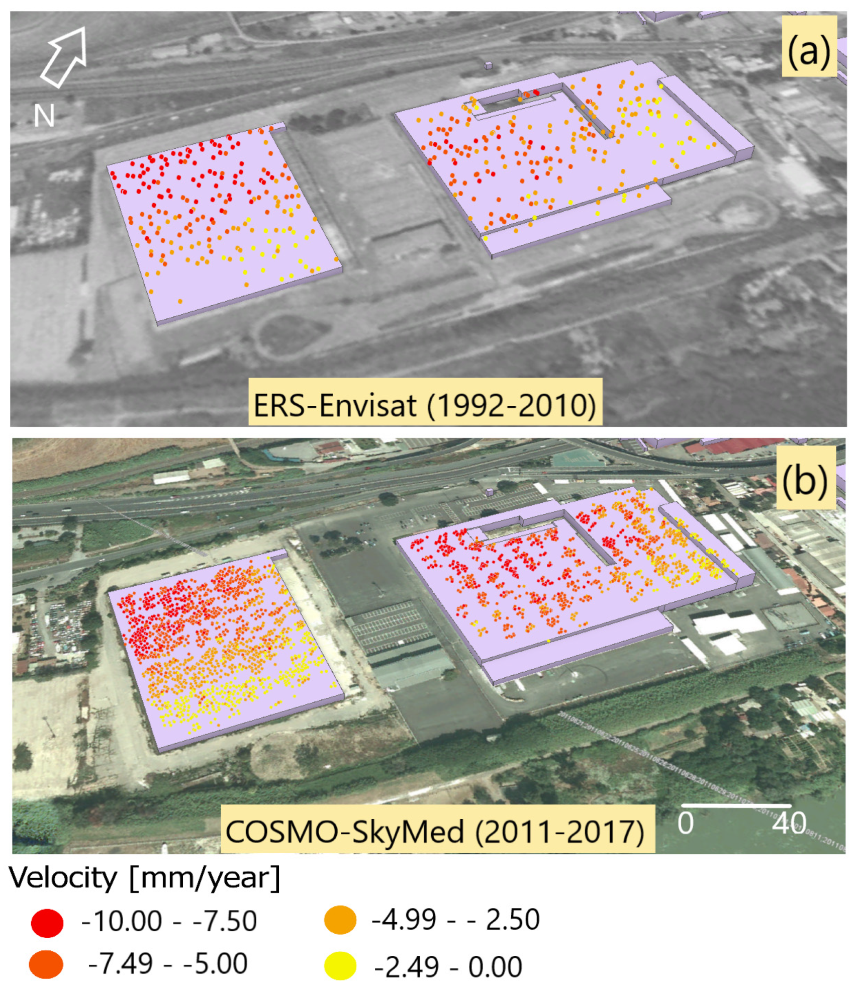
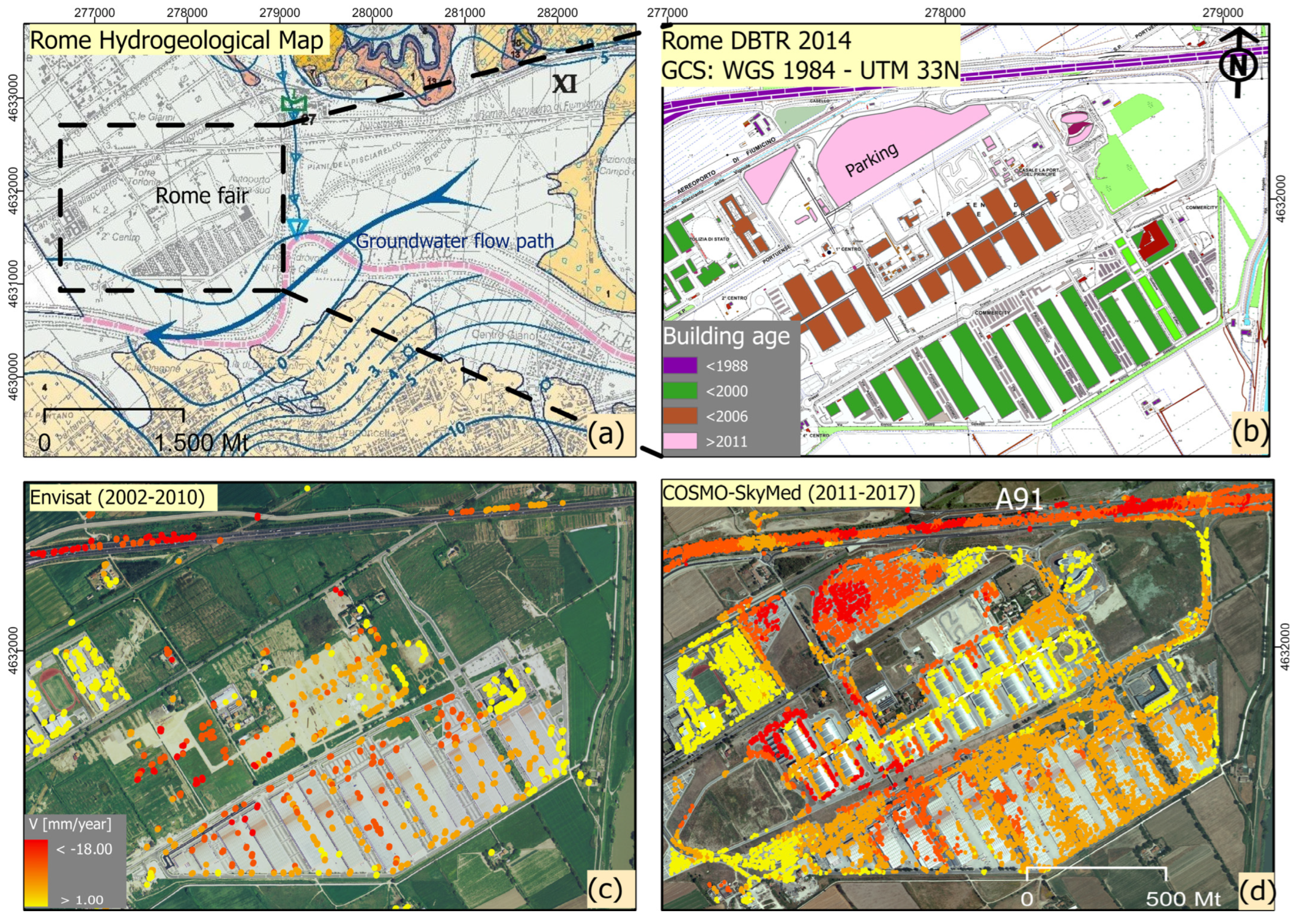
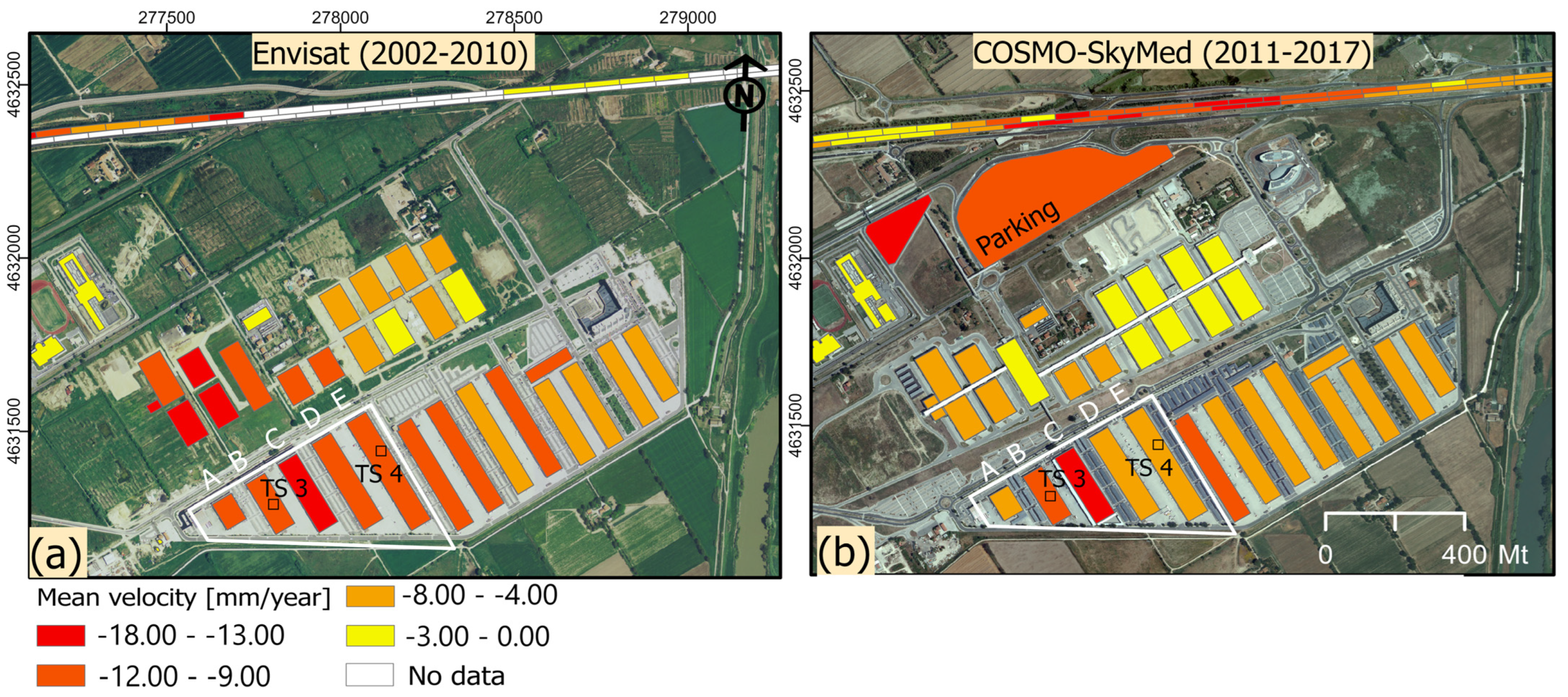
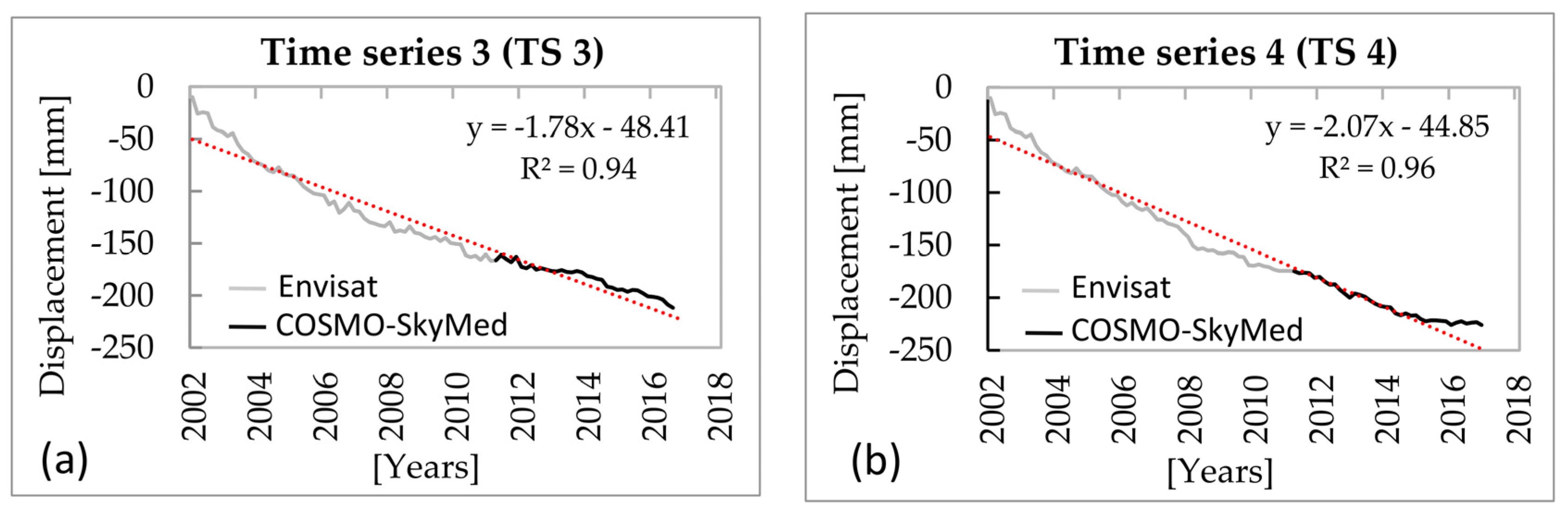
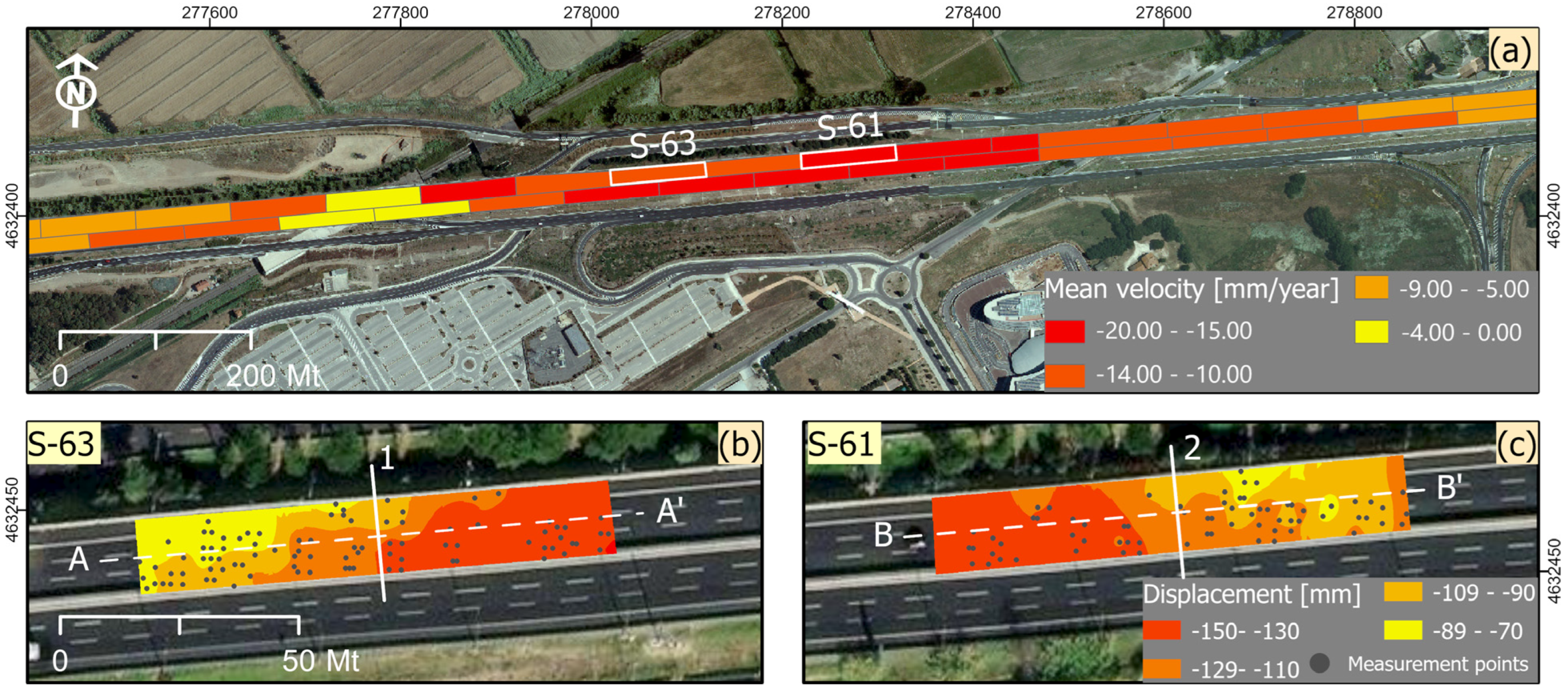
  • Area 2: Located in the Tiber River delta, there is an increase in urbanization and important changes, mainly new constructions in the logistics and commercial field, such as the Rome fair, and service infrastructure, such as parking lots, carried out between 2006 and 2011. Unlike the A91 Highway built in 1959.

3. Materials and Methods

The methodology proposes a workflow based on the integration of DInSAR remote measurements and the Geographic Information System (GIS) for the generation of catalogs through a GIS-mapping semi-automatic procedure.
The method uses DInSAR data from the Small BAseline Subset (SBAS) technique and the GIS platform. For the interpretation of the SAR sensor measurements, optical and technical cartography, Digital Surface Model (DSM), and hydrogeological characterization have been used. The GIS application procedure is implemented in two test areas, Area 1 (A1) and Area 2 (A2), following three main steps, described in: Section 3.1 Data collection, Section 3.2 SAR image processing, and Section 3.3 GIS mapping.

3.1. Data Collection

In order to classify the measurement points and associate them with the deformation phenomena that affect the structures, a dataset was collected, mainly GIS vector data, such as polygons of buildings and roads, from the Regional Topographic Database (DBTR) (see Figure 3). In addition, orthophotos were used as the base cartography, Digital Surface Model (DSM) from LiDAR-1mt resolution as topography and georeferencing of measurement point data, and hydrogeological information for settlement interpretation; all datasets are described in Table 1.

3.2. SAR Image Processing
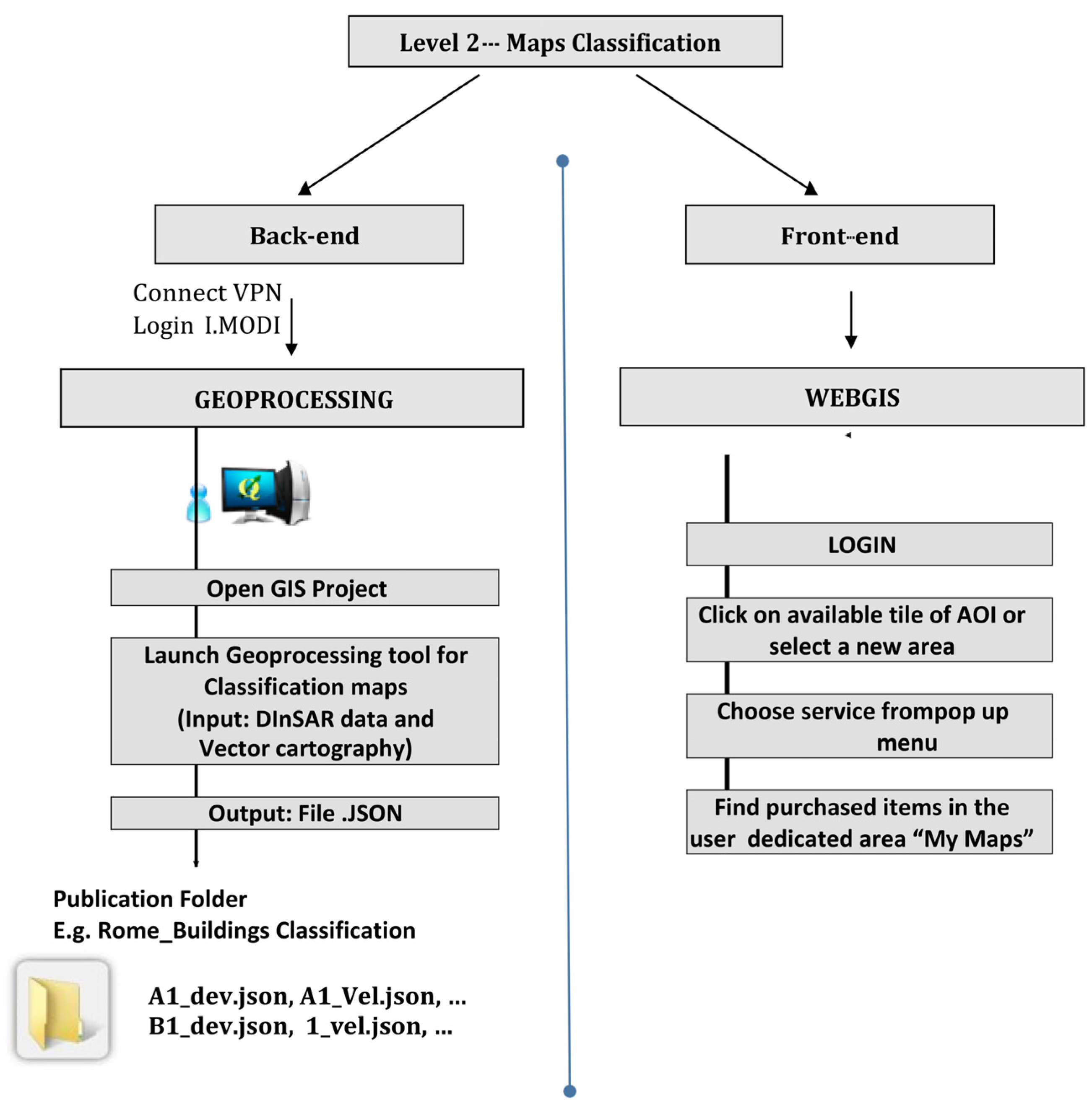
The SBAS-DInSAR multitemporal technique [27,29] allows mapping of the movements of the structures, generating average strain rate maps and time series. The approach is based on an adequate selection of a large number of SAR image pairs, with short spatial and temporal separations (baseline), in order to mitigate decorrelation phenomena [49] and maximize the number of reliable images through SAR measurement. The measurement points recorded by the DInSAR technique are called SBAS (Small Baseline Subset), which allows the identification of natural (such as exposed rocks) or artificial (such as buildings and metal structures) targets on the ground. Using DInSAR observations, it is possible to measure the displacement in time along the Line-Of-Sight (LOS) with respect to a “reference point” considered stable within the “frame”, corresponding to the satellite observation range.
The measurement points adopted from SBAS are used in urban areas or at least where the targets remain stable in terms of radiometric and interferometric phase. Offsets are measured only in the direction of the axis connecting the target to the sensor (LOS); this axis has a different orientation in space for the ascending and descending orbits. For our case, only descending orbits were analyzed. However, it should be noted that according to the geometry of the satellites, the line of sight represents an almost vertical deformation, which in our case is enough to record the deformation phenomenon. As a consequence, DInSAR measurements are difficult to interpret and communicate to stakeholders who are not familiar with the concept of 1D display geometry. For this reason, DInSAR measurements are defined as line-of-sight (LOS) measurements and are interpreted as vertical deformations, without analyzing the horizontal contribution to the original measurements. The measurements are converted to the horizontal direction by projecting the data through the angle of incidence of the sensor. This procedure is valid when there are both ascending and descending satellite orbits. The ERS-Envisat (1992–2010), Envisat (2002–2010), and COSMO-SkyMed (2011–2017) are described in Table 2 and Figure 4.

3.3. GIS Mapping

GIS mapping application is part of a service provided to end users that is defined by the Service Level Agreement (SLA), which specifically defines what the user will receive as output. The expected service levels are organized as follows. Three levels of procedures are defined within the service or platform: Level 1 (Territorial Analysis), Level 2 (Map Classification), and Level 3 (Single Structure Analysis). The investigation provides a workflow (see Figure 5) for service level 2 (Map classification).
Once the SBAS output data (or measurement point time series) are incorporated into the GIS environment, the spatial and temporal classification of the displacements of the structures is provided. The classification of buildings and road sections is associated with each structure, which provides displacement indicators derived from the magnitude of the settlements, providing a classification that will be used to prioritize future actions.
The classification of GIS based on computational procedures runs on the I.MODI platform (“Implemented MOnitoring DIsplacement”, https://www.imodi.info/en/home-en/). The I.MODI platform has the operational capacity to provide a structural monitoring and management service, using the potential of EO data for structural monitoring from research to services. It is based on cloud computing to support the supply of data and the delivery of products to implement numerical models for structural damage susceptibility assessment. The informative procedure is described below:
  • Back--end: the operators access the I.MODI virtual machine through a VPN connection, launch the geoprocessing tool developed in GIS for the Level service, verify the quality of the product, and save the final map in the folder publication that is automatically displayed in I.MODI WebGIS.
  • Front--end: users enter I.MODI WebGIS using their account, select, and pay for the available products displayed in their personal area. Otherwise, they may require a new analysis using a specific form. For the new area, a feasibility analysis (e.g., availability of DInSAR data) will be carried out before accepting the application.

4. Results and Discussion
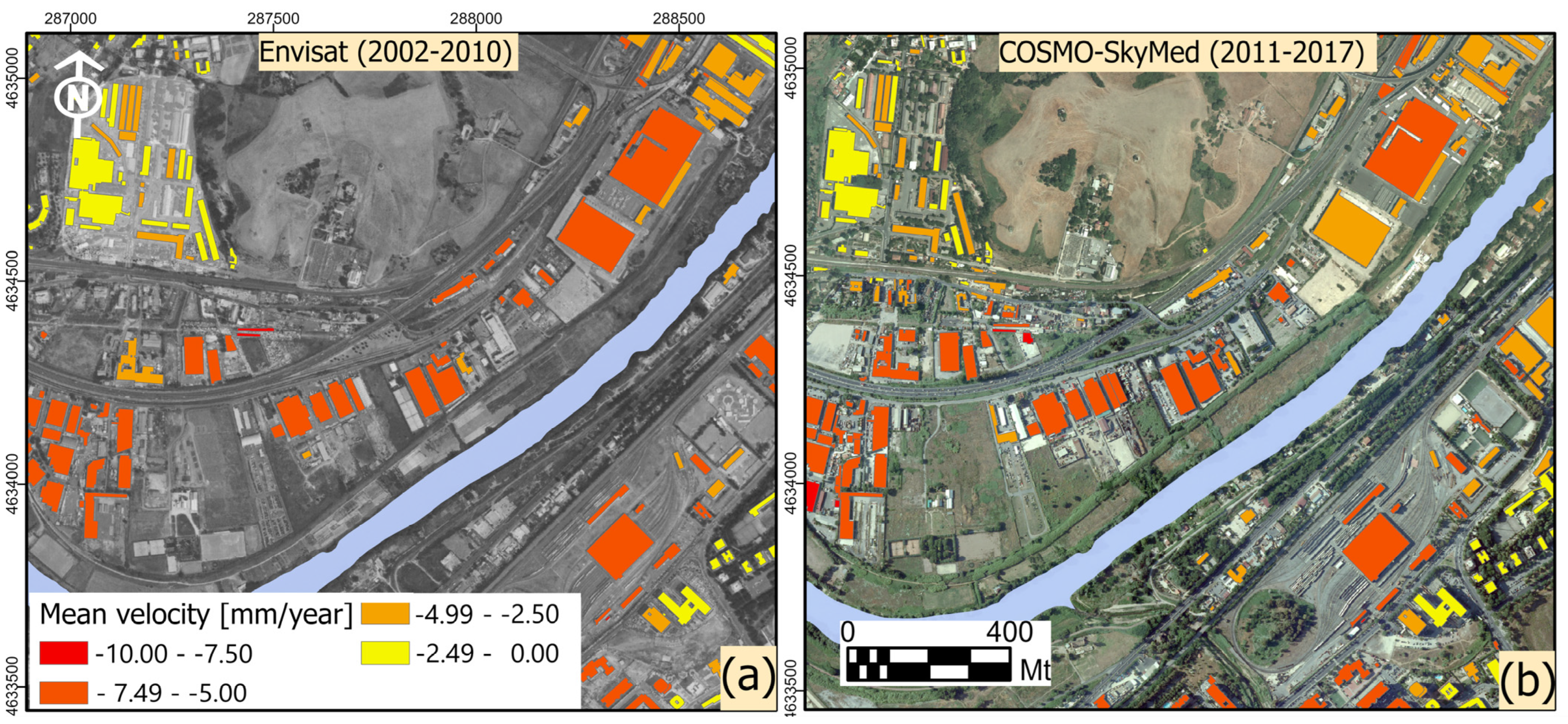
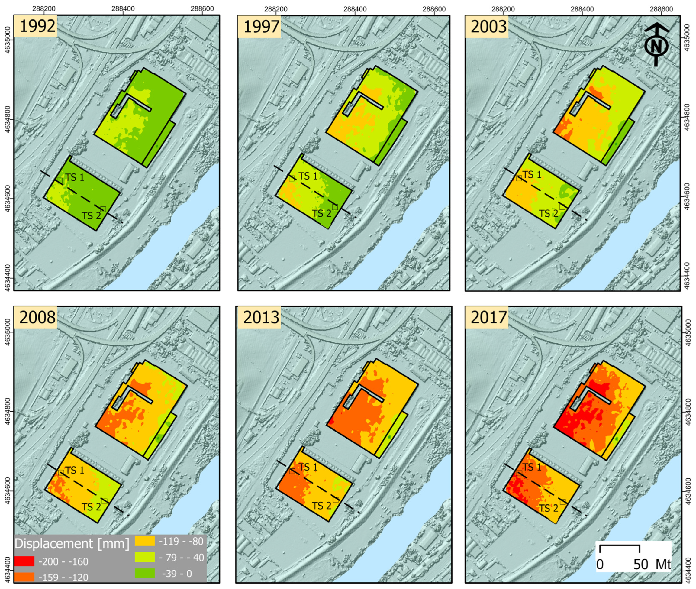
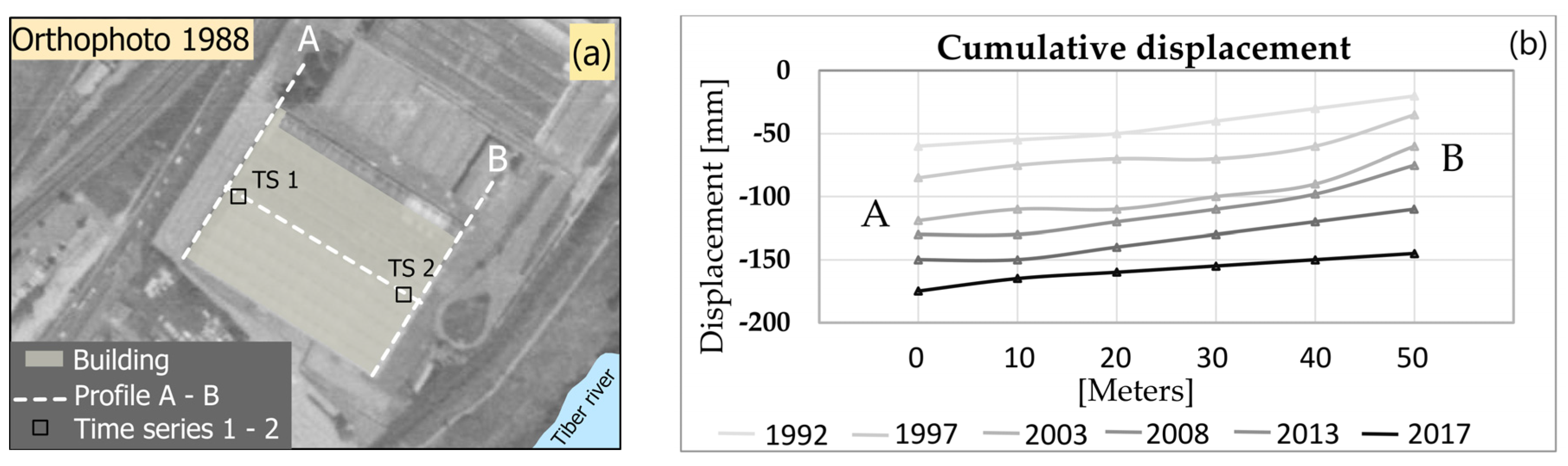
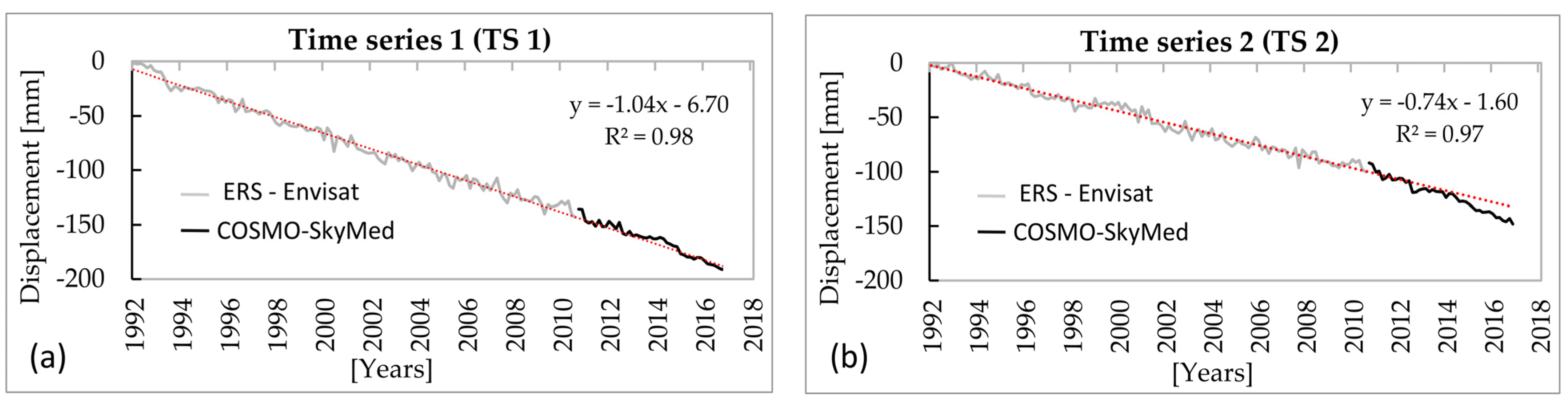
The results are presented and discussed for two area tests: Area 1 (A1) and Area 2 (A2). The measurement point files contain the geographic locations, the coherence value and time series, the vector polygons created by the GIS procedure for each building, and the road sections of the GIS catalog and contain statistical parameters, such as the standard deviation (SD), R2, and mean velocity (mm/year). The interpretation of results and the overlay of measurement points data is done with auxiliary data, such as orthophotos, DSM-LiDAR, and homogenized using the hydrogeological map with the WGS84-UTM 33N Reference System.
The results have found settlement patterns common to other research in the study area, which have been carried out using SAR images from RADARSAT and Sentinel-1 and different PSInSAR, SBAS, IPTA, and 4D SAR processing techniques, e.g., [50,51,52,53,54,55,56]. The main cause of the settlement in this case is the weight of the relatively recent construction on the unconsolidated alluvial material in the southwest periphery of Rome [50]. In addition, there are variations in the water table and groundwater courses that influence the permeability of the soil.
The SAR data from COSMO-SkyMed (2011–2017) have been validated in Orellana et al. [21], using lithological information in the road infrastructures of the Roma-Fiumicino area. In Scifoni et al. [9], the ERS-Envisat data (1992–2010) was validated, using geotechnical models in the Roma Tiber area, confirming the deformations in A1 and A2.

4.1. Area 1

An overall view shows measurement point distribution in Area 1 (A1), including displacement maps from ERS-Envisat (1992–2010) and COSMO-SkyMed (2011–2017), compared with the hydrogeological information of the area and vector cadastral of the DBTR (see Figure 6). The availability of the points is relevant for the measurement of settlements in some structures built before 1992, which allowed the analysis of the evolution of continuous settlements in specific structures, from the first decades of 1992 to 2017 (25 years), which is considered long term for DInSAR observations.
In A1, they have identified anomalies that affect the structures located along the alluvial plain of the Tiber River, where the determining factor is the presence of highly compressible soils (Figure 6a). The displacement velocities V (mm/year) of the measurement points, obtained by ERS-Envisat and COSMO-SkyMed, show displacements homogeneously distributed in large sectors and abnormal velocities, affecting groups of neighboring buildings (see white box in Figure 6c,d). High displacements (red points < −7 mm/year) is observed, within the main valley of the Tiber River, which confirms the supposition that the settlement occurs in geologically homogeneous alluvial areas (black box Figure 6a).
DInSAR has proven to be a valuable geodetic technique for detecting and quantifying the motion of the Earth’s surface (defined as a displacement or rate of velocity). Unlike other geodetic techniques, DInSAR can obtain results from large areas by providing a high spatial resolution of the measurement points. The deformation measurements of the DInSAR are one-dimensional 1D. These measurements are through the Line-Of-Sight (LOS) of the SAR sensor, that is, the line that connects the sensor and the target in question; however, structural motions generally occur in all three spatial dimensions (east (E), north (N), and up (U)). This means that the DInSAR analysis of a stack of synthetic aperture radar (SAR) images acquired in a single viewing geometry is unable to fully capture the magnitude and direction of surface movements.
The spatial density of the DInSAR data has been obtained from the data processing of a satellite orbit, detecting the measurement points. This provides information on ongoing settlement phenomena. It has been observed that a settling trend is generally detected for all satellites and acquisition modes considered ERS, Envisat, and COSMO-SkyMed. Furthermore, it is interesting to note how the use of a single data set (geometric acquisition) can provide meaningful indications for determining the direction of measurement point settlement without using traditional in situ monitoring techniques, such as optical leveling or laser scanning measurements. Figure 7 shows the location, distribution, and comparison of detected measurement points on a structure obtained from two different satellite sensors.
The GIS-based classification procedure through the I.MODI platform allows us to obtain a quick response for structural conditions in urban areas. The procedure is based on the selection of the measurement points detected by the SAR in the structures, where average velocity maps (mm/year) of the point are obtained and calculated for each of the structures present in the land registers or topographic database of Rome (DBTR).
The first test was performed for datasets from ERS-Envisat and COSMO-SkyMed, respectively (see Figure 8). The results show a uniform settlement in the area of the banks of the Tiber River, with a mean velocity of up to −10 (mm/year). Classification combining information on geometric/structural features with deformation measurements can be a friendly tool that can be useful for maintenance and risk management. Through this tool, it will be possible to select sections according to the type of structure and the velocity of movement in order to highlight the critical sections that need careful monitoring in situ. The database of each polygon (vector) allows the selection of data for each individual structure and contains statistical parameters, such as R2, Standard Deviation (SV), and the time series for each of the measurement points.
A detail in structures located on the banks of the Tiber River shows the presence of continuous trends of differential settlement in the temporal coverage of 25 years. Data analysis was carried out in two buildings, where a sufficient number of coherent pixels provided fairly reliable measurement points and cumulative displacement that allowed a long-term settlement period to be reconstructed. The spatial analysis was carried out by quantifying the cumulative displacement, and we proceeded to interpolate with the geostatistical method of ordinary kriging spatial interpolation for the years 1992, 1997, 2003, 2008, 2013, and 2017 (see Figure 9). Trend change in the structure can also be observed by analyzing the cumulative displacement measured using the DInSAR technique (see Figure 10).
Long-term (25-year) trend changes in the structure can be correlated with different settlement patterns, which can give rise to minor local instabilities, as evidenced by the sediment in the settlement area. In some cases, it has been shown that DInSAR monitoring data can also be integrated with traditional monitoring techniques, such as topography, and structural data, for the calculation of differential settlement and numerical modeling in structures, e.g., [9,56].
The time series represents the most advanced DInSAR product. They provide the history of the deformations during the observed period, which is essential for many applications, to study the kinematics of a given phenomenon (inactivity, activation, acceleration, fluctuation, trend changes), and its correlation with inducing factors through the interpretation and exploitation of deformation time series [57,58]. Time series analysis is especially necessary for measurement points with higher consistency; that is, those whose phase terms linked to deformations are more than the model chosen during the processing phase. In fact, it may happen that the measurement point shows significant deformation behavior, due to its high coherence, (usually linear) imposed during the processing phase.
It is important to underline that the time series contain a deformation estimate for each SAR acquisition, that is, for each observation (frame). Therefore, they are especially sensitive to noise [59]. The X-band time series shows a notable improvement in quality with respect to the C-band time series [60]; however, both signals are complementary. The performance of the time series comes from the pixels contained in the SAR image, characterized by a high signal quality; this information is detected in correspondence with the stable reflectors that typically correspond to artificial structures, such as buildings and roads.
The time series ERS-Envisat and COSMO-SkyMed, of two target pixels or points denoted with TS 1 and TS 2 have been selected in the buildings, indicated in Figure 9 and Figure 10a, for the 25-year SAR record continuum. The time series indicates a continuous displacement in the long term, up to 200 mm for TS 1 (see Figure 11a), with an acceleration for TS 2 after 2014 (see Figure 11b). In addition, R2 indicates values close to 1, indicating a good adjustment between the measurements. Therefore, the results of the different satellite sensors are very mutually reliable, indicating a negative displacement trend (differential settlement).

4.2. Area 2

The overall view of Area 2 (A2) shows buildings and highways in a strategic area of Rome (see Figure 12). A2 is characterized as a settlement area in the proximity of the Tiber River, and the groundwater flows are indicated by the blue arrows in the alluvial deposits (Figure 12a). To record the periods of settlement of the structures, a dataset that reaches 15 years of temporal coverage has been used, from the Envisat (2002–2010) and COSMO-SkyMed (2011–2017) satellites, as well as the layers of the Topographic Database of Rome (DBTR), which include road sections and building polygons (see Figure 12b).
Anomalous settlements are observed, within the Tiber River Delta, on the A91 highway and the Roma Fair buildings, with moderate displacement (orange points <−10 mm/year) and high displacement (red points <−15 mm/year). When comparing the SBAS data from Envisat and COSMO-SkyMed, the difference in measurement point density is observed; however, a similarity in velocities (mm/year) is evident (see Figure 12c,d), confirming the consistency of the displacement data for recent structures built after 2006.
Based on the results of the DInSAR velocities, we have found that the embankments of Area 2 are in active movement, identifying some long-term settlement sites along the A91 highway built in 1959 and short-term for car parking built after 2011, both located in the plain and wetlands of the Tiber River Delta. This has made it possible to corroborate the differential settlement in certain types of sediments.
A GIS-based classification test is carried out by associating the measurement points with the DBTR data in A2. An output of the calculated mean velocity was obtained in the 100 mt sections of the A91 Highway, in addition to the buildings in settlements located in the delta of the Tiber River. Both classified datasets reached mean velocities (Vm) of ~ −18 mm/year (see Figure 13a,b). The difference is mainly linked to the large different spatial resolutions of these sensors. Therefore, the same technique applied to different sensors produces different numbers of measurement points. However, the combination of the two datasets allows the reconstruction of a long time series, as already mentioned. The different number of points resulting from using Envisat and COSMO-SkyMed is evident. The difference is mainly related to the great difference in spatial resolution of these sensors; on the A91 motorway with Envisat, there is no data (see Figure 13a). On the contrary, COSMO-SkyMed provides high quality and reliability for structural analysis in infrastructures and buildings (see Figure 13b).
Data integration is achieved by relating the different polygons of the land register that populate the database. The information content in the DBTR is generally a code that uniquely identifies a single record; the common fields are the identification and description of the buildings: Code, Type, Use, Height, Area, etc. By integrating the DInSAR data, new fields are obtained, associated with the stability of the structure, mainly statistical parameters, maximum velocity (Vmax) and minimum velocity (Vmin), mean velocity (Vm), standard deviation (SD), and R2. Table 3 and Table 4 show the new integrated fields for 5 buildings indicated in Figure 13 as A B, C, D, and E.
Envisat (2002–2010) and COSMO-SkyMed (2011–2017) time series indicate that settlement occurred in buildings with shallow foundations and on the embankment of the A91 highway, all interacting with highly compressible alluvial deposits. Through the time series (Figure 14a), linear trend deformation can be seen in TS 3 for 15 years; however, in TS 4 (Figure 14b), from the measurement point of view of the consolidation theory, there is a velocity decrease and a slight tendency toward consolidation of the structure after the year 2014. This result shows interesting perspectives for the potential of SAR interferometry as a tool to predict and calibrate the settlement tendency caused by the construction of new buildings [61] using the velocities and time series obtained by DInSAR.
The results of the roads of A2 show the highest settlement revealed. With Cosmo-SkyMed, we analyzed the potential of the high-resolution analysis that was obtained in DInSAR processing, focusing on the most settled sections of the A91 Highway. The capability of DInSAR to monitor displacements in road infrastructures by observing a large number of points distributed throughout the structure [62] is becoming a powerful and economical means [63,64] for structural health monitoring. To identify the settlement on the A91 highway, a 1.0 km section of road was prepared, where axes 1–2 of sections S-63 and S-61 intersect, respectively. We were able to calculate the mean velocity (mm/year) of all DBTR sections and then classify them in the GIS procedure (see Figure 15a), using between 40 and 60 points per 100 mt section; here, most of the sections detected negative values for mean velocity.
The road sections with the greatest displacement, called S-61 and S-63, are selected. The mean velocity of movement of the S-61 section is −18 mm/year calculated with 57 points, and for S-63, it is −20 mm/year calculated with 61 points. The high density of measurement points is sufficient to reveal detailed settlement conditions in each of the road sections. The A91 highway is designed with 3–4 lanes in both directions of traffic. It is a flat highway with a strategic location, with a high volume of traffic, which can favor settlement and usury. To determine the spatial deformation of the settlement of the road sections, we used the kriging spatial interpolation technique (Figure 15b,c), where we were able to estimate the deformation using the profiles A-A’ of S-61 and B-B’ of S-63, located on axes 1 and 2, respectively.
Using a digital surface model (DSM), with a spatial resolution of 1 mt, derived from LiDAR data from 2011 (see Figure 16a), a topographic profile has been graphed for the year 2017. In axes 1–2 (Figure 16b,c), differential settlement occurs according to the same topographic trend, reaching values of up to 135 [mm] of monitoring with COSMO-SkyMed (2011–2017).

4.3. Settlement Interpretation

The GIS-based application has allowed the identification of structural settlements caused mainly by soil consolidation processes, for different monitoring periods (15–25 years). The classical theories of soil mechanics allow us to consider that, due to these applied external loads. The induced settlement can be considered as the combination of primary consolidation and secondary compression processes (see Figure 17) depending on the conditions of effective stress in situ, of the characteristics of compressibility and related viscosity of the loaded soils, in the thickness of the compressible stratum, and in the time from the moment of loading.
This phenomenon is described and explained by the well-known “Theory of consolidation” of Terzaghi and Peck [65] in terms of dissipation of excess pore pressures induced by external loading in undrained conditions. For both test areas A1 and A2, the primary consolidation time (5–20 years) is exceeded. For the study area, Figure 1 shows that for those mainly composed of alluvial deposits and a fine-grained level, the time needed to complete the primary consolidation process triggered by an external loading depends on the hydraulic conductivity and on drainage conditions and paths, being in some cases (i.e., thick layer of a very low permeability deposits involved in 1D consolidation process) very long, such as some tens of years. The computation method derived from the Terzaghi theory is more complicated when stratified deposits are considered in Lambe and Whitman [66].
The settlement rate in A1 in the Tiber River valley could be explained in terms of the secondary consolidation process. On the other hand, in A2, the main urbanization in the Tiber River delta occurred in more recent times, and the highest rate of settlement could be due to a still active primary consolidation process, strongly dependent on time (Figure 17). Based on this interpretation, a few tens of years seems sufficient time to complete the primary consolidation process due to urbanization; however, for the A91 highway built in 1959 and buildings on the A1, the time required to complete the consolidation process increases primarily to over 50 years due to the existence of lithological peculiarities in alluvial deposits.
The local geological conditions indicate that the load of the infrastructure may be one of the main factors in soil consolidation. However, further analysis is required to characterize settlement-induced phenomena. By using the hydrogeological map of Lazio (see Figure 1), we were able to calculate the mean velocity structure rates for each lithological type interested in by the A1 and A2. In Figure 18, gravel/sands/clay correspond to a low rate of settlement for the mean velocity of measurement points over structures. As expected, unconsolidated deposits, e.g., sands and other alluvial materials, show higher settlement rates compared to basement formations, such as marl and limestone.
Recent alluvial deposits are the most likely to settle as a consequence of the superposition of some external loads, for example, “urbanization”. This term is understood here as the sum of the generic load due to the construction of primary infrastructures, such as roads, railways, aqueducts, and sewers, the construction of buildings, whose load contribution depends on the type of foundation and corresponding depth, artificial fillings to level the surface of the land, and a possible decrease in the water table.
From a hydrogeological standpoint, deformation is interpreted through the well-defined drainage that is present in the Roma-Fiumicino area, where the alluvial valleys show prominent and steep banks that border the alluvial plains on the Roma-Fiumicino highway and its surroundings. This network originated during the Pleistocene when the fall of the sea level produced repeated downward cuts of the riverbeds [50]. It can be pointed out that the mechanisms of soil consolidation are potentially increased by the type of soil, mainly in areas prone to deformation. However, in the case of local deformations in infrastructures, these can be caused by specific structural failures, determined, for example, by the type of foundation or external usury loads on the structures.

5. Conclusions

The paper illustrates a service that was tested on datasets using Envisat data (a mission that ended in 2012) and COSMO-SkyMed that it is still operative and available on-demand all over the world with minor limitations, eventually posed by interference with non-civil operations. In the future, Sentinel 1 datasets and other active SAR missions can be used to collect data to be processed. The GIS application does not depend on a specific satellite mission since it is based on the availability of large data set for the generation of time series.
DInSAR differential interferometry provided a comprehensive analysis of surface displacements in test areas A1 and A2. Using back and recent satellite data is invaluable for analyzing travel patterns at different scales and for specific infrastructure components, such as highway structures and buildings. The first SAR images available since 1992 are very relevant for studying and reconstructing periods of historical deformation. The most recent high-resolution satellite data, such as SAR images from COSMO-SkyMed, are relevant for determining spatial deformation due to their density of measurement points. Post-processing and GIS analysis allowed us to know the behavior in great detail.
In particular, most of the specific target points detected in infrastructures allowed us to understand the temporal behavior during the investigated period. Through the measurement point maps, annual velocities indices, cumulated displacements, mean velocities, and profile estimation, it showed us the DInSAR potential to detect the settlement that affects the roads and buildings that are located in the alluvial lands of the Tiber River hydrographic network.
GIS-based classification has identified relatively more stable structures within A1 and A2. We infer that the observed settlement is time dependent, even on a long time scale, with respect to the age of the infrastructure. In fact, the classification of the mean velocities (Vm), together with the R2 and SD parameters, showed that most of the infrastructure structures that cross the area show continuous settlement, which affects all alluvial deposits after urbanization. The velocity maps showed that a general settlement affects the buildings that sit on alluvial deposits. In addition, two distinct trends are recognized within this geologically homogeneous sector: a moderate settlement (<−5 mm/year) within the main valley of the Tiber River and a high settlement (<−10 mm/year) in the Tiber River Delta.
The results of structural settlements revealed that the highest settlement values were observed in the western part of the Tiber delta, on the A91 road, and, to a lesser extent, in the center of Rome. These structures are located in a geologically complex area due to the dynamics of the Tiber delta, which is affected by unconsolidated soils and underground water courses. The greatest displacements are close to the Tiber River and are probably due to the presence of consolidation phenomena still underway, boosted by external loads from storage in logistics and commercial buildings. The analyses carried out do not replace the direct survey but allow us to build an overview of the settlement in the structures of the study area and could be used as a reference for maintenance and safety programs aimed at mitigating the potential risk. The results also highlight the importance of applying the DInSAR technique in the long term; the longer time window allows a more precise analysis of slow settlements, and the use of multiple constellations allows validation of spatiotemporal trends in displacements between the different satellite sensors.

Author Contributions

Conceptualization, F.O., P.J.V.D., S.S. and M.M.; methodology, F.O., P.J.V.D., S.S. and M.M.; software, F.O. and P.J.V.D.; validation, F.O. and P.J.V.D.; writing F.O.; supervision, P.J.V.D. and M.M. All authors have read and agreed to the published version of the manuscript.

Funding

This research received no external funding.

Institutional Review Board Statement

Not applicable.

Informed Consent Statement

Not applicable.

Data Availability Statement

The Hydrogeological map of Rome is available from La Vigna et al. [43], under license: https://creativecommons.org/licenses/by-nc/4.0/. The Envisat, LiDAR data, and orthophotos is available on the Italian National Geoportal http://www.pcn.minambiente.it/mattm/ (accessed on 16 August 2022), under the INSPIRE license http://www.pcn.minambiente.it/mattm/en/inspire/ The long time series was carried out with ERS-Envisat dataset and was processed by Scifoni et al. [9], under a collaboration with CNR-IREA-Italian National Research Council and the spin-off Survey Lab-Sapienza. The Envisat dataset was provided by the Ministry of the Environment and the Protection of the Territory and the Sea, through the Italian national geoportal.

Acknowledgments

We acknowledge the I.MODI Project, funded by Horizon 2020—SME, I.MODI proposal, development and instrument phase 2, Grant agreement No 720121. For COSMO- SkyMed data, the project was carried out using the COSMO-SkyMed ® Product © ASI (Italian Space Agency) provided under license by ASI. The authors also wish to thank the contributions of Manuela Bonano and Riccardo Lanari from IREA—CNR Italy, for providing valuable information on the quality of the DInSAR data, within the scope of a scientific collaboration for the I.MODI project.

Conflicts of Interest

The authors declare no conflict of interest.

References

  1. Gigli, G.; Fanti, R.; Canuti, P.; Casagli, N. Integration of advanced monitoring and numerical modeling techniques for the complete risk scenario analysis of rockslides: The case of Mt. Beni (Florence, Italy). Eng. Geol. 2011, 120, 48–59. [Google Scholar] [CrossRef]
  2. Bru, G.; González, P.J.; Mateos, R.M.; Roldán, F.J.; Herrera, G.; Béjar-Pizarro, M.; Fernández, J. A-dinsar monitoring of landslide and subsidence activity: A case of urban damage in Arcos de la Frontera, Spain. Remote Sens. 2017, 9, 787. [Google Scholar] [CrossRef]
  3. D’Amico, F.; Gagliardi, V.; Bianchini Ciampoli, L.; Tosti, F. Integration of InSAR and GPR techniques for monitoring transition areas in railway bridges. NDT E Int. 2020, 115, 102291. [Google Scholar] [CrossRef]
  4. Bianchini Ciampoli, L.; Gagliardi, V.; Clementini, C.; Latini, D.; Del Frate, F.; Benedetto, A. Transport infrastructure monitoring by InSAR and GPR data fusion. Surv. Geophys. 2020, 41, 371–394. [Google Scholar] [CrossRef]
  5. Beshr, A.A.; Abo Elnaga, I.M. Investigating the accuracy of digital levels and reflectorless total stations for purposes of geodetic engineering. Alex. Eng. J. 2011, 50, 399–405. [Google Scholar] [CrossRef]
  6. Lienhart, W. Geotechnical monitoring using total stations and laser scanners: Critical aspects and solutions. J. Civ. Struct. Health Monit. 2017, 7, 315–324. [Google Scholar] [CrossRef]
  7. Miano, A.; Di Carlo, F.; Mele, A.; Giannetti, I.; Nappo, N.; Rompato, M.; Striano, P.; Bonano, M.; Bozzano, F.; Lanari, R.; et al. GIS Integration of DInSAR Measurements, Geological Investigation and Historical Surveys for the Structural Monitoring of Buildings and Infrastructures: An Application to the Valco San Paolo Urban Area of Rome. Infrastructures 2022, 7, 89. [Google Scholar] [CrossRef]
  8. Bianchini, S.; Ciampalini, A.; Raspini, F.; Bardi, F.; Di Traglia, F.; Moretti, S.; Casagli, N. Multi-temporal evaluation of landslide movements and impacts on buildings in San Fratello (Italy) by means of C-band and X-band PSI data. Pure Appl. Geophys. 2015, 172, 3043–3065. [Google Scholar] [CrossRef]
  9. Scifoni, S.; Bonano, M.; Marsella, M.; Sonnessa, A.; Tagliafierro, V.; Manunta, M.; Lanari, R.; Ojha, C.; Sciotti, M. On the joint exploitation of long-term DInSAR time series and geological information for the investigation of ground settlements in the town of Roma (Italy). Remote Sens. Environ. 2016, 182, 113–127. [Google Scholar] [CrossRef]
  10. Arangio, S.; Calò, F.; Di Mauro, M.; Bonano, M.; Marsella, M.; Manunta, M. An application of the SBAS-DInSAR technique for the assessment of structural damage in the city of Rome. Struct. Infrastruct. Eng. 2014, 10, 1469–1483P. [Google Scholar] [CrossRef]
  11. Peduto, D.; Ferlisi, S.; Nicodemo, G.; Reale, D.; Pisciotta, G.; Gullà, G. Empirical fragility and vulnerability curves for buildings exposed to slow-moving landslides at medium and large scales. Landslides 2017, 14, 1993–2007. [Google Scholar] [CrossRef]
  12. Sousa, J.J.; Bastos, L.F.S. Multi-temporal SAR interferometry reveals acceleration of bridge sinking before collapse. Nat. Hazards Earth Syst. Sci. 2013, 13, 659–667. [Google Scholar] [CrossRef]
  13. Lazecky, M.; Hlaváčová, I.; Bakon, M.; Sousa, J.J.; Perissin, D.; Patricio, G. Bridge Displacements Monitoring Using Space-Borne X-Band SAR Interferometry. IEEE J. Sel. Top. Appl. Earth Obs. Remote Sens. 2016, 10, 205–210. [Google Scholar] [CrossRef]
  14. Chang, L.; Dollevoet, R.P.B.J.; Hanssen, R.F. Nationwide Railway Monitoring Using Satellite SAR Interferometry. IEEE J. Sel. Top. Appl. Earth Obs. Remote Sens. 2016, 10, 596–604. [Google Scholar] [CrossRef]
  15. Luo, Q.; Zhou, G.; Perissin, D. Monitoring of Subsidence along Jingjin Inter-City Railway with High-Resolution TerraSAR-X MT-InSAR Analysis. Remote Sens. 2017, 9, 717. [Google Scholar] [CrossRef]
  16. Perissin, D.; Wang, Z.; Lin, H. Shanghai subway tunnels and highways monitoring through Cosmo-SkyMed Persistent Scatterers. ISPRS J. Photogramm. Remote Sens. 2012, 73, 58–67. [Google Scholar] [CrossRef]
  17. Martí, J.G.; Nevard, S.; Sanchez, J. The Use of InSAR (Interferometric Synthetic Aperture Radar) to Complement Control of Construction and Protect Third Party Assets; Crossrail Learning Legacy Report; Crossrail Ltd.: London, UK, 2017. [Google Scholar]
  18. Milillo, P.; Giardina, G.; DeJong, M.J.; Perissin, D.; Milillo, G. Multi-Temporal InSAR Structural Damage Assessment: The London Crossrail Case Study. Remote Sens. 2018, 10, 287. [Google Scholar] [CrossRef]
  19. Vaccari, A.; Batabyal, T.; Tabassum, N.; Hoppe, E.; Bruckno, B.S.; Acton, S.T. Integrating Remote Sensing Data in Decision Support Systems for Transportation Asset Management. Transp. Res. Rec. J. Transp. Res. Board 2018, 2672, 23–35. [Google Scholar] [CrossRef]
  20. Infante, D.; Di Martire, D.; Confuorto, P.; Tessitore, S.; Ramondini, M.; Calcaterra, D. Differential Sar Interferometry Technique for Control of Linear Infrastructures Affected by Ground Instability Phenomena. ISPRS Int. Arch. Photogramm. Remote Sens. Spat. Inf. Sci. 2018, 3, 251–258. [Google Scholar] [CrossRef]
  21. Orellana, F.; Delgado Blasco, J.M.; Foumelis, M.; D’Aranno, P.J.; Marsella, M.A.; Di Mascio, P. Dinsar for road infrastructure monitoring: Case study highway network of Rome metropolitan (Italy). Remote Sens. 2020, 12, 3697. [Google Scholar] [CrossRef]
  22. Grassi, F.; Mancini, F.; Bassoli, E.; Vincenzi, L. Contribution of anthropogenic consolidation processes to subsidence phenomena from multi-temporal DInSAR: A GIS-based approach. GIScience Remote Sens. 2022, 59, 1901–1917. [Google Scholar] [CrossRef]
  23. Aditiya, A.; Aoki, Y.; Anugrah, R.D. Surface deformation monitoring of Sinabung volcano using multi temporal InSAR method and GIS analysis for affected area assessment. In IOP Conference Series: Materials Science and Engineering, Proceedings of the 3rd International Conference on Science, Technology, and Interdisciplinary Research (IC-STAR), Bandar Lampung City, Indonesia, 18–20 September 2017; IOP Publishing: Bristol, UK, 2018; Volume 344, No. 1; p. 012003. [Google Scholar] [CrossRef]
  24. Devara, M.; Tiwari, A.; Dwivedi, R. Landslide susceptibility mapping using MT-InSAR and AHP enabled GIS-based multi-criteria decision analysis. Geomat. Nat. Hazards Risk 2021, 12, 675–693. [Google Scholar] [CrossRef]
  25. Liu, Z.; Mei, G.; Sun, Y.; Xu, N. Investigating mining-induced surface subsidence and potential damages based on SBAS-InSAR monitoring and GIS techniques: A case study. Environ. Earth Sci. 2021, 80, 817. [Google Scholar] [CrossRef]
  26. Ferretti, A.; Prati, C.; Rocca, F. Permanent scatterers in SAR interferometry. IEEE Trans. Geosci. Remote Sens. 2001, 39, 8–20. [Google Scholar] [CrossRef]
  27. Berardino, P.; Fornaro, G.; Lanari, R.; Sansosti, E. A new algorithm for surface deformation monitoring based on small baseline 641 differential SAR interferograms. IEEE Trans. Geosci. Remote Sens. 2002, 40, 2375–2383. [Google Scholar] [CrossRef]
  28. Werner, C.; Wegmuller, U.; Strozzi, T.; Wiesmann, A. Interferometric point target analysis for deformation mapping. In Proceedings of the IGARSS 2003, IEEE International Geoscience and Remote Sensing Symposium (IEEE Cat. No. 03CH37477), Toulouse, France, 21–25 July 2003; IEEE: New York, NY, USA, 2004; Volume 7, pp. 4362–4364. [Google Scholar] [CrossRef]
  29. Lanari, R.; Mora, O.; Manunta, M.; Mallorquí, J.J.; Berardino, P.; Sansosti, E. A small-baseline approach for investigating deformations on full-resolution differential SAR interferograms. IEEE Trans. Geosci. Remote Sens. 2004, 42, 1377–1386. [Google Scholar] [CrossRef]
  30. Ferretti, A.; Fumagalli, A.; Novali, F.; Prati, C.; Rocca, F.; Rucci, A. A new algorithm for processing interferometric data-stacks: SqueeSAR. IEEE Trans. Geosci. Remote Sens. 2011, 49, 3460–3470. [Google Scholar] [CrossRef]
  31. Casu, F.; Manzo, M.; Lanari, R. A quantitative assessment of the SBAS algorithm performance for surface deformation retrieval from DInSAR data. Remote Sens. Environ. 2006, 102, 195–210. [Google Scholar] [CrossRef]
  32. Lanari, R.; Casu, F.; Manzo, M.; Lundgren, P. Application of the SBAS-DInSAR technique to fault creep: A case study of the Hayward fault, California. Remote Sens. Environ. 2007, 109, 20–28. [Google Scholar] [CrossRef]
  33. Bonano, M.; Manunta, M.; Pepe, A.; Paglia, L.; Lanari, R. From previous C-band to new X-band SAR systems: Assessment of the DInSAR mapping improvement for deformation time-series retrieval in urban areas. IEEE Trans. Geosci. Remote Sens. 2013, 51, 1973–1984. [Google Scholar] [CrossRef]
  34. Orellana, F.; Hormazábal, J.; Montalva, G.; Moreno, M. Measuring Coastal Subsidence after Recent Earthquakes in Chile Central Using SAR Interferometry and GNSS Data. Remote Sens. 2022, 14, 1611. [Google Scholar] [CrossRef]
  35. Orellana, F.; Moreno, M.; Yáñez, G. High-Resolution Deformation Monitoring from DInSAR: Implications for Geohazards and Ground Stability in the Metropolitan Area of Santiago, Chile. Remote Sens. 2022, 14, 6115. [Google Scholar] [CrossRef]
  36. Chang, L.; Dollevoet, R.P.; Hanssen, R.F. Monitoring line-infrastructure with multisensor SAR interferometry: Products and performance assessment metrics. IEEE J. Sel. Top. Appl. Earth Obs. Remote Sens. 2018, 11, 1593–1605. [Google Scholar] [CrossRef]
  37. Di Martire, D.; Paci, M.; Confuorto, P.; Costabile, S.; Guastaferro, F.; Verta, A.; Calcaterra, D. A nation-wide system for landslide mapping and risk management in Italy: The second Not-ordinary Plan of Environmental Remote Sensing. Int. J. Appl. Earth Obs. Geoinf. 2017, 63, 143–157. [Google Scholar] [CrossRef]
  38. Crosetto, M.; Solari, L.; Mróz, M.; Balasis-Levinsen, J.; Casagli, N.; Frei, M.; Oyen, A.; Moldestad, D.A.; Bateson, L.; Guerrieri, L.; et al. The evolution of wide-area DInSAR: From regional and national services to the European Ground Motion Service. Remote Sens. 2020, 12, 2043. [Google Scholar] [CrossRef]
  39. Milillo, P.; Giardina, G.; Perissin, D.; Milillo, G.; Coletta, A.; Terranova, C. Pre-Collapse Space Geodetic Observations of Critical Infrastructure: The Morandi Bridge, Genoa, Italy. Remote Sens. 2019, 11, 1403. [Google Scholar] [CrossRef]
  40. De Luca, C.; Bonano, M.; Casu, F.; Fusco, A.; Lanari, R.; Manunta, M.; Manzo, M.; Pepe, A.; Zinno, I. Automatic and systematic Sentinel-1 SBAS-DInSAR processing chain for deformation time-series generation. Procedia Comput. Sci. 2016, 100, 1176–1180. [Google Scholar] [CrossRef]
  41. Milli, S.; D’Ambrogi, C.; Bellotti, P.; Calderoni, G.; Carboni, M.G.; Celant, A.; Di Bella, L.; Di Rita, F.; Frezza, V.; Magri, D.; et al. The transition from wave-dominated estuary to wave-dominated delta: The Late Quaternary stratigraphic architecture of Tiber River deltaic succession (Italy). Sediment. Geol. 2013, 284, 159–180. [Google Scholar] [CrossRef]
  42. Mancini, M.; Moscatelli, M.; Stigliano, F.; Cavinato, G.P.; Marini, M.; Milli, S.; Simionato, M.; Cosentino, G.; Polpetta, F. Middle Pleistocene fluvial incised valleys from the subsoil of the centre of Rome: Facies, stacking pattern and controls on sedimentation. In Proceedings of the Congresso Nazionale della Società Geologica Italiana–Geosciences on a Changing Planet: Learning from the Past, Exploring the Future, Napoli, Italy, 7–9 September 2016. [Google Scholar]
  43. La Vigna, F.; Mazza, R.; Amanti, M.; Di Salvo, C.; Petitta, M.; Pizzino, L. The synthesis of decades of groundwater knowledge: The new Hydrogeological Map of Rome. Acque Sotter. Ital. J. Groundw. 2015, 4. [Google Scholar] [CrossRef]
  44. La Vigna, F.; Mazza, R.; Amanti, M.; Di Salvo, C.; Petitta, M.; Pizzino, L.; Pietrosante, A.; Martarelli, L.; Bonfà, I.; Capelli, G.; et al. Groundwater of Rome. J. Maps 2016, 12 (Suppl. 1), 88–93. [Google Scholar] [CrossRef]
  45. Mazza, R.; La Vigna, F.; Capelli, G.; Dimasi, M.; Mancini, M.; Mastrorillo, L. Idrogeologia del territorio di Roma. Acque Sotter. It. J. Groundw 2016, 4, 19–30. [Google Scholar]
  46. Bozzano, F.; Esposito, C.; Mazzanti, P.; Patti, M.; Scancella, S. Imaging Multi-Age Construction Settlement Behavior by Advanced SAR Interferometry. Remote Sens. 2018, 10, 1137. [Google Scholar] [CrossRef]
  47. Cappelli, G.; Mazza, R.; Taviani, S. Acque sotterranee nella città di Roma. Mem. Descr. Carta Geol. D’it. 2008, 80, 221–245. [Google Scholar]
  48. Di Salvo, C.; Di Luzio, E.; Mancini, M.; Moscatelli, M.; Capelli, G.; Cavinato, G.P.; Mazza, R. GIS-based hydrostratigraphic modeling of the city of Rome (Italy): Analysis of the geometric relationships between a buried aquifer in the Tiber Valley and the confining hydrostratigraphic complexes. Hydrogeol. J. 2012, 20, 1549. [Google Scholar] [CrossRef]
  49. Zebker, H.A.; Villasenor, J. Decorrelation in interferometric radar echoes. IEEE Trans. Geosci. Remote Sens. 1992, 30, 950–959. [Google Scholar] [CrossRef]
  50. Stramondo, S.; Bozzano, F.; Marra, F.; Wegmuller, U.; Cinti, F.R.; Moro, M.; Saroli, M. Subsidence induced by urbanisation in the city of Rome detected by advanced InSAR technique and geotechnical investigations. Remote Sens. Environ. 2008, 112, 3160–3172. [Google Scholar] [CrossRef]
  51. Manunta, M.; Marsella, M.; Zeni, G.; Sciotti, M.; Atzori, S.; Lanari, R. Two-scale surface deformation analysis using the SBAS-DInSAR technique: A case study of the city of Rome, Italy. Int. J. Remote Sens. 2008, 29, 1665–1684. [Google Scholar] [CrossRef]
  52. Fornaro, G.; Serafino, F.; Reale, D. 4-D SAR imaging: The case study of Rome. IEEE Geosci. Remote Sens. Lett. 2010, 7, 236–240. [Google Scholar] [CrossRef]
  53. Comerci, V.; Cipolloni, C.; di Manna, P.; Guerrieri, L.; Vittori, E.; Bertoletti, E.; Ciuffreda, M.; Succhiarelli, C. PanGeo: Enabling Access to Geological Information in Support of GMES-D7.1.26 Geohazard Description for Rome. 2012. Available online: https://nora.nerc.ac.uk/id/eprint/19289 (accessed on 23 May 2022).
  54. Cigna, F.; Lasaponara, R.; Masini, N.; Milillo, P.; Tapete, D. Persistent scatterer interferometry processing of COSMO-skymed stripmap HIMAGE time series to depict deformation of the historic centre of Rome, Italy. Remote Sens. 2014, 6, 12593–12618. [Google Scholar] [CrossRef]
  55. Delgado Blasco, J.M.D.; Foumelis, M.; Stewart, C.; Hooper, A. Measuring Urban Subsidence in the Rome Metropolitan Area (Italy) with Sentinel-1 SNAP-StaMPS Persistent Scatterer Interferometry. Remote Sens. 2019, 11, 129. [Google Scholar] [CrossRef]
  56. D’Aranno, P.J.; Marsella, M.; Scifoni, S.; Scutti, M.; Sonnessa, A.; Bonano, M. Advanced DInSAR analysis for building damage assessment in large urban areas: An application to the city of Roma, Italy. In Proceedings of the SPIE 9642, SAR Image Analysis, Modeling, and Techniques XV, Toulouse, France, 23 October 2015; p. 96420L. [Google Scholar] [CrossRef]
  57. Crosetto, M.; Monserrat, O.; Cuevas-González, M.; Devanthéry, N.; Crippa, B. Persistent scatterer interferometry: A review. ISPRS J. Photogramm. Remote Sens. 2016, 115, 78–89. [Google Scholar] [CrossRef]
  58. Orellana, F.; Rivera, D.; Montalva, G.; Arumi, J.L. InSAR-Based Early Warning Monitoring Framework to Assess Aquifer Deterioration. Remote Sens. 2023, 15, 1786. [Google Scholar] [CrossRef]
  59. Crosetto, M.; Monserrat, O.; Adam, N.; Parizzi, A.; Bremmer, C.; Dortland, S.; van Leijen, F.J. Final report of the Validation of existing processing chains in Terrafirma stage 2. Terrafirma project, ESRIN. Contract 2008, 19366. [Google Scholar] [CrossRef]
  60. Crosetto, M.; Monserrat, O.; Iglesias, R.; Crippa, B. Persistent scatterer interferometry: Potential, limits and initial C-and X-band comparison. Photogramm. Eng. Remote Sens. 2010, 76, 1061–1069. [Google Scholar] [CrossRef]
  61. Moretto, S.; Bozzano, F.; Esposito, C.; Mazzanti, P.; Rocca, A. bAssessment of landslide pre-failure monitoring and forecasting using satellite SAR interferometry. Geosciences 2017, 7, 36. [Google Scholar] [CrossRef]
  62. D’Aranno, P.; Di Benedetto, A.; Fiani, M.; Marsella, M. Remote sensing technologies for linear infrastructure monitoring. Int. Arch. Photogramm. Remote Sens. Spat. Inf. Sci. 2019, 42, 461–468. [Google Scholar] [CrossRef]
  63. Milillo, P.; Riel, B.; Minchew, B.; Yun, S.-H.; Simons, M.; Lundgren, P. On the Synergistic Use of SAR Constellations Data Exploitation for Earth Science and Natural Hazard Response. IEEE J. Sel. Top. Appl. Earth Obs. Remote Sens. 2016, 9, 1095–1100. [Google Scholar] [CrossRef]
  64. Chen, F.; Wu, Y.; Zhang, Y.; Parcharidis, I.; Ma, P.; Xiao, R.; Xu, J.; Zhou, W.; Tang, P.; Foumelis, M. Surface Motion and Structural Instability Monitoring of Ming Dynasty City Walls by Two-Step Tomo-PSInSAR Approach in Nanjing City, China. Remote Sens. 2017, 9, 371. [Google Scholar] [CrossRef]
  65. Terzaghi, K.; Peck, R.B.; Mesri, G. Soil Mechanics in Engineering Practice; John Wiley & Sons: Hoboken, NJ, USA, 1967. [Google Scholar]
  66. Lambe, T.W.; Whitman, R.V. Soil Mechanics; John Wiley & Sons: Hoboken, NJ, USA, 1979; Volume 10. [Google Scholar]
Figure 1. Hydrogeological map of Rome Tiber delta in black box, Area 1 (A1) and Area 2 (A2) in red boxes (modified from La Vigna et al. [43]).
Infrastructures 08 00094 g001
Figure 2. Infrastructure and urbanization reconstruction from orthophotos 1988, 2000, 2006, and 2012, Area 1 (A1) and Area 2 (A2) in white boxes.
Infrastructures 08 00094 g002
Figure 3. Topographic Data Base of Rome (DBTR) contains land registers (buildings and roads).
Infrastructures 08 00094 g003
Figure 4. SAR data set in study area, background Sentinel 2 image 2022.
Infrastructures 08 00094 g004
Figure 5. GIS ingestion workflow in the I.MODI platform.
Infrastructures 08 00094 g005
Figure 6. Overall View, (a) Location Area 1 (A1) in Hydrogeological map of Rome, (b) Topographic database of Rome (DBTR) including land registers of buildings and roads for A1, (c) Displacement map from ERS-Envisat (1992–2010), and (d) Displacement map from COSMO-SkyMed (2011–2017).
Infrastructures 08 00094 g006
Figure 7. Measurement point distribution over structures, (a) ERS-Envisat (1992–2010) in orthophoto 1988, and (b) COSMO-SkyMed (2011–2017) in orthophoto 2012.
Infrastructures 08 00094 g007
Figure 8. Structure map classification in A1, according to mean velocity (Vm), (a) ERS-Envisat (1992–2010) in orthophoto 1988, and (b) COSMO-SkyMed (2011–2017) in orthophoto 2012.
Infrastructures 08 00094 g008
Figure 9. Detailed displacement temporal evolution for years 1992, 1997, 2003, 2008, 2013, and 2017, Time series in TS 1 and TS 2; deformation cross section in black line; overlay Digital Surface Model (DSM) from LiDAR.
Infrastructures 08 00094 g009
Figure 10. (a) Deformation profile A—B, TS 1, and TS 2 location; (b) Cumulative displacement trend for the years 1992, 1997, 2003, 2013, and 2017.
Infrastructures 08 00094 g010
Figure 11. Time series for 25-year observations from Envisat (2002–2010) and COSMO-SkyMed (2011–2017), (a) Time series 1 (TS 1), and (b) Time series 2 (TS 2).
Infrastructures 08 00094 g011
Figure 12. Overall view: (a) Location Area 2 (A2) in Hydrogeological map of Rome, (b) Topographic database of Rome (DBTR) includes land registers of buildings and roads, (c) Displacement map from ERS-Envisat (2002–2010), and (d) Displacement map from COSMO-SkyMed (2011–2017).
Infrastructures 08 00094 g012
Figure 13. Structures maps classification in Area 2 (A2) according to mean velocity (Vm), (a) Envisat (2002–2010) in orthophoto 2006, and (b) COSMO-SkyMed (2011–2017) in orthophoto 2012. TS 3 and TS 4 indicated time series.
Infrastructures 08 00094 g013
Figure 14. Time series for 15-year observations from Envisat (2002–2010) and COSMO-SkyMed (2011–2017), (a) Time series 3 (TS 3), and (b) Time series 4 (TS 4), shown in Figure 13.
Infrastructures 08 00094 g014
Figure 15. (a) Road section classification in Area 2 (A2), according to mean velocity (Vm), (b) Spatial deformation for section S-61, and (c) Spatial deformation for section S-63 in orthophoto 2012.
Infrastructures 08 00094 g015
Figure 16. (a) Topographic profile carriageway A91 extracted Digital Surface Model (DSM) in 1 mt resolution, (b) Cumulative displacement A-A’ in axis 1, and (c) Cumulative displacement B-B’ in axis 2, using COSMO-SkyMed (2011–2017).
Infrastructures 08 00094 g016
Figure 17. Theory about settlement induced by urbanization. In the upper part: load vs. time; in the lower part: settlement vs. time. SCU: settlement contemporaneous to urbanization; SPC: settlement induced by the primary consolidation process; SSC: settlement induced by the secondary consolidation process (modified from Stramondo et al. [50]).
Infrastructures 08 00094 g017
Figure 18. Settlement by lithological type, calculated from the mean velocity [mm/year] recorded in the structures.
Infrastructures 08 00094 g018
Table 1. Data collection.
Data Year
Orthophoto1988
Orthophoto2000
Orthophoto2006
LiDAR and Digital Surface Model (DSM)2011
Orthophoto2012
Buildings Layers SHP format from DBTR2014
Roads Layers SHP from DBTR2014
Rome Hydrogeological map (scale: 1: 50,000)2015
Table 2. SAR data set.
Data Temporal Cover SAR Band/Wavelength OrbitN° Images
ERS-Envisat 1992–2010C/5.6 cmDescending137
Envisat2002–2010C/5.6 cmDescending59
COSMO-SkyMed2011–2017X/3.1 cmDescending67
Table 3. Building stability indicator from Envisat (2002–2010).
Building N° Measurement Points Vm (mm/Year) SDR2
A15−12.30.830.73
B18−14.50.410.69
C22−18.20.230.89
D26−10.50.370.81
E29−16.20.560.75
Table 4. Building stability indicator from COSMO-SkyMed (2011–2017).
Building N° Measurement Points Vm (mm/Year) SDR2
A28−11.40.890.95
B37−12.10.520.88
C29−12.80.440.72
D43−8.50.530.83
E47−11.90.750.91
Disclaimer/Publisher’s Note: The statements, opinions and data contained in all publications are solely those of the individual author(s) and contributor(s) and not of MDPI and/or the editor(s). MDPI and/or the editor(s) disclaim responsibility for any injury to people or property resulting from any ideas, methods, instructions or products referred to in the content.

