Article

Image-Based Corrosion Detection in Ancillary Structures

Department of Civil Engineering, College of Engineering & Mine, University of North Dakota, 243 Centenial Drive Stop 8115, Grand Forks, ND 58202-8115, USA
*
Author to whom correspondence should be addressed.
Infrastructures 2023, 8(4), 66; https://doi.org/10.3390/infrastructures8040066
Submission received: 10 February 2023 / Revised: 17 March 2023 / Accepted: 27 March 2023 / Published: 28 March 2023

Abstract

:
Ancillary structures are essential for highways’ safe operationality but are mainly prone to environmental corrosion. The traditional way of inspecting ancillary structures is manned inspection, which is laborious, time-consuming, and unsafe for inspectors. In this paper, a novel image processing technique was developed for autonomous corrosion detection of in-service ancillary structures. The authors successfully leveraged corrosion features in the YCbCr color space as an alternative to the conventional red–green–blue (RGB) color space. The proposed method included a preprocessing operation including contrast adjustment, histogram equalization, adaptive histogram equalization, and optimum value determination of brightness. The effect of preprocessing was evaluated against a semantically segmented ground truth as a set of pixel-level annotated images. The false detection rate was higher in Otsu than in the global threshold method; therefore, the preprocessed images were converted to binary using the global threshold value. Finally, an average accuracy and true positive rate of 90% and 70%, respectively, were achieved for corrosion prediction in the YCbCr color space.

1. Introduction

Most ancillary structures, such as high-mast light towers, cantilevered sign structures, overhead traffic signals, and luminaires, are continuously exposed to wind-related fatigue cracks, vibration issues, missing bolts, and loosened nuts [1]. However, corrosion can be considered as the most common defect in them. In ancillary structures, corrosion is caused by factors such as exposure to weather elements, chemicals, and salt compounds. Traditional inspection methods, such as visual and physical nondestructive evaluations (NDEs), can be time-consuming, expensive, complex, dangerous, and even impossible for inaccessible areas. The outcome of the manned evaluations is typically subjective and inconsistent. It is possible that accuracy depends on the inspector’s experience and location’s accessibility for inspection [2]; however, visual inspections remain the most common method for corrosion damage assessment. Maintenance and protection of traffic (MPT) safety legislation demands make it further challenging for stakeholders to perform in-service ancillary structure physical and visual inspections [3]. Therefore, developing noncontact methods augmented with artificial intelligence (AI) as an alternative to conventional defect detection is a necessity.
Corrosion can be defined as the reaction of a metal to the surrounding corrosive environment due to the change in its properties, consequently resulting in functional deterioration of the metallic object [4]. The service life of a steel structure can be reduced by external or internal surface corrosion [5]. The United States records an estimated annual corrosion damage cost of approximately USD 10.15 billion for steel bridges [6]. 
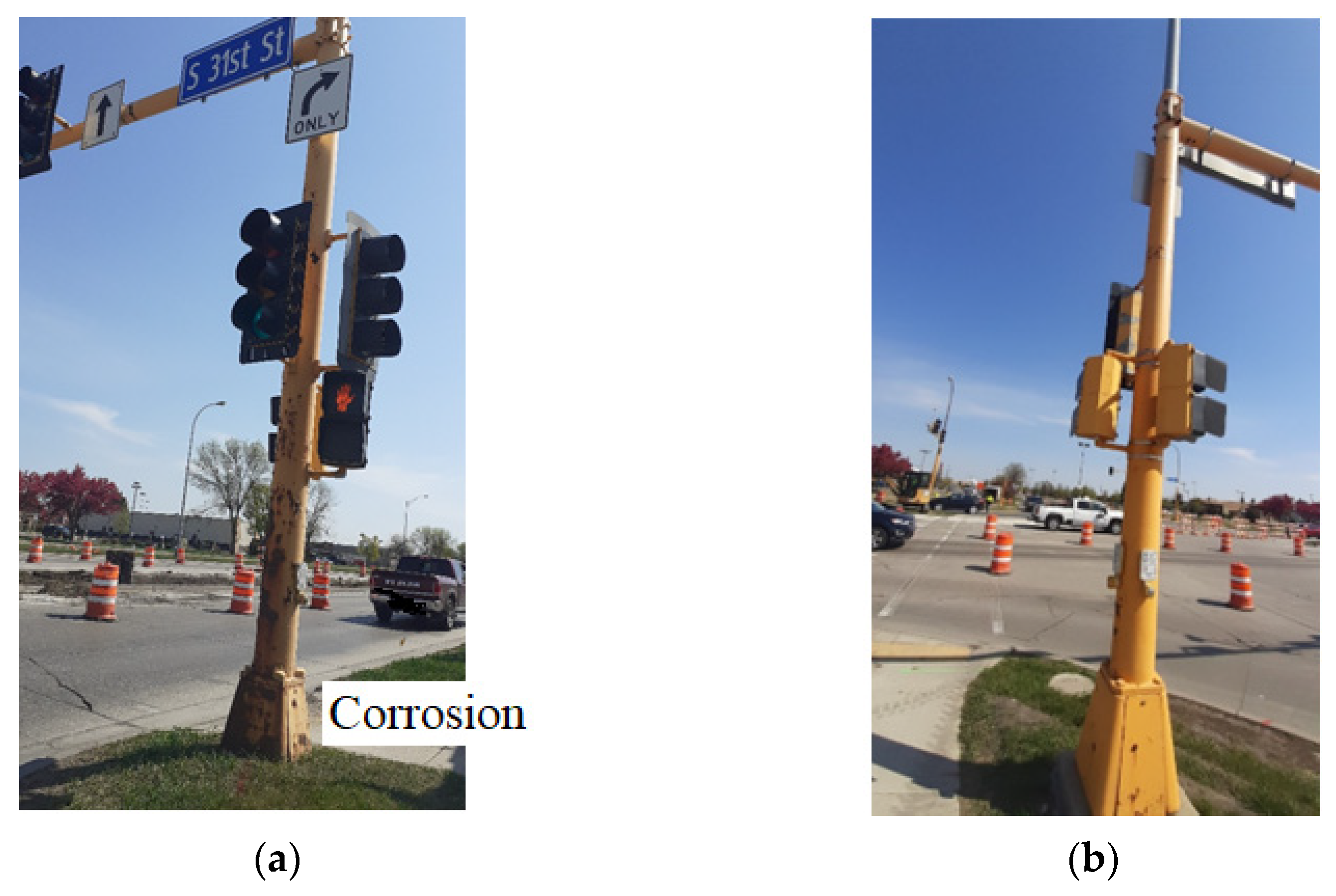
Figure 1a,b illustrates images of an existing ancillary structure in Grand Forks, ND, exhibiting significant corrosion and without visible corrosion, respectively.
Corrosion significantly affects the overall cost of steel structure maintenance [7], and if neglected, can lead to section loss and eventual failure. For instance, the corroded ancillary structure shown in Figure 1a was replaced due to severe corrosion to avoid continuous deterioration and subsequent failure. A total of 42% failures of structural elements occur due to corrosion of steel structures [8]. Moreover, continuous contact with water or electrolytes could cause internal corrosion in the case of tubular members [3].
The hands-on inspection technique has certain drawbacks [9] that create the need for computerized digital image recognition, a feasible alternative regarding safety, efficacy, consistency, and accuracy. Despite the advantages of the currently practiced NDE technique in the inspection of steel structures, the automated optical technique is the most preferred due to its simplicity in use and interpretation [6,10,11]. This usually involves the onsite acquisition of digital images of the structure, followed by an offsite analysis using image processing techniques for corrosion detection [6,12]; however, there have been some attempts for real-time processing [13,14].
Researchers have proposed various image processing techniques to detect steel structure corrosion [7,8,
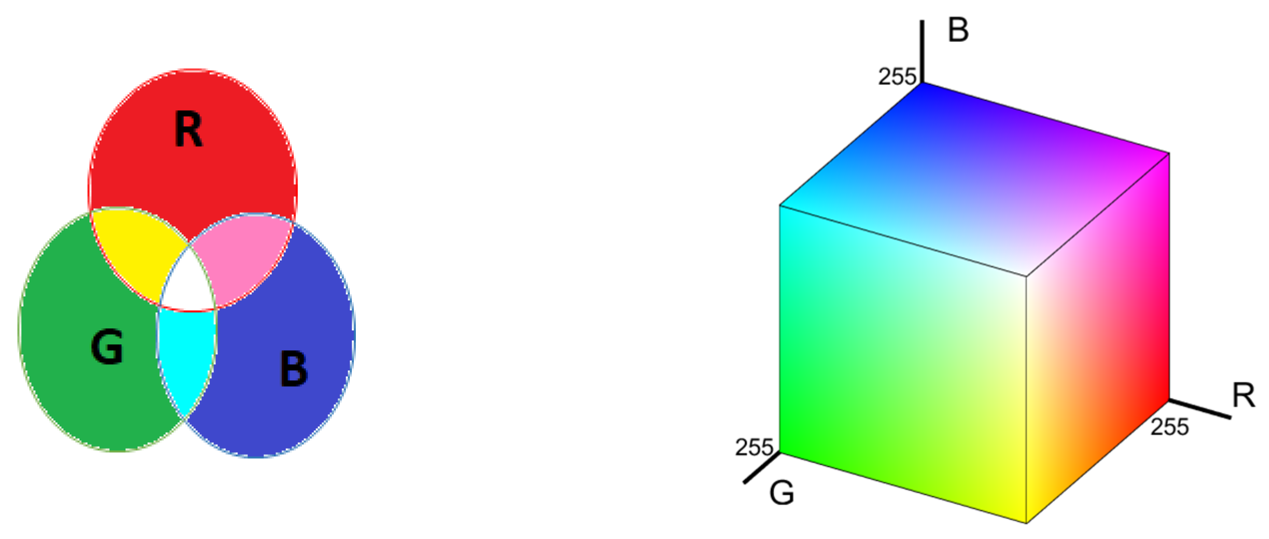
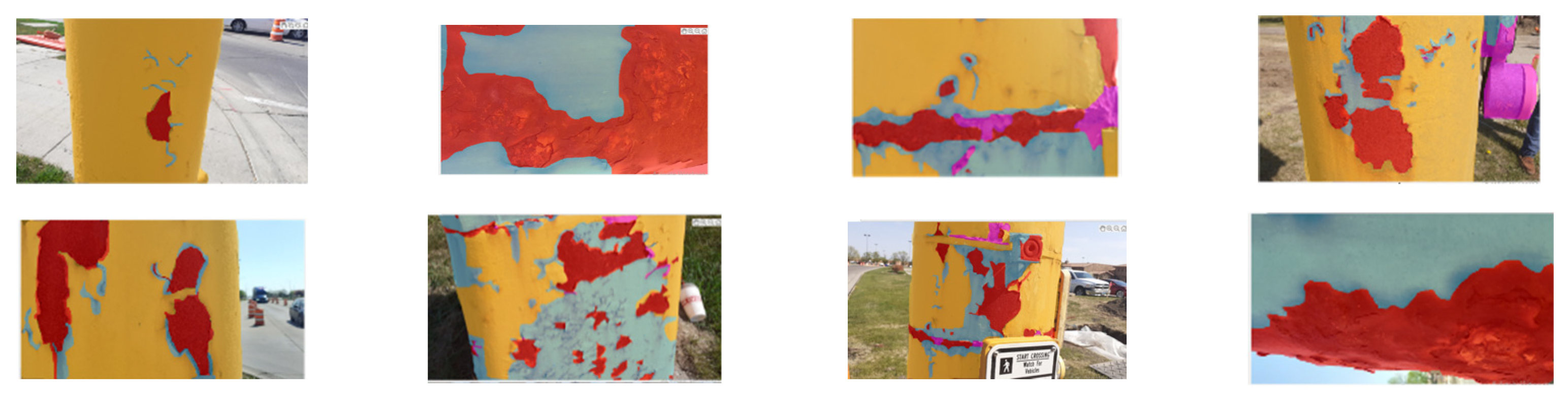
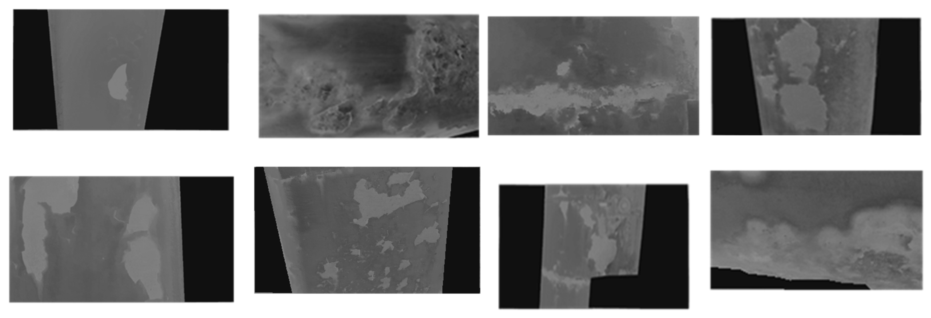
15]. The texture analysis technique characterizes the pixels of images for classification problems. Pixels associated with corrosion in visual images of ancillary structures have a rougher texture and a distinct color compared to noncorroded or sound pixels. Here, color and rough texture are considered features for pixel classification. Past research studies have investigated corrosion using RGB (red, green, blue) color space without considering the presence of undesired objects in the image’s background [12,16]. Most studies have either evaluated corrosion without corrosion quantification from ground truth or have used images collected under controlled environments [6,7,8], as these image-based algorithms are usually affected by undesirable illumination presence of the background.
The state’s Department of Transportation (DOT) commonly performs corrosion detection inspections using visual and physical methods. The primary goal of this research is to develop an automated adaptive image processing-based algorithm to detect the corrosion of in-service ancillary structures under ambient environmental conditions. In addition, actual onsite conditions of ancillary structures, such as background and natural lighting, were considered while processing the data.

2. Overview of Corrosion Detecting Sensors

There are numerous nondestructive techniques for corrosion detection. Fiber Bragg grating (FBG) sensors are used to evaluate coated steel’s corrosion behavior [17]. The performance of electrochemical tests and FBG sensors was compared. Two types of coating—polymetric and wire arc-sprayed Al-Zn (aluminum-zinc) coatings—were used to verify the FBG sensor’s performance. Finally, it was shown that FBG sensors perform well for both detecting corrosion and crack initiation. In past studies, researchers found ultrasonic sensors to be one of the most effective devices for corrosion detection [18,19], but they required expertise to identify the critical location of corrosion. Again, an optical microscope was used to detect the hidden corrosion of depths 0.02 to 0.40 mm in steel plates [18].
Moreover, the traffic lane may need to be closed as these methods need contact with the investigating structural element. Corrosion identification using image processing methods can address both limitations. Digital cameras collect the digital data necessary for image processing methods. However, the sensor type and number specified for data collection are not constant in all inspections. Visual and thermal cameras are the most widely used sensors for corrosion detection and structure evaluation due to their availability, even though other sensor types can perform corrosion assessment and evaluation [12]. In addition, these sensors can be mounted on an unmanned aerial vehicle/system (UAV/UAS) [9], which does not need the closure of a traffic lane, as well as auxiliary arrangements such as a ladder and other detection instruments.

3. Color Spaces and Image Processing Techniques

3.1. Color Spaces

The human eye or camera sensor can detect light incidents when reflected off a material. The beam of light that reaches the eye or camera is the interactive result between the distribution of the light source’s spectral power and the target’s spectral reflectance. The formation of color into a signal can be described by the following Equation (1) [20].
    f c ( x ) = ω   E ( γ , x ) ρ c ( γ ) d γ
Here, fc (x) is the measured observation value; E(γ,x) is reflected energy from the surface, where γ is the wavelength and x is the spatial coordinate of the image; and ρc is the camera sensitivity, where c∈ {R, G, B} and ω is the visible spectrum. R, G, and B are red, green, and blue, respectively. Understanding color space is necessary to develop digital image processing models and properly develop color image processing methods. According to colorimetry, each color is a combination of three color coordinates. Commission Internationale de l’éclairage (CIE) introduced color space by mathematical formulas [21]. Again, color is defined as the portion of EM (electromagnetic) radiation seen by humans [20]. The wavelength band ranges from approximately 380 nm to 740 nm. The color images contain more detail and information than grayscale images [22]. Some of these details are chromaticity and luminosity. Chromaticity refers to color classification based on its deviation from white light, also known as hue and purity. The luminosity parameter measures the hue’s degree of brightness or darkness. Color spaces can be of different types: RGB (red, green, blue), HSV (hue, saturation, value), HSI (hue, saturation, intensity), L*a*b (luminosity, red or green component, yellow or blue component), YCbCr (luminosity and combination of chrominance component). In this study, two color spaces, RGB and YCbCr, were considered. RGB is the conventional color space for visual imaging. On the other hand, it is revealed that human vision is more sensitive to the luminance component; therefore, it becomes more efficient to represent images in YCbCr form. A concise explanation of these two color spaces is mentioned in the following sections.

3.1.1. RGB Color Space

RGB color spaces are primarily composed of three color bands. The intensity value ranges from 0–255 for each band. A combination of all color bands at the same intensity results in white color (255,255,255); however, the absence of all color components results in black color (0,0,0). The brightness of the same color can be modified by manipulating the color components using a constant multiplier or quotient [23]. The origin of the RGB color space is represented in a 3D cube in Figure 2, with values ranging from 0–255.

3.1.2. YCbCr Color Space

The Y component of the YCbCr color transformation space depicts the luminance component, a measure of light intensity. The Cb and Cr components represent the chrominance component, which measures the green component with respect to the blue and red component intensity differences [24]. The most important feature of the YCbCr model is that it imitates human vision, which responds to light intensity changes more than hue changes [25]. Therefore, the Y component has a range of [16–235], while the Cb and Cr components have a range of [16–240] [25]. Figure 3 illustrates the transformation of captured images from RGB to YCbCr color space. As can be seen in Figure 3, pixels associated with corrosion are more pronounced in the YCbCr color space. The mathematical equation for this transformation will be introduced later in this paper.

3.2. Image Processing Techniques

Routine corrosion detection is vital to ensure ancillary structure integrity. However, conventional physical and visual methods are used with inspection aids such as ladders or scaffolders to gain access to difficult parts of the structure. Image acquisition using UAS combined with image-based corrosion detection algorithms is an alternative solution that can increase accuracy and robustness without lane closures [9]. Moreover, image processing techniques using an automated inspection system are timesaving and less tedious than visual inspections [26,27].
Collecting quality image data is a crucial step for obtaining reliable evaluation results. Image data using UAS can be collected using hand-held or mounted sensors or other data collection platforms. In texture analysis, a rough area was categorized as a corroded region performed on the images captured by a camera with a resolution between 12 MP–18 MP [7,28]. Again, UAS can be integrated with image processing techniques for large steel structure corrosion detection with intelligent obstacle avoidance, positioning, stable hovering, and other flight characteristics [29]. Non-contact-based thin steel film electrical resistance (TFER) is another technique developed to detect corrosion by measuring the change in the sensing element’s electrical resistance [30]. The k-means clustering algorithm was used to extract the region of interest (ROI) from the images of pipelines in a subsea environment by grouping the corroded pixels of different intensities [31]; however, the mean reported accuracy was 90%. To improve the result of conventional image processing, different preprocessing steps such as the change of color space, applying filters, and morphological operators play significant roles [6,32,33]. The transformation of color space might help to segregate the background from the foreground with the same color [32]; however, the L*a*b color space proved better among the 14 color spaces used for conversion. Again, the use of Fourier transforms together with image processing steps was found to be most effective in cyan (C), magenta (M), yellow (Y), or CMY color spaces, with about 99% accuracy for corrosion detection [33]. Some researchers have focused on developing a relationship between the statistical features of sound and defective images [26,34]. A rust defect detection method (RUDR) was designed to analyze corrosion detection images comprising data preparation, analysis, statistical modeling, testing, and validation. The images were preprocessed prior to the main processing. The preprocessing step evaluated the presence or absence of defects in each digital image. The image was further processed and evaluated if found to be defective [26].
On the other hand, the combination of k-means clustering and statistical parameters was adopted for corrosion detection. Mean, median, skewness, and textural parameters in the HSI color space were used to segment microscopic corrosion images with 10 pixels by 10 pixels, yielding 85% accuracy [34]. The similarity index is also used for corrosion recognition using color and texture features extracted from the images [35]; the images with a similarity index less than one are defined as defective. Finally, pixels are compared with the corrosion color spectrum. Pitting corrosion had also been detected in pipelines using a support vector machine (SVM)-based machine learning model, yielding an accuracy rate of 92% [8]. On the other hand, 67–90% corrosion detection accuracy was obtained from the fully trained artificial neural network from the images transformed into four different color spaces [6].
Past research shows that images used for corrosion detection were free of artifacts and collected under controlled lighting conditions. Therefore, artifacts such as background were not excluded from the dataset, unlike other studies where the datasets are clean and do not depict the actual onsite condition of structures. At the time of preprocessing, the brightness of the images was modified accordingly. The model’s performance was validated using images captured by a camera mounted on the UAV. Removal of the background is an essential step in preprocessing. In most studies [6,7,8], model performance was evaluated by determining only the conventional performance metrics. In this study, image quality metrics were also considered as model performance evaluators. Furthermore, the proposed method will enable the inspector to exclude the image’s background, making it a possible and effective method for real-time inspection.

4. Dataset Generation and Processing

4.1. Image Data Acquisition

A cellphone camera was used to capture 300 images from four in-service traffic poles located in Grand Forks, North Dakota, on 17 May 2021, between the hours of 10 a.m. to noon. The poles had an average height of 7 m and a cantilever arm length of 6–7 m. This mobile phone had phase detection autofocus (PDAF) technology designed to mimic human eyes by pairing masked pixels on the image sensor. Examples of images collected are shown in Figure 4. The specifications of the camera used are summarized in Table 1. The sizes of the images are 2322 pixels by 4128 pixels. The images were collected for differing degrees of corroded and sound regions showing different background scenes in the image. In addition, the data were collected considering the traffic to ensure the safety of inspectors.
Another set of image datasets was collected in Fargo using a UAS equipped with a visual camera to verify the model’s performance with respect to image quality. The ambient weather condition for temperature, humidity, and wind speed during data collection is shown in Table 2 [36].

4.2. Data Annotation

Images were annotated using an image labeler app in MATLAB R2020a image processing toolbox. All computations in this study were performed on a desktop computer with a 64-bit operating system, 16 GB memory, and a 2.9 GHz processor running an Intel ® Core™ i7-10700 CPU. The annotated images were used as ground truth for benchmarking the input images. As shown in Figure 5, all images were labeled into two classes: corroded and non-corroded. A total of 95,539,808 pixels of these categories were annotated for each image. Depending upon the severity of corrosion, a range of 2.5 to 64.5% of the pixels of the images were annotated as corrosion with red, blue, and pink colors. The different colors represent the different severity of corrosion. The remaining portion was considered as background pixels. Since the determination of the corrosion scale was way beyond this paper’s scope, all images were converted to binary images (pixels with and without corrosion) and used as ground truth for further analysis. This semantic segmentation method is known as a dense prediction, as it predicts the class of each input pixel with respect to the assigned class.

4.3. Scene Constraints and Preprocessing

In developing a robust and viable algorithm for corrosion detection, existing environmental constraints play a crucial role. For instance, sunlight reflection could cause some portions of the region of interest to have high brightness, while other parts could be under the shadow; illumination plays a vital role in image quality. The illumination of all the images was modified by developing an algorithm to increase the proposed algorithm’s success. All the original images were preprocessed by converting them to the YCbCr color space to control the luminance. In addition, varying objects on the image background could challenge the ease of corrosion detection. Though the corroded part had prominent color, sometimes the background color created complexity. The existing site constraints and surrounding objects were captured in the background during data collection. Since these were field data, the researchers had no control over these constraints appearing on the image’s background. Dey [37] discussed the effect of uneven illumination and concluded that noise due to external interference and imbalanced illumination is a typical image-related artifact during image acquisition. In addition, the uneven distribution of light could have been caused by the presence of large objects in the image’s background [38]. They also mentioned that the presence of other objects’ shadows makes it challenging to optically segment and isolate the object of interest. The constraints resulting from illumination variations and the presence of undesired objects in the background make conventional segmentation techniques ineffective in corrosion detection for small objects. Moreover, an unsupervised segmentation technique can produce unreliable results in the presence of noise components, shadows, and reflections from light sources.
A preprocessing algorithm was developed in this study to increase the quality of the collected images for corrosion detection. Some image enhancement steps followed the preprocessing operation. In this step, contrast adjustment and histogram equalizations were used to distribute the pixels uniformly or eliminate noise from the image. First, the contrast was adjusted to improve the output image quality, resulting in 1% of the pixel values being saturated at high and low intensities. Here, saturation implies remapping pixel values in a low-contrast grayscale image to fill the entire intensity range [0, 255]. After the contrast adjustment, the input image’s histogram was equalized using Equation (2) to ensure uniform distribution of pixels’ intensities [16].
c ( I ) = 1 / N i = 0 I h ( i )
where N is the number of pixels in the image. Here, c(I) is the cumulative distribution from the integration of the histogram of the original image, h(I).
Finally, all the pixel values were redistributed using adaptive histogram equalization, which differs from histogram equalization. In the adaptive method, several histograms were computed for the images. Finally, the output image shows improved contrast and a more visible edge than the input images. Figure 6 shows corroded images before and after preprocessing. Corrosion is seen to be more visible in the preprocessed images than the raw images, since the presence of shadow or uneven illumination have been minimized in the final image.
The change in brightness as a result of the preprocessing is computed from Equations (3)–(5) [39]. If R′, G′, B′ is the normalized value of the R, G, B image for the standard RGB color space (sRGB), the relative luminance(Y) can be defined as Equation (3).
Y = 0.2126 × s R + 0.7152 × s G + 0.0722 × s B
Here, sR can be determined from Equation (4).
s R = {   R 12.92                   i f     R 0.03928 (   R + 0.055 1.055 ) 2.4 O t h e r w i s e                                    
Similarly, sG and sB values can be determined from Equation (4) by replacing R′ with G′ and B, after which the brightness (L*) of the image can be calculated from the following Equation (5).
L * = { Y × 903.3                                   Y 0.008856 Y 1 3 × 116 16       Y > 0.008856
Since the brightness of images plays a significant role in detection accuracy, the performance of the model was verified by testing on another dataset. The dataset consists of images without corrosion and UAV payload images. The images without defects will be mentioned as sound images in all the text later. Moreover, image quality has an enormous impact on the result of image processing techniques. Quality metrics such as the Blind/Referenceless Image Spatial Quality Evaluator (BRISQUE), Natural Image Quality Evaluator (NIQE), and Perception-based Image Quality Evaluator (PIQE) have been determined for the images [40,41,42]. In this case, sound images are used as reference images. The quality metrics were used to detect possible poor images after the preprocessing.

4.4. Artifact Reduction from Images

Except for the issues related to illumination, the presence of undesirable objects as background could affect the performance of the corrosion detection model. A computationally light framework for the user was developed to subtract the background from each image. At first, the boundary was drawn by a polygon around the background. Afterward, a binary mask was generated, where nonzero pixels were for the background and zero pixels were for the region of interest. In the next step, the background was subtracted from the input image. By completing this step, the region of interest was separated from the background. Finally, the input image was overlaid on the binary image (Figure 7). After overlaying, the background color turned yellow by default. The novelty of this algorithm is that in real-time, the inspector can subtract the background to explore their desired inspection location. Color space transformation is the next step implemented on these images.

4.5. Color Space Transformation

The proposed approach transformed the captured images in RGB color space into YCbCr color space. Afterward, the transformed images were split into three different components (channels) based on luminance and chrominance. Equation (6) shows the transformation matrix [25]. Corrosion was expected to be more pronounced in the Cb component, and therefore segmented more conveniently. Finally, the color threshold app of MATLAB image toolbox was used for the thresholding to extract the foreground (object) from the background. Figure 8 and Figure 9 show images in YCbCr color space and corrosion detection of images shown in Figure 4.
[ Y C b C r ] = [ 16 128 128 ] + [ 0 279   0 5040 98 0 148 0 2910 439 0 439 0 368 0.071 ] [ R B G ]

4.6. Binarization

4.6.1. Otsu Threshold Method

In this process, each pixel in the image is placed in one of two classes. One class contains pixels within the region of interest; the other contains pixels not in the region of interest. In this step, corroded pixels are labeled as one and the remainder as 0. Binarization is an essential step in image processing. The binary image is used afterwards to build a set of parameters for classification. Successful binarization depends on the selection of the threshold value. This method can determine an optimum threshold by minimizing the weighted sum of variance between two classes: background and foreground. The colors in grayscale vary from 0 to 255. The binarization process can be described by Equations (7)–(10) [43]. At any threshold t, the variance between two classes (σ2) is evaluated by Equation (7):
σ 2 ( t ) =   ω bg ( t ) σ 2 bg ( t ) +   ω fg ( t ) σ 2 fg ( t )
ω bg ( t ) = P bg ( t ) P all
ω fg ( t ) = P fg ( t ) P all
The variance can be calculated using the formula below:
σ 2 ( t ) = ( x i x mean ) 2 / N 1
where x_i is the value of the pixel at i in the group (bg or fg), x_mean is the mean of pixel values in the group (bg or fg), and N is the number of pixels.

4.6.2. Global Threshold Method

A threshold value should be selected in a way that would suppress the background while leaving the corroded pixels visible. A low threshold value will create noisy pixels that can distort the features, introduce extra features, and increase the complexity of the analysis. The Otsu method selects the threshold value automatically, whereas in the global threshold method, one arbitrary number is used for the whole image. In this study, we developed an iterative algorithm by evaluating the relationship between the threshold value and the performance metrics rather than choosing an arbitrary threshold value. The model was evaluated with the performance evaluation metrics: (i) accuracy (ACC), (ii) positive predictive value/precision (PPV), (iii) F1-value, (iv) sensitivity/recall/true positive rate (TPR), (v) specificity/true negative rate (TNR), (vi) false-positive rate (FPR), (vii) false-negative rate (FNR), (vii) intersection over union (IOU).
The metrics are calculated by the following Equations (11)–(15):
A C C = TP + TN TP + FP + TN + FN
F 1 S c o r e = 2 TP 2 TP + FP + FN
T P R = TP TP + FN
T N R = TN TN + FP
I O U = TP TP + FP + FN
Here, TP means correct detection of the corroded pixel and TN means correct detection of sound pixels. On the other hand, FN and FP are opposite to TP and TN, respectively. ACC is the rate of correct corrosion detection for the total detections. The PPV and TPR provide helpful information about the prediction outcome. TPR gives the fraction of actual corrosion that the model correctly detects. Lower TPR rates indicate a high number of false negatives. All the performance metric parameters are determined with respect to the ground truth. Figure 10 shows the representative relationship between the threshold value and performance metric elements. The point where all the curves for each performance metric element meet can be termed an intersection point. The intersection points for all other images were also determined and used as the base threshold value for binarization.

4.7. Morphological Operations

The output of the proposed image processing method is a binary image that includes one or more connected components segmented as corrosion (Figure 11). However, most semantic segmentation techniques suffer from residual misclassification, generally manifested as more minor discontinuities in the binary image. Morphological operations can manipulate the shape and size of connected components in binary images. They are commonly used in texture analysis, noise elimination, and boundary extraction [44]. Morphological operation is applied using a small template called structuring element (se). The structural element is applied to all possible locations of the input image and generates an output image with the same size as the input. The operation’s output produces a new binary image with a non-zero-pixel value at that location if the operation is successful. There are different structural elements, such as diamond shapes, lines, disk shapes, circles, and spheres. Conventionally, opening and closing operations are performed on binary images. This study performed opening and closing operations with disk-shape structural elements on the RGB images after the illumination modification. Since the dimensionality of the RGB image is greater than that of the structural element, this morphological operation worked along each channel. In this step, any artifacts from processed images were removed. After binarization, a line-shaped structural element with a length of 20 at an angle of 180 degrees denoised the binary image more than the disk shape. Therefore, it is better to apply the morphological command after defining the boundary of the region of interest. In this study, all the detected edges bridged other regions for extracting the target area before implementing the morphological operations (Figure 12).
If morphological opening is γ s ( A ) and morphological closing is β s ( A ) , then from Equations (16) and (17) [45]:
γ s ( A ) = ( A   $ ) $
β s ( A ) = ( A   $ )   $
Here, A is the binary image, and $ is the structural element of the desired shape and size. In this work, $ is a line-shaped structural element with a length of 20. ⊖ and ⊕ operators are used for erosion and dilation, respectively. $′ is the transpose of $.
Dilation also transforms the images with a change in size. This operation stretches or thickens the region of interest by bridging the gaps between pixels [41]. Dilation can remove negative impulsive noises. The dilation of A by the structuring element $ is defined by Equation (18) [45]. Here, Ac denotes the complement of A.
A $ = ( A c $ ) c  

5. Results and Discussion

5.1. Brightness and Image Quality

The novelty of the proposed method is the brightness modification of the test images at the preprocessing stage. This step is followed by background removal, color space transformation, and corroded pixel detection rate determination. From the results presented in Table 3, it is found that in comparing the processed and preprocessed images, the brightness change is not beyond 10%. This implies that the proposed model did not change the brightness of the images unnecessarily to change the image quality.
The same sound images were used for quality check. From the reported values of quality metrics in Figure 13, it was found that after preprocessing, all values decreased. The average reduction in BRISQUE is 21.5%, while for NIQE and PIQE quality metrics, the reduction rates are 10.53% and 37.53%, respectively. This implies that the quality of the images improved with the brightness modification.
A comparison of images in the original and preprocessed conditions is presented in Table 4. In Table 4 and Table 5, all the brightness values in candela(cd) of different images are presented. Further investigation was performed on the influence of preprocessing on the TPR and TNR values. From the result, it is reported that brightness change did not significantly affect TNR values. On the other hand, a change in brightness above 10% reduced the correct detection rate up to 20%. The brightness of all the images except images 5 and 8 changed by less than 10%; the corroded zone segregated from the sound part more clearly. For example, in image 3, the right corner portion of the image was overexposed to the sun; therefore, the corroded part became blurry. After preprocessing with a 2.32% brightness increment, all the corroded parts became prominent, which finally led to a 9% increment in TPR value. The highest increment in TPR value happened for image 4, which is 20% with 3.5% brightness modification. The reason behind this significant increment can be justified by the binary image presented in Table 6.
The preprocessing steps included the conversion to the YCbCr color space, which was found to be better for the separation of a corroded part from the background. Moreover, proper extraction of the corroded region from the sound part helped in denoising. On the other hand, the TPR value decreased by 20%, with a 16.5% increment in brightness for image 8. From Table 4, it is clear that after the preprocessing steps, color modification of the sound portion took place, and thus due to the similarity in color, the model predicted these as false positives. The change in brightness after preprocessing is determined with respect to the original image; a negative sign implies an increment after preprocessing. On the other hand, a negative sign for TPR changes means a decrement in correct detection with respect to the original image.

5.2. Optimum Threshold and Morphological Operators

In this study, both the Otsu and global threshold methods were used for image binarization prior to preprocessing. For the global thresholding method, the threshold value was not selected randomly. The value of the performance metrics for 0 to 1 threshold value with increment 0.01 have been determined for each image (Figure 10). For all images, there was no common intersection point for the plotted curves. The summation of the true positive and true negative was determined for each threshold value (Figure 14). From the comparison of Figure 10 and Figure 14, it can be deduced that at the intersection of the curves, as the TPR value increased, the TNR decreased significantly. For example, most of the performance metrics curves reached it’s peak at threshold value 0.6. However, in Figure 14, it is depicted that the correct prediction rate of the sound pixels decreased by around 0.6. The selected threshold value ranged from 0.27–0.52 for the images. Beyond this range, the summation of TPR and TNR drastically dropped. In general, the Otsu and global threshold methods work better on the images with bimodal histograms. Since the tested images are with different scales of corrosion, the pixel intensity distribution would not be bimodal. From Figure 14, it is evident that TPR+TNR-values change even with a 0.01 increment in the threshold value. All the performance metrics related to each threshold method are reported in Table 7. From the result, it is found that Otsu reduced the overall accuracy of the model by 20%; therefore, global threshold values were adopted for the binarization of the preprocessed images. After extracting the connecting edges, a dilation operator was implemented with line-shaped structural element size 20- and 180-degree angles. This is the optimum value for both size and angle. False-positive detection was higher with the increasing size.

5.3. Performance Metrics

In Figure 15, all the relevant parameters of performance metrics are presented for both the original and preprocessed images. From the results presented in Figure 15, TPR and accuracy are seen to have increased for all represented images except for images 5 and 8. The rate of increment for each image varies from 10 to 20%. The average TPR value for all preprocessed images was about 66%, whereas this value was 56% for the images without preprocessing. Among the investigated images, the corroded areas with uniform illumination and without undesired objects were categorized with an average true positive rate of 70%, whereas for uneven images, it is around 60%. The reduction in corrosion detectability in images 5 and 8 could be due to the loss of some features in the image during illumination modification, such as the increment in brightness. The reported brightness increment is 14–16% for these two images, which is beyond the optimum value. On the contrary, the proposed algorithm increased the accuracy and true positive rates by 7–10% for the preprocessed images. The average TNR value for preprocessed images is 90%, whereas it is 84% for images without preprocessing. These values indicate that the model successfully detected the sound pixels. The overall rate of accuracy for the preprocessed images was 90%, whereas for the original images it was about 77%. Similarly, the F1 score considerably increased from 60% for the unprocessed images to 67% for the preprocessed images. The mean IOU increased from 46% to 57.3% after preprocessing of images.

5.4. Efficacy of Proposed Method

5.4.1. Comparision with the Previous Method

The authors adopted the methodology proposed in the previous study in [15]. The researchers in [15] acknowledged that they had intentionally ignored the background for the sake of easiness of model development. On the other hand, a background removal algorithm was incorporated by the authors in this study. After comparing two methodologies, it has been revealed that the proposed methodology detected 23% more corroded pixels than the method mentioned in [15] when the image had background. However, the proposed method showed its superiority, with 11% more correction detection, even with the images with very negligible background. The results are presented in Table 8.

5.4.2. Robustness of Model Irrespective to Dataset

The robustness of the proposed model was evaluated qualitatively on several images collected by UAS from in-service ancillary structures. From visual scrutiny, it was confirmed that the model was capable of segmenting the corroded pixels from the background at large. In addition to this, it is worth mentioning that these test images were not used during model development as they were collected after the model was developed. Results are presented in Table 9.
Though the proposed model proved its supremacy with respect to the previously used method and external datasets, it had some limitations. The effect of different lighting conditions was not considered for developing the brightness modification algorithm. As a result, the generic modification of brightness did not work as expected for all the images except for the overexposed images. Background removal was another cruical step in the proposed preprocessing steps. As a first step of background removal, a boundary was drawn by a polygon around the background. Since it is drawn manually, leaving out any background pixel can cause a false prediction. Like the other image processing method, the threshold value for binarization needs to be defined, which might hinder the autonomy of the model to some extent.

6. Conclusions

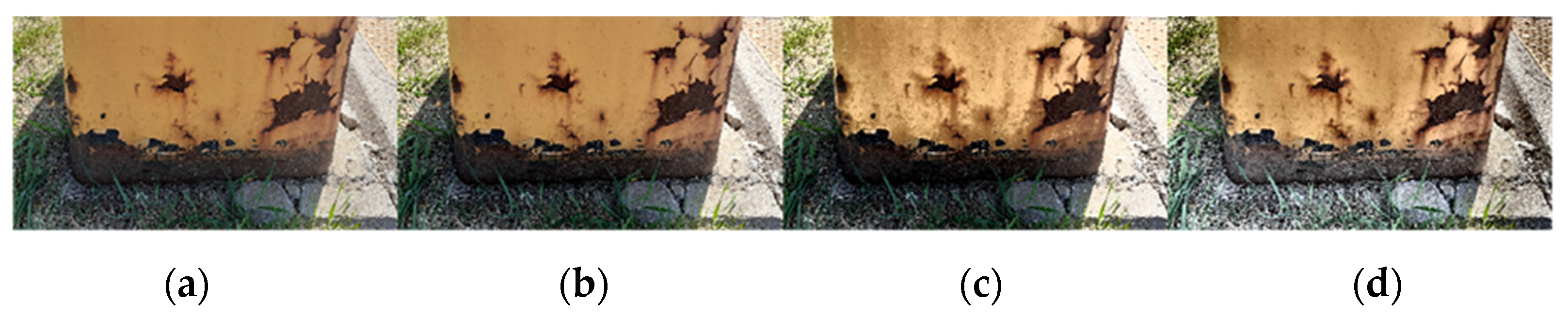
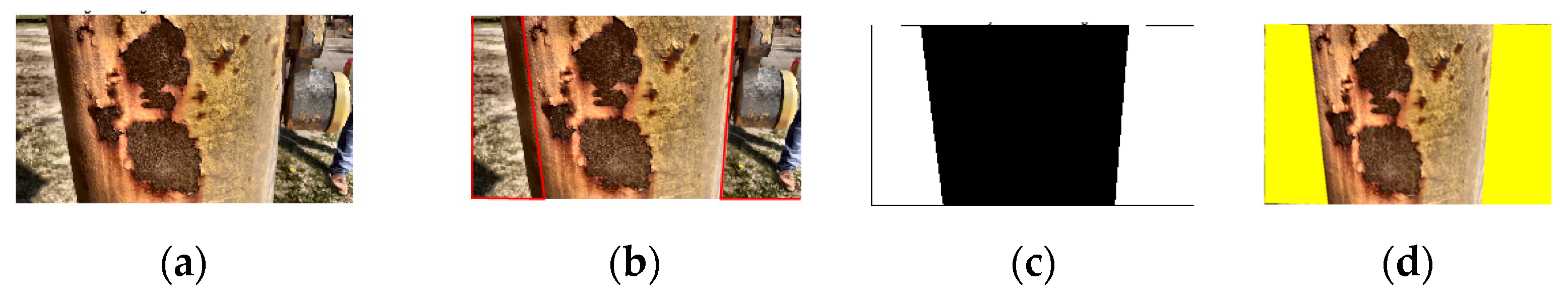
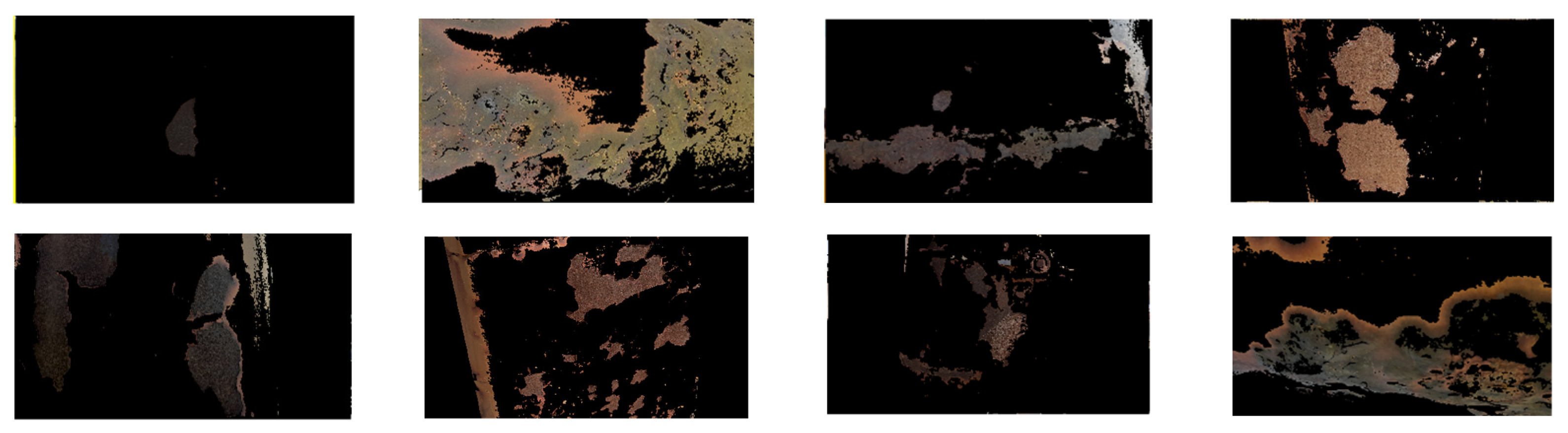
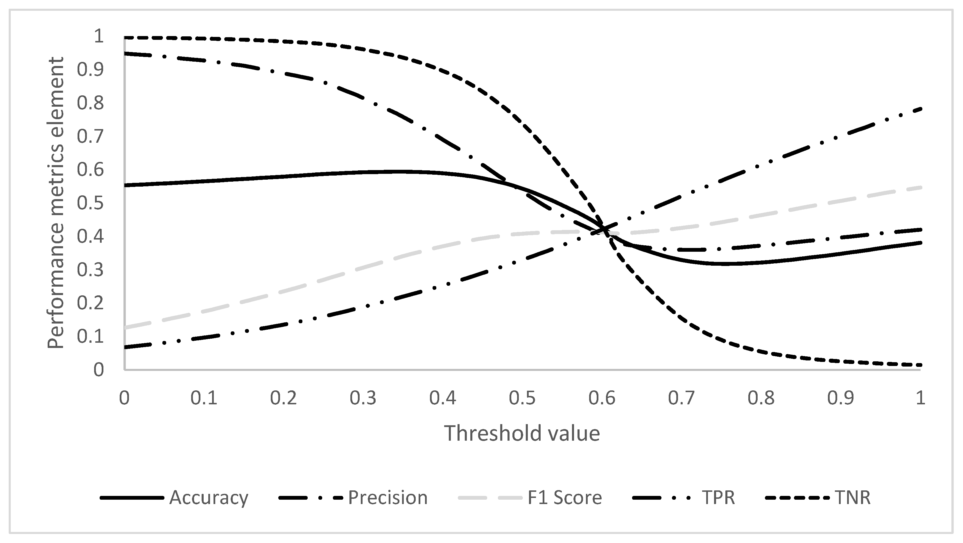
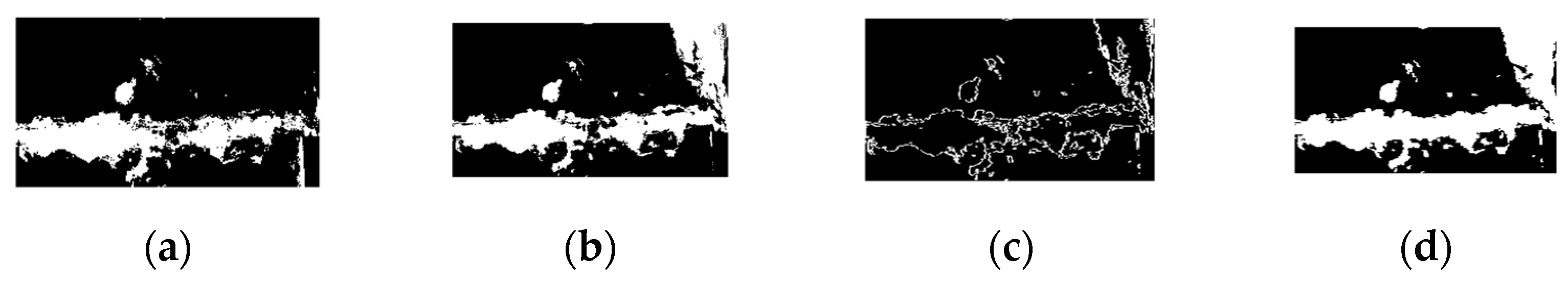
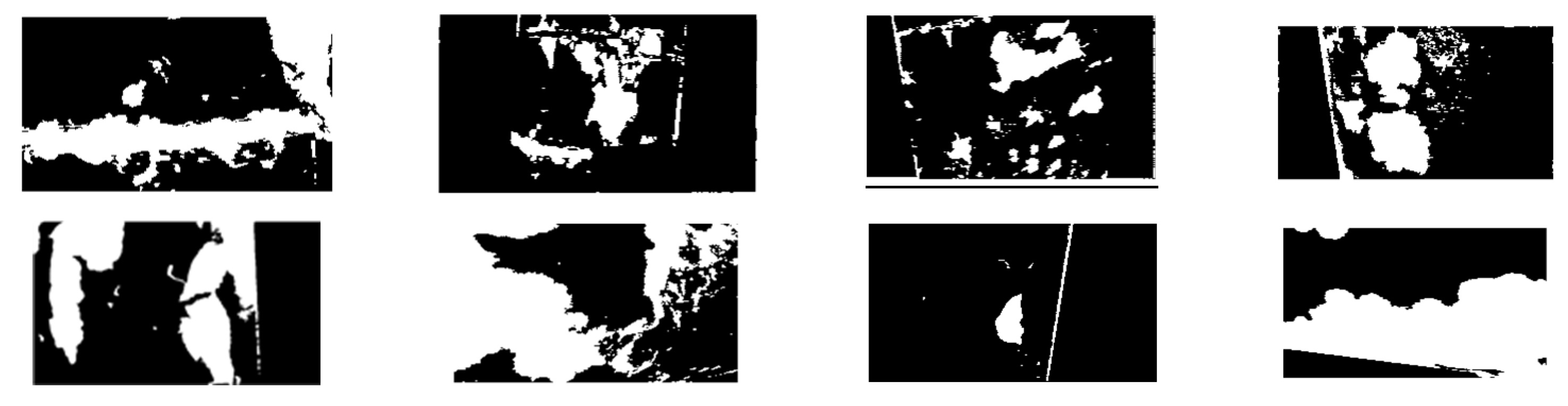
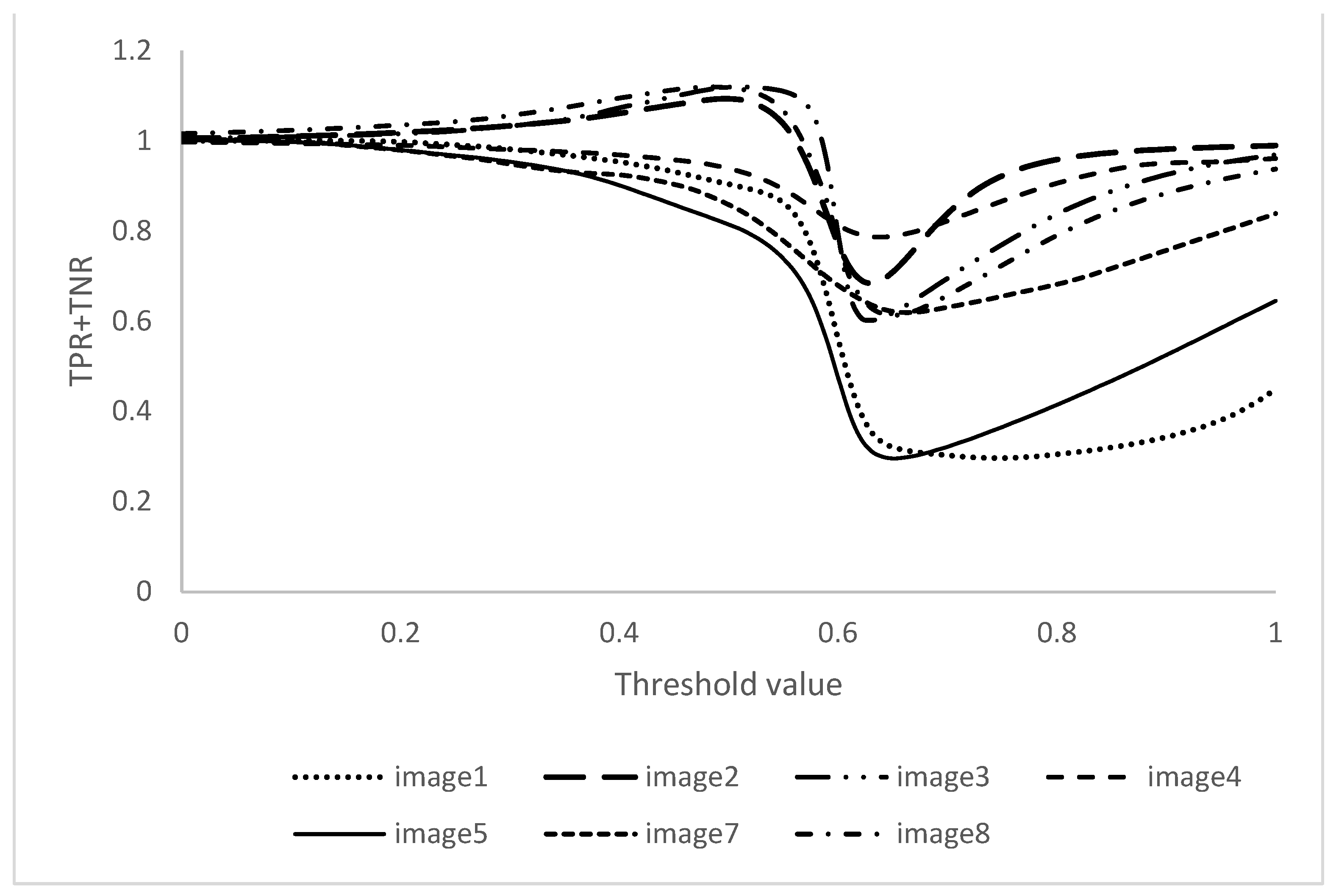
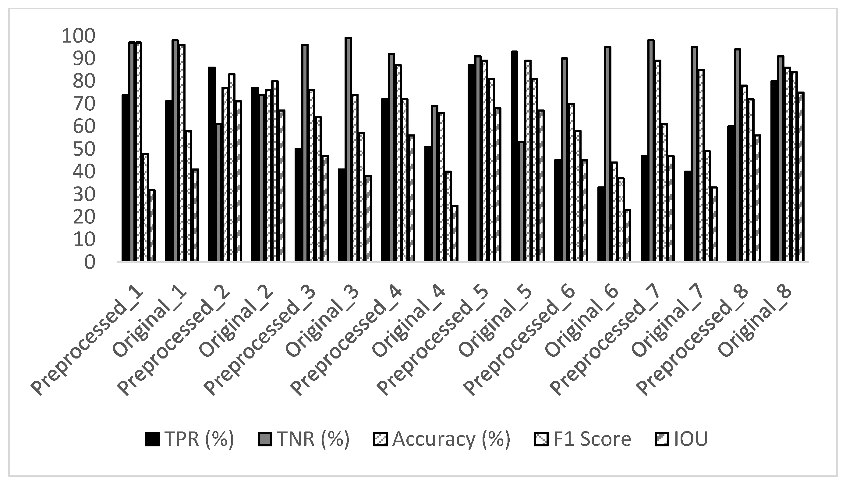
This study presents a novel image-based technique to detect corrosion in ancillary structures. The model was evaluated on sets of images with and without preprocessing. The maximum 20% TPR value improved after the preprocessing steps, followed by background removal and color space transformation. However, the brightness modification should be within the optimum range. Among the investigated images, the corroded areas with uniform illumination and without undesired objects were categorized with an average true positive rate of 70%, whereas for uneven images it was around 60%. Regarding the threshold method, optimization of the threshold value with respect to the performance metrics showed better results than Otsu.
The efficacy of the developed model was evaluated in two different ways: comparison with previous method and tested on external images. In comparison with the previous method, the proposed model detected 23% more corroded pixels correctly from the images with background. Qualitative results of the proposed model on the external images are also promising.
The study revealed that several factors, such as the presence of background objects, preprocessing, color space used for processing, image quality, and thresholding values, affect the performance of any conventional image processing model. Several of these shortcomings have been investigated and addressed through the proposed methodology. The results from this study show significant promise for the future adoption of autonomous unmanned aerial systems and artificial intelligence methods for image-based corrosion monitoring and detection in ancillary structures. Limitations of the proposed image-based algorithms include the selection of the optimum threshold value for binarization, generic brightness modification, and the need for background removal. Deep learning semantic segmentation models in combination with image processing methods could be considered for future work to develop a robust corrosion detection model to combat this limitation.

Author Contributions

S.D. and A.D. both conceived and designed the methods; A.D. and E.I. collected the data on the field; A.D. performed the preprocessing, image processing, annotation, and storage of the dataset; A.D. developed the corrosion detection code. A.D. and E.I. prepared the manuscript, and S.D. reviewed the paper; S.D. acquired research funding and supervised the research. All authors have read and agreed to the published version of the manuscript.

Funding

This research was funded by the North Dakota Department of Transportation (NDDOT) for the project “Smart UAS Inspection of Ancillary structures in North Dakota” under fund number UND0025168.

Data Availability Statement

Data are available upon request to the corresponding author.

Acknowledgments

We wish to thank the entire staff and management of NDDOT for helping realize the project’s goals and objectives. The finding of this paper does not reflect the official views of NDDOT. We also extend our gratitude to Anna Crowell and Dayakar Naik Lavadiya for their help in editing.

Conflicts of Interest

There are no known declared conflict of interest.

References

  1. Kaczinski, M.R.; Dexter, R.J.; Van Dien, J.P. Fatigue-Resistant Design of Cantilevered Signal, Sign, and Light Supports; Transportation Research Board: Washington, DC, USA, 1998; Volume 412. [Google Scholar]
  2. Feroz, S.; Abu Dabous, S. Uav-based remote sensing applications for bridge condition assessment. Remote Sens. 2021, 13, 1809. [Google Scholar] [CrossRef]
  3. Garlich, M.J.; Thorkildsen, E.T. Guidelines for the Installation, Inspection, Maintenance, and Repair of Structural Supports for Highway Signs, Luminaires, and Traffic Signals (No. FHWA-NHI-05-036); Federal Highway Administration: New York, NY, USA, 2005. [Google Scholar]
  4. Czichos, H.; Saito, T.; Smith, L. Springer Handbook of Metrology and Testing, 2nd ed.; Springer: New York, NY, USA, 2011. [Google Scholar] [CrossRef]
  5. Di Sarno, L.; Majidian, A.; Karagiannakis, G. The Effect of Atmospheric Corrosion on Steel Structures: A State-of-the-Art and Case-Study. Buildings 2021, 11, 571. [Google Scholar] [CrossRef]
  6. Naik, D.L.; Sajid, H.U.; Kiran, R.; Chen, G. Detection of corrosion-indicating oxidation product colors in steel bridges under varying illuminations, shadows, and wetting conditions. Metals 2020, 10, 1439. [Google Scholar] [CrossRef]
  7. Khayatazad, M.; De Pue, L.; De Waele, W. Detection of corrosion on steel structures using automated image processing. Dev. Built Environ. 2020, 3, 100022. [Google Scholar] [CrossRef]
  8. Hoang, N.-D. Image Processing-Based Pitting Corrosion Detection Using Metaheuristic Optimized Multilevel Image Thresholding and Machine-Learning Approaches. Math. Probl. Eng. 2020, 2020, 1–19. [Google Scholar] [CrossRef]
  9. Dorafshan, S.; Maguire, M. Bridge inspection: Human performance, unmanned aerial systems, and automation. J. Civ. Struct. Health Monit. 2018, 8, 443–476. [Google Scholar] [CrossRef] [Green Version]
  10. Dorafshan, S.; Thomas, R.J.; Maguire, M. Fatigue crack detection using unmanned aerial systems in fracture critical inspection of steel bridges. J. Bridge Eng. 2018, 23, 04018078. [Google Scholar] [CrossRef]
  11. Dorafshan, S.; Campbell, L.E.; Maguire, M.; Connor, R.J. Benchmarking Unmanned Aerial Systems-Assisted Inspection of Steel Bridges for Fatigue Cracks. Transp. Res. Rec. 2021, 2675, 154–166. [Google Scholar] [CrossRef]
  12. Li, Y.; Kontsos, A.; Bartoli, I. Automated rust-defect detection of a steel bridge using aerial multispectral imagery. J. Infrastruct. Syst. 2019, 25, 04019014. [Google Scholar] [CrossRef]
  13. Mitra, R.; Hackel, J.; Das, A.; Dorafshan, S.; Kaabouch, N. A UAV Payload for Real-time Inspection of Highway Ancillary Structures. In Proceedings of the 2022 IEEE International Conference on Electro Information Technology (eIT), Mankato, MN, USA, 19–21 May 2022; pp. 411–416. [Google Scholar] [CrossRef]
  14. Lin, J.J.; Ibrahim, A.; Sarwade, S.; Golparvar-Fard, M. Bridge inspection with aerial robots: Automating the entire pipeline of visual data capture, 3D mapping, defect detection, analysis, and reporting. J. Comput. Civ. Eng. 2021, 35, 04020064. [Google Scholar] [CrossRef]
  15. Bondada, V.; Pratihar, D.K.; Kumar, C.S. Detection and quantitative assessment of corrosion on pipelines through image analysis. Procedia Comput. Sci. 2018, 133, 804–811. [Google Scholar] [CrossRef]
  16. Spencer, B.F., Jr.; Hoskere, V.; Narazaki, Y. Advances in computer vision-based civil infrastructure inspection and monitoring. Engineering 2019, 5, 199–222. [Google Scholar] [CrossRef]
  17. Deng, F.; Huang, Y.; Azarmi, F. Corrosion behavior evaluation of coated steel using fiber Bragg grating sensors. Coatings 2019, 9, 55. [Google Scholar] [CrossRef] [Green Version]
  18. Zhu, W.; Rose, J.L.; Barshinger, J.N.; Agarwala, V.S. Ultrasonic guided wave NDT for hidden corrosion detection. J. Res. Nondestruct. Eval. 1998, 10, 205–225. [Google Scholar] [CrossRef]
  19. Wright, R.F.; Lu, P.; Devkota, J.; Lu, F.; Ziomek-Moroz, M.; Ohodnicki Jr, P.R. Corrosion sensors for structural health monitoring of oil and natural gas infrastructure: A review. Sensors 2019, 19, 3964. [Google Scholar] [CrossRef] [Green Version]
  20. Gevers, T.; Gijsenij, A.; Van de Weijer, J.; Geusebroek, J.M. Color in Computer Vision: Fundamentals and Applications; John Wiley & Sons: Hoboken, NJ, USA, 2012. [Google Scholar]
  21. Delgado-González, M.J.; Carmona-Jiménez, Y.; Rodríguez-Dodero, M.C.; García-Moreno, M.V. Color space mathematical modeling using microsoft excel. J. Chem. Educ. 2018, 95, 1885–1889. [Google Scholar] [CrossRef]
  22. Koschan, A.; Abidi, M. Digital Color Image Processing; John Wiley & Sons: Hoboken, NJ, USA, 2008. [Google Scholar]
  23. Lee, S.; Chang, L.M.; Skibniewski, M. Automated recognition of surface defects using digital color image processing. Autom. Constr. 2006, 15, 540–549. [Google Scholar] [CrossRef]
  24. Prasetyo, E.; Adityo, R.D.; Suciati, N.; Fatichah, C. Mango leaf image segmentation on HSV and YCbCr color spaces using Otsu thresholding. In Proceedings of the 2017 3rd International Conference on Science and Technology-Computer (ICST), Yogyakarta, Indonesia, 11–12 July 2017; pp. 99–103. [Google Scholar]
  25. Kumar, R.V.; Raju, K.P.; Kumar, L.R.; Kumar, M.J. Gray Level to RGB Using YcbCr Color Space Technique. Int. J. Comput. Appl. 2016, 147, 25–28. [Google Scholar]
  26. Tam; Chun Kwok; Siegfried; F. Stiemer. Development of bridge corrosion cost model for coating maintenance. J. Perform. Constr. Facil. 1996, 10, 47–56. [Google Scholar] [CrossRef]
  27. Medeiros, F.N.; Ramalho, G.L.; Bento, M.P.; Medeiros, L.C. On the evaluation of texture and color features for non-destructive corrosion detection. EURASIP J. Adv. Signal Process. 2010, 2010, 817473. [Google Scholar] [CrossRef] [Green Version]
  28. Ghanta, S.; Karp, T.; Lee, S. Wavelet domain detection of rust in steel bridge images. In Proceedings of the 2011 IEEE International Conference on Acoustics, Speech and Signal Processing (ICASSP), Prague, Czech Republic, 22–27 May 2011; pp. 1033–1036. [Google Scholar]
  29. Chen, Q.; Wen, X.; Lu, S.; Sun, D. Corrosion detection for large steel structure base on uav integrated with image processing system. In Proceedings of the IOP Conference Series: Materials Science and Engineering, Shanghai, China, 24–26 May 2019; No. 1. IOP Publishing: Bristol, UK, 2019; Volume 608, p. 012020. [Google Scholar]
  30. Li, S.; Kim, Y.G.; Jung, S.; Song, H.S.; Lee, S.M. Application of steel thin film electrical resistance sensor for in situ corrosion monitoring. Sens. Actuators B Chem. 2007, 120, 368–377. [Google Scholar] [CrossRef]
  31. Khan, A.; Ali, S.S.A.; Anwer, A.; Adil, S.H.; Mériaudeau, F. Subsea pipeline corrosion estimation by restoring and enhancing degraded underwater images. IEEE Access 2018, 6, 40585–40601. [Google Scholar] [CrossRef]
  32. Chen, P.H.; Chang, L.M. Artificial intelligence application to bridge painting assessment. Autom. Constr. 2003, 12, 431–445. [Google Scholar] [CrossRef]
  33. Shen, H.-K.; Chen, P.-H.; Chang, L.-M. Automated steel bridge coating rust defect recognition method based on color and texture feature. Autom. Constr. 2013, 31, 338–356. [Google Scholar] [CrossRef]
  34. Choi, K.Y.; Kim, S.S. Morphological analysis and classification of types of surface corrosion damage by digital image processing. Corros. Sci. 2005, 47, 1–15. [Google Scholar] [CrossRef]
  35. Chang, L.M.; Shen, H.K.; Chen, P.H. Automated Rust Defect Recognition Method Based on Color and Texture Feature. In Proceedings of the International Conference on Image Processing, Computer Vision, and Pattern Recognition (IPCV) (p. 1); The Steering Committee of The World Congress in Computer Science, Computer Engineering and Applied Computing (WorldComp), Las Vegas, NV, USA, 18–21 July 2011. [Google Scholar]
  36. Local Weather Forecast, News and Conditions|Weather Underground. (nd.). Available online: https://www.wunderground.com/ (accessed on 17 May 2021).
  37. Dey, N. Uneven illumination correction of digital images: A survey of the state-of-the-art. Optik 2019, 183, 483–495. [Google Scholar] [CrossRef]
  38. Huang, Q.; Gao, W.; Cai, W. Thresholding technique with adaptive window selection for uneven lighting image. Pattern Recognit. Lett. 2005, 26, 801–808. [Google Scholar] [CrossRef]
  39. Kheng, L.W. Color spaces and color-difference equations. Color Res. Appl. 2002, 24, 186–198. [Google Scholar]
  40. Ichi, E.; Dorafshan, S. Effectiveness of infrared thermography for delamination detection in reinforced concrete bridge decks. Autom. Constr. 2022, 142, 104523. [Google Scholar] [CrossRef]
  41. Ichi, E.; Jafari, F.; Dorafshan, S. SDNET2021: Annotated NDE Dataset for Subsurface Structural Defects Detection in Concrete Bridge Decks. Infrastructures 2022, 7, 107. [Google Scholar] [CrossRef]
  42. Ichi, E.O. Validating NDE Dataset and Benchmarking Infrared Thermography for Delamination Detection in Bridge Decks. Master’s Thesis, The University of North Dakota, Grand Forks, ND, USA, 2021. [Google Scholar]
  43. Yousefi, J. Image Binarization Using Otsu Thresholding Algorithm; University of Guelph: Guelph, ON, Canada, 2011. [Google Scholar]
  44. Gonzalez, R.C.; Woods, R.E. Digital Image Processing; Prentice-Hall, Inc.: Upper Saddle River, NJ, USA, 2002; Volume 2, pp. 85–103. [Google Scholar]
  45. Glasbey; Chris, A.; Horgan, G.W. Image Analysis for the Biological Sciences; Wiley: Chichester, UK, 1995. [Google Scholar]
Figure 1. Images of existing traffic poles (a) exhibiting significant corrosion; (b) without major corrosion.
Infrastructures 08 00066 g001
Figure 2. RGB color model representation.
Infrastructures 08 00066 g002
Figure 3. RBG to YCbCr image transformation.
Infrastructures 08 00066 g003
Figure 4. Representative images with corrosion.
Infrastructures 08 00066 g004
Figure 5. Annotated Images.
Infrastructures 08 00066 g005
Figure 6. (a) Original image; (b) enhanced image; (c) image after applying histogram equalization; (d) image after applying adaptive histogram equalization.
Infrastructures 08 00066 g006
Figure 7. (a) Original image; (b) selected regions as background; (c) binary mask of background; (d) overlaid image.
Infrastructures 08 00066 g007
Figure 8. Representative images in YCbCr color space to show corrosion.
Infrastructures 08 00066 g008
Figure 9. The corroded region in the Cb component of YCbCr color space in representative images.
Infrastructures 08 00066 g009
Figure 10. Influence of threshold value on the performance metric elements.
Infrastructures 08 00066 g010
Figure 11. (a) Binary image before preprocessing; (b) binary image after preprocessing; (c) dilated edges with a line-shaped structural element; (d) connected area.
Infrastructures 08 00066 g011
Figure 12. Separation of corroded parts through the proposed method.
Infrastructures 08 00066 g012
Figure 13. Comparison of quality metrics of original and preprocessed sound images.
Infrastructures 08 00066 g013
Figure 14. Comparison of total correct predictions for different threshold values of all images.
Infrastructures 08 00066 g014
Figure 15. Performance metrics of model.
Infrastructures 08 00066 g015
Table 1. Camera specifications.
Type of the DeviceSamsung Galaxy M30UAS Camera
Resolution13 Megapixels7860 × 4320 Megapixels
Aperture sizef-stop; f/1.9.f-stop; f/2.8–f/11
Table 2. Ambient weather conditions during data collection.
DateTimeTemperatureHumidityWind Speed
17 May 20219:53 a.m.74 °F38%6 mph
10:53 a.m.77 °F34%6 mph
11:53 a.m.81 °F29%13 mph
20 July 202210.53 a.m.82 °F60%14 mph
11.53 a.m.83 °F54%18 mph
1.53 p.m.86 °F41%16 mph
Table 3. Comparison of brightness values of original and preprocessed sound and UAV images.
ImageOriginal Brightness (cd)Preprocessed Brightness (cd)Brightness Change
Sound_161.4056.108.63
Sound_259.6054.698.24
Sound_364.5457.7810.47
Sound_464.5457.7810.47
Sound_559.9554.698.76
Sound_662.6259.295.32
Sound_762.8059.615.09
Sound_863.5660.574.71
UAV_150.1853.12−5.85
UAV_256.2355.341.57
Table 4. Comparison of images in original and preprocessed condition.
ImageOriginalPreprocessedImageOriginalPreprocessed
1Infrastructures 08 00066 i001Infrastructures 08 00066 i0025Infrastructures 08 00066 i003Infrastructures 08 00066 i004
2Infrastructures 08 00066 i005Infrastructures 08 00066 i0066Infrastructures 08 00066 i007Infrastructures 08 00066 i008
3Infrastructures 08 00066 i009Infrastructures 08 00066 i0107Infrastructures 08 00066 i011Infrastructures 08 00066 i012
4Infrastructures 08 00066 i013Infrastructures 08 00066 i0148Infrastructures 08 00066 i015Infrastructures 08 00066 i016
Table 5. Comparison of brightness values of original and preprocessed images.
ImageBrightness (cd)Brightness
Change (%)
Change in TPR (%)
OriginalPreprocessed
161.6357.277.083
254.3352.463.459
358.3559.71−2.329
457.3355.343.4820
550.6458.15−14.81−6
653.6154.17−1.04212
758.5657.531.777
844.2451.54−16.49−20
Table 6. Comparison of a binary image with and without preprocessing.
Ground TruthPreprocessedWithout Preprocessing
Infrastructures 08 00066 i017Infrastructures 08 00066 i018Infrastructures 08 00066 i019
Infrastructures 08 00066 i020Infrastructures 08 00066 i021Infrastructures 08 00066 i022
Infrastructures 08 00066 i023Infrastructures 08 00066 i024Infrastructures 08 00066 i025
Infrastructures 08 00066 i026Infrastructures 08 00066 i027Infrastructures 08 00066 i028
Infrastructures 08 00066 i029Infrastructures 08 00066 i030Infrastructures 08 00066 i031
Infrastructures 08 00066 i032Infrastructures 08 00066 i033Infrastructures 08 00066 i034
Infrastructures 08 00066 i035Infrastructures 08 00066 i036Infrastructures 08 00066 i037
Infrastructures 08 00066 i038Infrastructures 08 00066 i039Infrastructures 08 00066 i040
Table 7. Comparison of Otsu and global threshold.
Image No.Otsu/Global ValuesTPR (%)TNR (%)Accuracy (%)F1-SCORE
1Otsu = 0.4710048498
Global = 0.2771989658
2Otsu = 0.641113083
Global = 0.5277747680
3Otsu = 0.456988071
Global = 0.4141997457
4Otsu = 0.5378576248
Global = 0.4551696640
5Otsu = 0.5399314848
Global = 0.4593538981
6Otsu = 0.3360684437
Global = 0.4633954437
7Otsu = 0.695435349
Global = 0.2740958549
8Otsu = 0.3377928583
Global = 0.3580918684
Table 8. Comparative results with previous method.
Previous MethodProposed Method
Infrastructures 08 00066 i041Infrastructures 08 00066 i042
TPR:70.49%TPR:93%
Infrastructures 08 00066 i043Infrastructures 08 00066 i044
TPR:69.49%TPR:80%
Table 9. Robustness evaluation of proposed model on external images.
Original ImageBinary Image by Proposed Model
Infrastructures 08 00066 i045Infrastructures 08 00066 i046
Infrastructures 08 00066 i047Infrastructures 08 00066 i048
Infrastructures 08 00066 i049Infrastructures 08 00066 i050
Disclaimer/Publisher’s Note: The statements, opinions and data contained in all publications are solely those of the individual author(s) and contributor(s) and not of MDPI and/or the editor(s). MDPI and/or the editor(s) disclaim responsibility for any injury to people or property resulting from any ideas, methods, instructions or products referred to in the content.

