Imaging Concrete Structures with Ultrasonic Shear Waves—Technology Development and Demonstration of Capabilities

Abstract

Since 1987 when dry-point-contact (DPC) transducers were invented in the USSR, ultrasonic shear wave devices based on those transducers have been commercialized and have become one of the most effective technologies for imaging concrete. That said, the objectives of this paper are (1) to provide a brief review of the historical development of these powerful devices and (2) to provide a comprehensive assessment of their capabilities in imaging internal entities and structural defects. Regarding the former, the paper presents the context that gave birth to DPC technology and different generations of ultrasonic shear wave devices for concrete inspection. For the latter, one of the state-of-the-art ultrasonic shear wave devices (MIRA 3D) was used to collect data on concrete specimens with different built-in flaws/defects. Those data are then visualized with a commonly used data processing algorithm, the so-called synthetic aperture focusing technique (SAFT). Finally, based on the resulting images, the capabilities of the device are discussed in detail for each concrete imaging problem. A main limitation of ultrasonic shear wave technique for concrete inspection is that it requires a significant amount of time and effort for data collection.

1. Introduction

Besides ground-penetrating radar (GPR), ultrasonic shear wave tomography based on dry-point-contact (DPC) transducers has recently become a commonly used technology for imaging and evaluating concrete [1]. It employs an array of DPC transducers housed within a containing device to transmit and receive shear wave signals from one side of the inspected structure [1,2]. Those signals are then stored and can be processed on-site or later on to produce two- and three-dimensional (2D/3D) images. If appropriate data processing algorithms are utilized, the images obtained will show internal objects like reinforcing bars, tendon ducts, and concrete defects such as voids, delamination, bar debonding, and so forth [1,2]. As many more applications are being studied, this paper aims to provide an overview on the historical and latest developments of the technology and its data visualization techniques. The review is accompanied by a hands-on implementation of the technology on concrete specimens with different built-in defects.

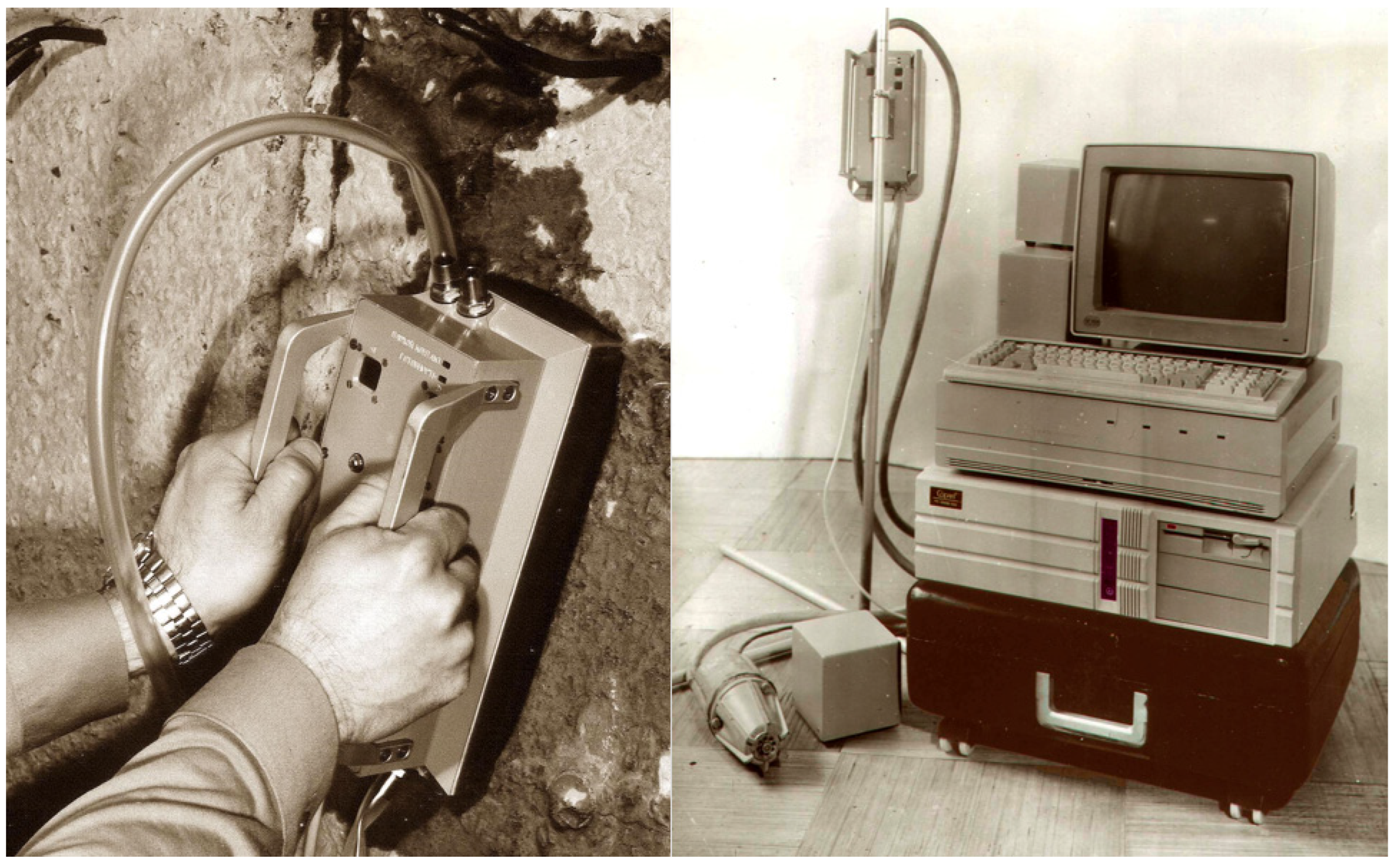
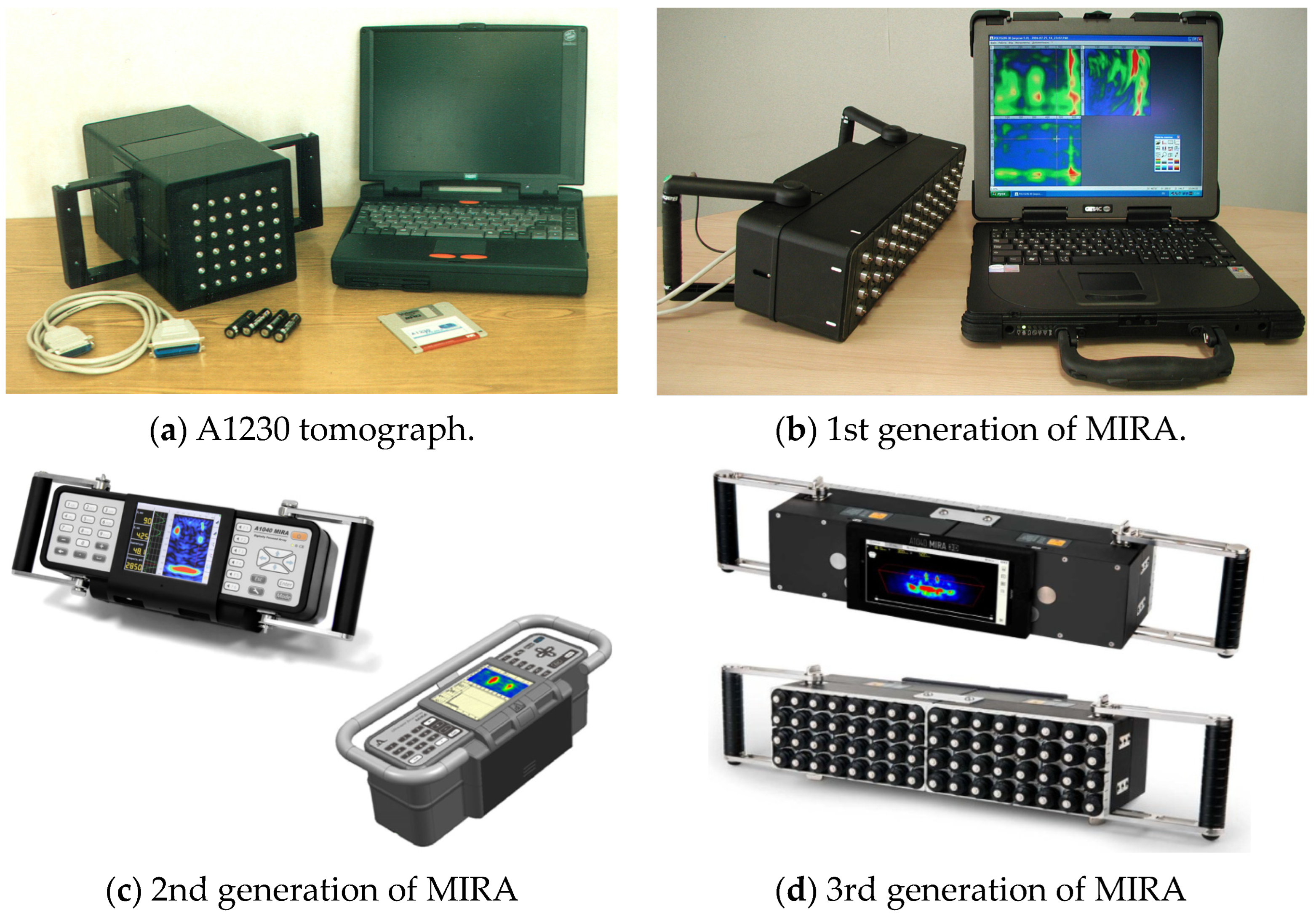
2. Historical Development of Ultrasonic Shear Wave Devices

In 1983, a division was created within the Research Institute of Introscopy (NIIIN) in Moscow, USSR with the mission to develop an ultrasonic flaw detector for concrete. It was expected by NIIIN that such a detector would be used to search for internal defects in concrete structures such as shear walls, concrete slabs, building foundations, and other concrete elements with only one-sided access. More specifically, the requirements for the future device were set including: (1) the ability to detect concrete cavities the size of a table tennis ball at a depth of up to 1 m, and (2) a resolution along the front and depth no worse than 10 cm. A literature search conducted by the research team indicated that such equipment/devices did not exist. For comparison, the impact echo (IE) method was only introduced in 1986 [3]. However, it should be noted that the IE method detects concrete thickness or flaws based on frequency analysis.

In 1985, the research team at NIIIN started making progress toward the future design of the equipment. After numerous experiments with solid damping materials and devices that match the impedances of piezoceramics, they came up with the idea to use a liquid paste-like material as a damper [4]. In terms of matching devices, they proposed using a rod with an impedance equal to the impedance of a piezoelectric element [5]. They completed the study of the attenuation coefficient of ultrasound in different concrete mixes, which suggested, for concrete inspection, the spectrum of the signals to be used should not go into the frequency range above 150 kHz [6]. However, even with such a frequency range, another issue was observed. Specifically, the entire time window of the obtained signals was occupied by slowly decaying structural noises that are caused by multiple reflections of waves from coarse aggregates [7].

In 1986, along with the study to improve the design of the transducers [8], the NIIIN research team directed its effort toward understanding the correlation between structural noises when moving transducers over a concrete surface. Specifically, experiments were conducted to find the minimum distance to move the receiving transducer so that structural noises from the subsequent scan will be uncorrelated with/unrelated to those from the initial position. The idea was that unrelated structural noises will not be accumulated when signals from an array of transducers are used for image reconstruction [9,10]. Instead, only related echoes from objects/defects of interest will be focused on, and therefore, visualized with the so-called synthetic aperture focusing technique (SAFT). Through the aforementioned experiments, the minimum distance was found to be between 15 and 20 mm for most concrete mixes.

In 1987, the research team designed and manufactured a multi-element 100 kHz ultrasonic transducer with an aperture of about two wavelengths. It consisted of a matrix of piezoelectric elements connected in phases and filled with a liquid damper. With this transducer, it made it possible to see the concrete backwall signals on the oscilloscope screen [7]. To a certain degree, even signals from spherical reflectors with diameters of 50 and 100 mm at a depth of almost 250 mm were visible. Refined studies of the correlation between structural noises on the concrete surface were carried out using transducers with different apertures. They confirmed the assumption that any ultrasonic transducer with an aperture smaller than the minimum distance mentioned above will not provide spatial signal accumulation against the background of structural noises [9,10].

After several transducer-array (tomograph) models were manufactured and tested in 1988, the NIIIN research team solved another important issue, testing on vertical surfaces. Specifically, when the tomographs were tested on vertical surfaces as shown in Figure 1, a liquid had to be used to maintain the acoustic contact between the transducers and the tested concrete. For that, water was pumped from a bucket to the antenna device through a hose. The pump was controlled by a computer, and the control information was given by the acoustic contact of all elements of the array with concrete. As a consequence, after a period of testing, the area was filled with a large amount of water.

To solve the above problem, the NIIIN research team started working on the creation of ultrasonic transducers with dry point contact (DPC). The first model of these transducers was developed so that metal balls with a diameter of about 2.5 mm were fixed with epoxy resin in the centers of their working surfaces. It was observed that the strength of received signals dropped very significantly, but the shape of the signals was preserved. With a pair of those transducers with DPC, the research team physically modeled several positions of the transducer array on the concrete surface. It was found that the obtained tomograms were not much inferior to those acquired earlier with liquid contact under the same other conditions. This result helped the research team to see the opportunity for creating and commercializing dry contact systems. Accordingly, an entity was established in 1991 and is known today as Acoustic Control Systems—ACS Group.

In 1992, the ACS Group developed a transducer array based on longitudinal waves (p-wave) with DPC and a transmitting-receiving device for it [11]. Since the strength of signals from that array was 40–50 dB lower than those from a transducer array with a liquid contact, they decided to place the excitation pulse generator and the preamplifier in the housing case. The protector (contact tip) of the transducers was made in the form of a metal cone with a height of about 4 mm. For all transducers of the array to stay attached to the tops of their protectors while on an uneven concrete surface, the body of the electroacoustic part of the array had a spring-loaded suspension. In addition, to eliminate the mutual interference of transducers in the array due to airborne acoustic coupling, an acoustic screen was installed on the body of each transducer.

The same year, the ACS Group worked on the development of an ultrasonic device for quality control of decorative plates used in the construction and renovation of buildings. While the control method was traditional, i.e., measuring the time or speed of the passage of an ultrasonic signal when sounding through the slab, it was unconventional in a way that the device had to work with both longitudinal and transverse/shear waves through dry contacts. The research team was able to find a solution by controlling the phases of two piezoelectric elements. Specifically, if the piezoelectric elements are switched on in phases, then the protector performs longitudinal oscillations and the transducer emits longitudinal waves. On the other hand, if the piezoelectric elements are turned on in the antiphase, then the transducers will emit and receive transverse waves [2,12,13,14].

In 1995, the first shear wave transducer array with DPC was manufactured and commercialized by the ACS Group as an A1230 tomograph. As shown in Figure 2a, it consisted of an antenna device and a personal computer [15]. The antenna device consisted of 36 transducers (6 × 6) arranged with a 20 mm step. Their operating frequency was 55 kHz. The width of the spectrum of ultrasonic signals at a level of minus 6 dB is about 100% of the operating frequency. The research team carried out a detailed study of the signal-to-noise ratio in concrete in which the ratio values were compared between the longitudinal and transverse waves. The result was that the signal-to-noise ratio for the shear wave was on average 10 dB higher than the one for the longitudinal wave. With that, the advantage of the transverse/shear wave over the longitudinal wave for echo tomography of concrete structures was finally comprehended [16]. For this reason, DPC shear wave transducers have become a standard component in most concrete imaging devices later manufactured by the ACS Group, of which MIRA has been the most advanced and well-known equipment. Since MIRA has been the ultrasonic shear wave device used in most of the studies found in the literature, the next section is dedicated to describing the main features of this equipment.

3. Description and Main Features of MIRA

The ACS Group manufactured the first generation of MIRA in 2007. As depicted in Figure 2b, the device consisted of 40 DPC shear wave transducers that were grouped into 10 blocks of four transducers. For the second generation shown in Figure 2c, the number of transducers was increased to 48, and accordingly, the number of blocks was 12. During operation, all four transducers within one block either transmit or listen to shear wave signals at the same time. The signals collected by each block of transducers are then averaged to produce a single A-scan. While the original purpose of such block design was to increase the signal-to-noise ratio for longitudinal objects that lie perpendicular to the device’s longitudinal axis, a problem with it is that small reflectors may not be visualized due to the averaging operation [1]. The third generation of MIRA (MIRA 3D and MIRA 3D Pro), shown in Figure 2d, with the true three-dimensional capability, which is explained later on, was designed to resolve the issue. In these devices, each transducer can transmit/receive shear wave signals independently. The number of transducers for MIRA and MIRA 3D Pro is 32 and 64, respectively.

Other than the number of transducers or block design, the three generations of MIRA are almost the same in other aspects. For example, all the transducers are based on DPC technology, and they are independently spring-loaded so that the device can be deployed on a relatively rough surface. The transducers can be operated with a center frequency in the range of 25 to 85 kHz. During the operation of the device, the laser light is provided to assist the operator in positioning the device correctly on marked survey locations. Ultrasonic shear wave data (A-scans) obtained from the transducers are processed onsite to show on the display screen the two-dimensional images (B-scans) of each scan location. For a complete survey performed on a perpendicular grid, i.e., using map mode, the data can be processed by proprietary software to generate a 3D image of the structure. Such 3D images can be further analyzed by looking at the C- and/or D-scans for any location [1,2].

It is necessary to understand how the device collects the data for each survey location. For the block design previously mentioned in the first and second generations of MIRA, each block of transducers is activated in succession, while the non-activated blocks/transducers behind it listen for the ultrasonic shear wave signals [1]. Since only one A-scan is generated for each pair of transducer blocks, the number of A-scans for each survey location will depend on the number of blocks in the system. That said, the number of A-scans generated for each location will be 45 ($\frac{10\times 9}{2}$) and 66 ($\frac{12\times 11}{2}$) for the first and second generations of MIRA, respectively. In the third generation, while block (linear mode) is still a setting option, the matrix mode, as the name suggests, allows each transducer to work independently as a transmitter or receiver. In this mode, since each transducer is also activated in succession while those behind it listen to shear wave signals, the number of A-scans obtained for each location is 496 ($\frac{32\times 31}{2}$) and 2016 ($\frac{64\times 63}{2}$) for MIRA 3D and MIRA 3D Pro, respectively.

For data processing, the MIRA employs the synthetic aperture focusing technique (SAFT)—an algorithm invented in the late 1960s for medical imaging applications [17]. Due to the ease of its implementation, the SAFT has been applied to many other areas [18,19,20,21,22], including nondestructive testing and evaluation of concrete structures [23,24,25,26,27,28,29,30,31,32]. For the first and second-generation MIRAs, only the 2D-SAFT can be applied to generate the cross-sectional image of the scan location because of the 2D nature of its data [32]. On the other hand, when the matrix mode is used with the device of the third generation, the 3D-SAFT will help generate the 3D/volumetric image of the survey area [32]. Detailed descriptions of the 2D- and 3D-SAFT were provided in [32], which can be applied to both ground penetrating radar (GPR) and MIRA data. For clarification, both technologies are based on the principles of wave propagation. The only difference is the physical nature of each wave type where the first uses electromagnetic waves and the second uses ultrasonic shear waves.

In addition, another characteristic of the device involves the so-called array polarization [1], and the directionality of the shear waves being transmitted and received by its transducers [2]. The former is caused by the block design of the device of the first and second generations. As illustrated in Figure 3, it leads to the fact that the device can see well the reflecting objects that lie in a direction parallel to the transducers in each block (due to the signal travel time being the same for all four transducers). Regarding the latter, the orientation of the reflecting object relative to the vibration direction of the transducer tip may influence the strength of the signals being recorded. As can be realized, a combined consequence of those two effects is that, in addition to the size of an entity/defect, the orientation of the device during data collection will affect its visibility/detectability in the final image.

4. Review of MIRA Applications

The following sections provide an overview of applications of ultrasonic testing using MIRA, including concrete thickness measurements, detection and characterization of delamination and cracks, detection of rebars, voids and honeycombing, and the assessment of grouting in post-tensioning ducts.

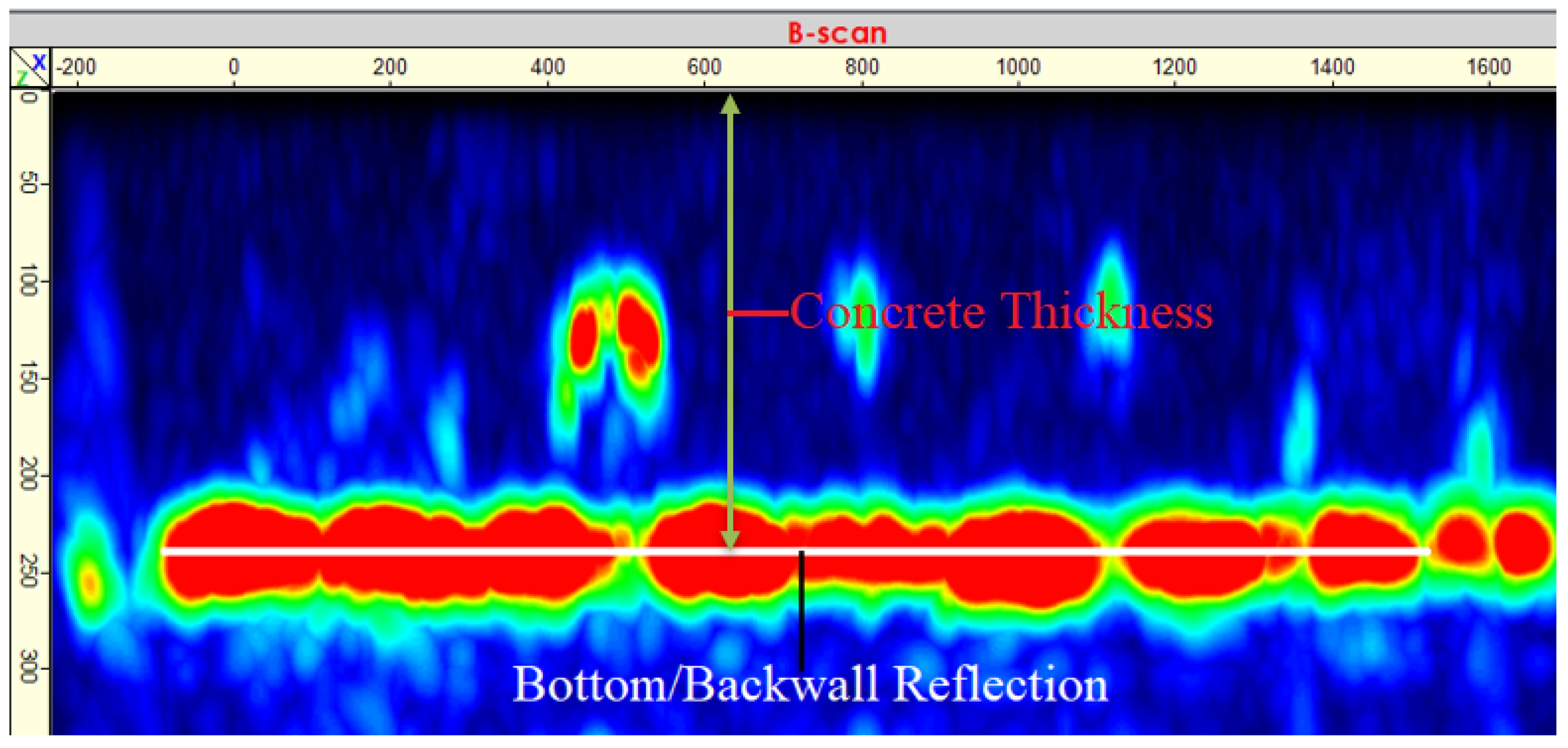
4.1. Concrete Thickness Measurement

According to the MIRA developers [33], measuring the thickness of concrete elements with one-sided access was among the first intended uses of ultrasonic shear wave devices. In the literature, this application has been studied primarily for concrete pavements [34,35] and concrete bridge decks [1]. For that, the thickness of concrete at a scan location was measured manually and directly from the B-scan image obtained with the proprietary software based on the SAFT algorithm. As illustrated in Figure 4, such a thickness value was measured from the top concrete surface to the location/point corresponding to the peak of the bottom/backwall reflection. For pavements, it was reported that the thickness obtained in this manner correlates well with the ground-truth information from concrete coring, with the R-squared values of 0.967 and 0.9968 for [34,35], respectively.

As for the bridge decks, it was reported in [1] that the maximum difference between the deck thickness measured by the device and those obtained with a fresh ruler was 24.9 mm. In terms of repeatability, while the average difference in thickness between two ultrasonic measurements for one location was about 18 mm, the maximum difference was reported to be up to 32 mm. The main reason behind this, as pointed out by [1], was the error associated with the shear wave velocity measurement. Although one may certainly refer to the above values when accounting for thickness errors, more comprehensive studies are still needed by the construction industry to make ultrasonic shear waves a standardized technique for concrete thickness evaluation. In such studies, a standard data collection/processing procedure should be developed, along with a full assessment of factors that may affect thickness measuring results.

4.2. Rebar Detection and Evaluation

The most noticeable application of MIRA has been to locate and visualize rebars within concrete [1,2]. Concerning the detailed characteristics of rebars, the device has been reportedly used to detect cover thickness (rebar depth), rebar diameter, and the bonding quality of rebar/concrete.

For the first item in that list, it was found by [34] that the device could determine the concrete cover with an accuracy significantly greater than the magnetic-based pachometer/rebar locator/cover meter results. Specifically, when correlated with rebar depth measured from concrete cores for two different datasets, the depth values obtained with MIRA yield a much higher correlation coefficient than those taken from pachometer measurements (R² of 0.991 for MIRA vs. R² of 0.186 for pachometer). However, the authors of the above study also acknowledged that more data would be needed for a statistically sound validation given the fact that only seven cores were used in their research.

Related to both cover thickness and rebar size characteristics, two-dimensional full waveform inversion (2D FWI) was used in a very recent study [36] to determine both the depth and diameter of rebars from ultrasonic shear wave data. Concerning the former, it was reported that, for twenty rebars of varying size and/or depth, the cover thickness can be reliably predicted with an error of less than 12%. In terms of the size, of those twenty rebars, the method was able to predict the diameter of 95% rebars (19/20) with less than 33% error, or 80% rebars (16/20) with less than 26% error. In a separate study [37] when the same 2D FWI methodology was employed, an ultrasonic shear wave device clearly showed its capability to visualize and detect steel bar/concrete debonding, the last item in the aforementioned list.

4.3. Concrete Delamination

Delamination is a common type of concrete defect, which manifests as a separation, splitting, or cracking of concrete along a plane parallel to a surface. As summarized by [38], the common causes of delamination include (a) the use of air entrainment in a concrete slab receiving a hand trowel finish; (b) machine-trowel finishing a lightweight aggregate concrete slab; (c) premature finishing of a slab before the cessation of bleeding; (d) top-down stiffening or surface crusting of a concrete slab under hot, windy, or dry weather conditions, especially if the slab is undergoing slow and prolonged bleeding; (e) prolonged finishing operations on an outdoor air-entrained concrete slab or on a slab receiving a mineral or metallic surface hardener; (f) corrosion of reinforcing steel in concrete due to chloride ingress or carbonation; and (g) cyclic freezing and thawing of a poorly or non-air-entrained concrete slab at critically saturated conditions. Regardless of its underlying cause, delaminations reduce the integrity/load-bearing capacity and accelerate the deterioration of concrete structures. Therefore, early detection of it is necessary [27,37,39].

Early results in [27,34,39] indicated that MIRA could directly detect deep delaminations and provided an indication of the presence of shallow delaminations that are at depths smaller than 65 mm. However, in [37,40], it was shown that images obtained using full-waveform inversion (FWI) of ultrasonic shear wave data clearly showed shallow (65 mm), intermediate (80 mm), and deep (130 mm) delaminations. Concerning the detectable size of delamination, it was reported in [1] that the device failed to identify 100 × 100 mm delamination regardless of its depth. The study also mentioned interpolation artifacts when non-square defects appeared to be rectangular in the obtained 3D images. Other than those issues, the successful use of the device for characterizing concrete delamination was also reported in other studies such as [30,41].

4.4. Concrete Voids and Honeycombs

Assessing the quality of concrete consolidation is among the most common applications of nondestructive evaluation (NDE) technologies in the construction industry. According to [42], such quality problems may arise due to the movement of rebar after the initial set, over/under vibration, mix segregation, and the development of bleed water pockets. Their common consequence is that voids are entrapped within a concrete element and compromise its structural integrity. Since ultrasonic wave energy encounters a nearly perfect reflection at the concrete/air interface, ultrasonic shear wave devices are supposed to be an excellent tool to detect voids and honeycombs in concrete.

That said, it has been shown that while ultrasonic devices can directly visualize large voids in concrete, they cannot do the same for honeycombs, which are concrete consisting of multiple close voids. Specifically, it was found in [1] that, without the rebar masking effect, a void of significant size would appear clearly in the reconstructed images. On the other hand, it was reported in [42] that concrete honeycombs could only be detected indirectly by analyzing the relative strength of the backwall reflection. As can be imagined, multiple voids within poorly consolidated concrete will refract ultrasonic waves and less energy will be able to reach the backwall of the structure before coming back to the concrete surface.

4.5. Grouting Condition of Embedded Ducts

Embedded post-tensioning tendons are commonly used in the construction of long-span bridges, elevated structures, residential foundations, walls, and columns. As to their design, each tendon is housed within a duct, which can either be metal or plastic. The ducts are then filled with grout, which is usually cementitious material so that the tendons can effectively redistribute stress within the structure and are protected from corrosive agents. Grouting defects, such as voids in post-tensioning ducts, will likely compromise structural integrity and reduce structural durability. Since severe tendon deterioration and failures have taken place in the past due to the presence of air voids within the duct [43], there is a growing need for technologies capable of finding those defects.

Accordingly, ultrasonic shear wave tomography has been on the list of candidate technologies to address the aforementioned problem. However, it has been reported that, other than the capability to detect the location of tendons, ultrasonic shear wave devices were unable to identify grouting defects. To be specific, it was reported in [1] that, for both plastic and metal ducts, while localization of the ducts was possible in the B-scan images, the shape and reflection patterns were not consistent enough to determine the grouting condition within them. That same conclusion was reached in a separate study [43] when ultrasonic shear wave tomography was compared with GPR, impact echo, and ultrasonic echo on their ability to identify grouting defects.

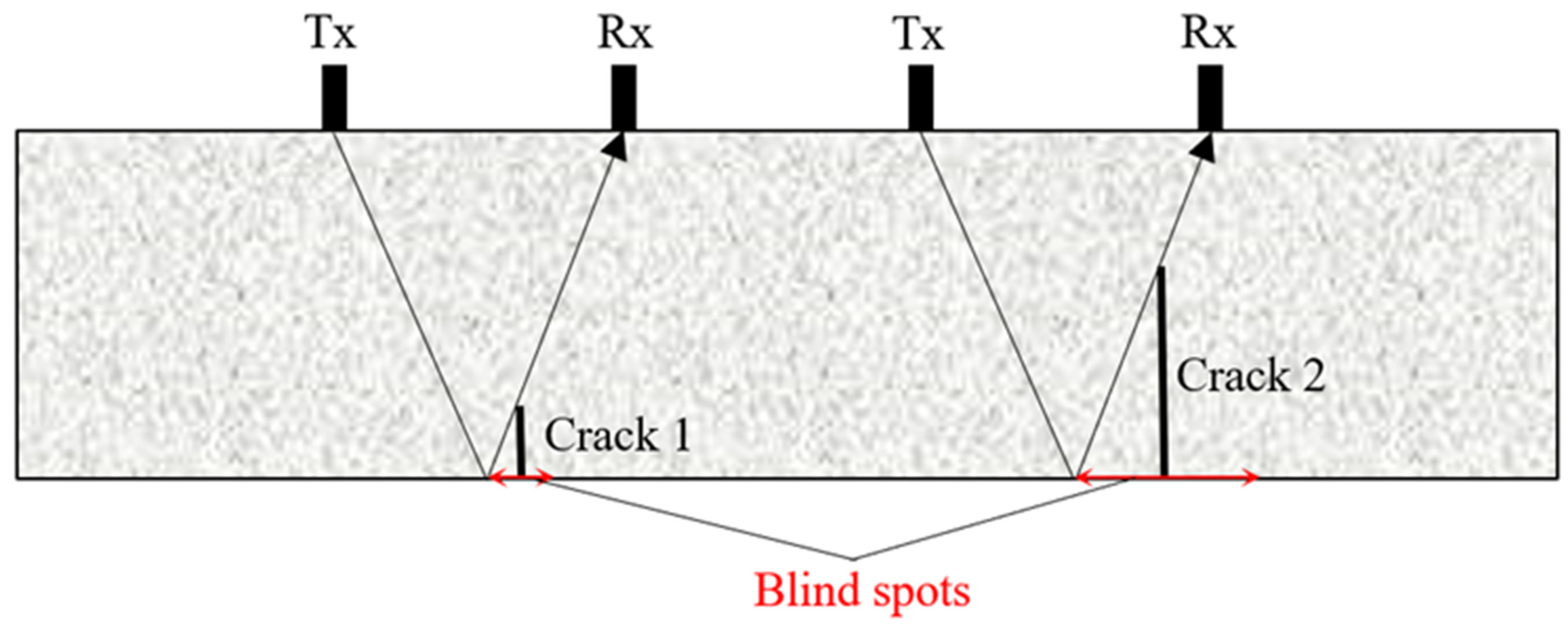
4.6. Characterization of Visible Cracks

Surface/opening cracks are common defects in concrete that lead to rapid deterioration and early failure of structures [44]. Specifically, those cracks provide the shortest path for corrosive agents such as oxygen, water, and chloride to reach steel reinforcements that will over time initiate rebar corrosion and accelerate element deterioration. Thus, this type of defect must be detected and characterized, most importantly the depth of a crack, to take appropriate maintenance actions.

That being said, several efforts have been made to identify and/or characterize opening cracks with ultrasonic shear wave devices. In earlier research [42], when MIRA was used to survey an area of a concrete slab having open cracks on the other side of the scanning surface, the following was reported. At the location of the crack, there was a slight discontinuity in the backwall reflection, and that shadowing effect might be used as an indication of the presence of a crack. In later research [1], the device was used to study the visibility of open cracks on B-scan images subjected to a variation in crack depth. In terms of positioning, the device was placed on the same surface of an open crack at two typical locations: (1) right on top of the crack and (2) offset a certain distance from the crack. It was reported that the tip of the crack appeared clearly in all B-scan images obtained with the offset configuration and that was not the case with the images obtained when MIRA was centered right above the crack. However, it was also reported that the crack tip became invisible when B-scans were combined into a volumetric image. Finally, a recent study [45] reported that the crack depth could be estimated based on the time-of-flight of ultrasonic shear waves, the spacing between the transducers, and the wave speed.

5. Laboratory Experiments

This section describes imaging results from ultrasonic shear wave data collected by the MIRA 3D device on several concrete slab specimens. The primary objective was to understand and evaluate the capability of the device on solving some concrete imaging problems that have been discussed in the previous section. Since the main focus is placed on a thorough understanding of the ability and accuracy of the data obtained with the system, the images presented hereafter were generated using the program developed in this study based on the 3D-SAFT algorithm, which consists of four main steps as described briefly in the following section.

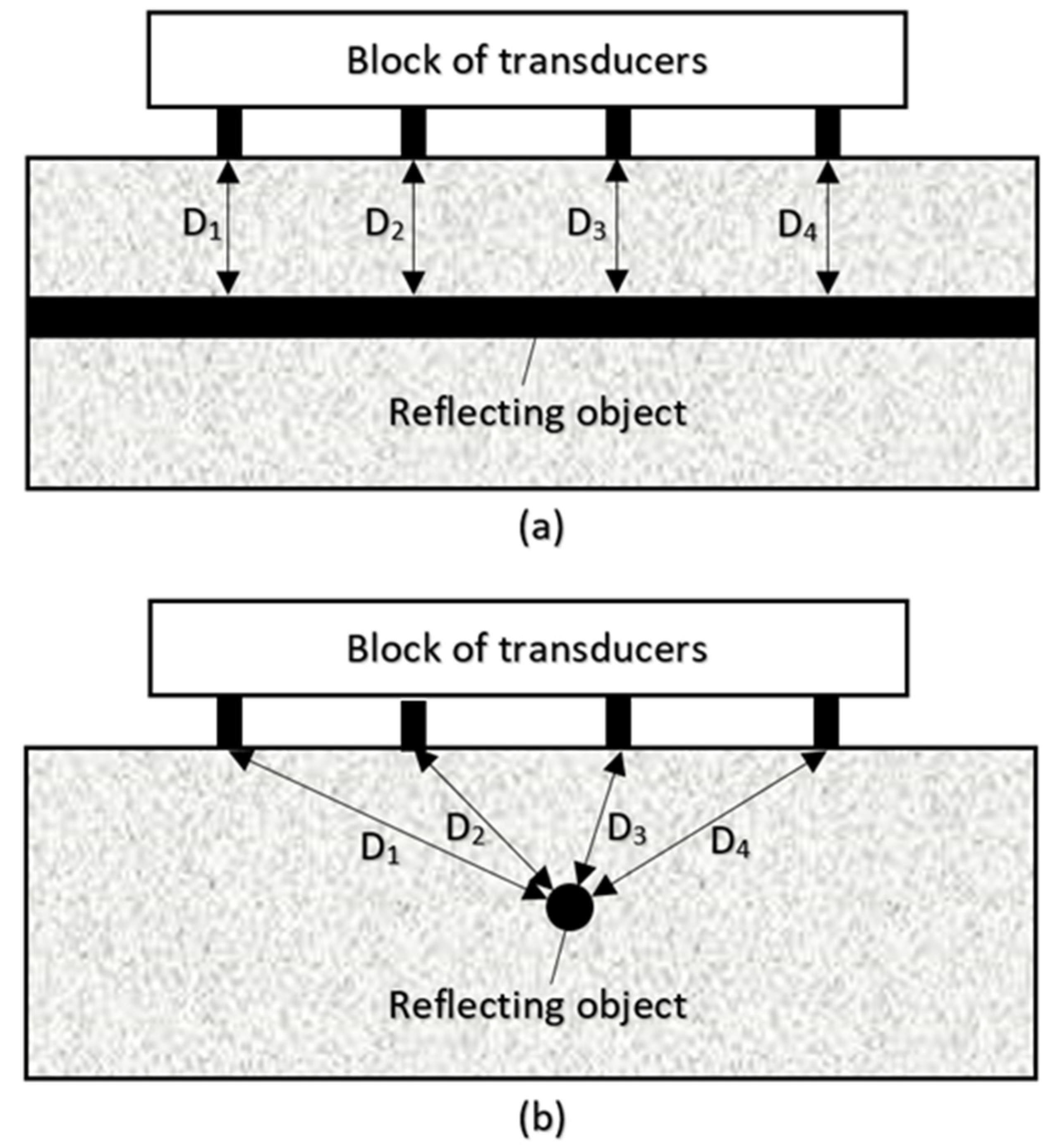
5.1. 3D-SAFT Algorithm

5.1.1. Determine Region of Interest

The region of interest is the area below the test surface where one would like to display the imaging result. For the 3D-SAFT algorithm, this region is the 3D space/volume right below the test area. Once this region is specified, its dimensions are sampled into small-size elements to form image points, the so-called voxels.

5.1.2. Compute the Sound Path Length for Each Image Point

Given the locations of transmitting (T) and receiving (R) transducers for each A-scan signal, this step identifies travel length of ultrasonic waves for each point in the imaged region. Specifically, given the coordinates of the transmitter (${\mathrm{x}}_{\mathrm{T}}$,${\mathrm{y}}_{\mathrm{T}}$,${\mathrm{z}}_{\mathrm{T}}$) and the receiver (${\mathrm{x}}_{\mathrm{R}}$,${\mathrm{y}}_{\mathrm{R}}$, ${\mathrm{z}}_{\mathrm{R}}$) corresponding to the i^th A-scan, the sound path length for an image point P (${\mathrm{x}}_{\mathrm{P}}$,${\mathrm{y}}_{\mathrm{P}}$,${\mathrm{z}}_{\mathrm{P}}$) can be calculated using Equation (1).

$${\mathrm{L}}_{\mathrm{P}}^{\mathrm{i}}=\sqrt{{\left({\mathrm{x}}_{\mathrm{P}}-{\mathrm{x}}_{\mathrm{T}}^{\mathrm{i}}\right)}^2+{\left({\mathrm{y}}_{\mathrm{P}}-{\mathrm{y}}_{\mathrm{T}}^{\mathrm{i}}\right)}^2+{\left({\mathrm{z}}_{\mathrm{P}}-{\mathrm{z}}_{\mathrm{T}}^{\mathrm{i}}\right)}^2}+\sqrt{{\left({\mathrm{x}}_{\mathrm{P}}-{\mathrm{x}}_{\mathrm{R}}^{\mathrm{i}}\right)}^2+{\left({\mathrm{y}}_{\mathrm{P}}-{\mathrm{y}}_{\mathrm{R}}^{\mathrm{i}}\right)}^2+{\left({\mathrm{z}}_{\mathrm{P}}-{\mathrm{z}}_{\mathrm{R}}^{\mathrm{i}}\right)}^2}$$

(1)

5.1.3. Assign Intensity Value for Each Image Point

In this step, each image point is assigned an intensity value based on the sound path length (${\mathrm{L}}_{\mathrm{P}}^{\mathrm{i}}$) calculated in the previous step. Specifically, given the signal velocity (V), that length is used in Equation (2) to compute the signal travel time corresponding to each image point (${\mathrm{T}}_{\mathrm{P}}^{\mathrm{i}}$). In turn, the obtained travel time is used in Equation (3) to find the intensity value that will be assigned to the image point (${\mathrm{I}}_{\mathrm{P}}^{\mathrm{i}}$). For each A-scan, this step is completed when all the image points have been assigned an intensity value. It is important to note that, to maintain the phase information, raw A-scans were used in this study without any transformation.

$${\mathrm{T}}_{\mathrm{P}}^{\mathrm{i}}=\frac{{\mathrm{L}}_{\mathrm{P}}^{\mathrm{i}}}{\mathrm{V}}$$

(2)

$${\mathrm{I}}_{\mathrm{P}}^{\mathrm{i}}={\mathrm{Ascan}}^{\mathrm{i}}\left({\mathrm{T}}_{\mathrm{P}}^{\mathrm{i}}\right)$$

(3)

where: ${\mathrm{Ascan}}^{\mathrm{i}}\left(\mathrm{t}\right)=$ The i^th A-scan signal.

5.1.4. Superposition of Images Obtained from All A-Scans

The unfocused images obtained from the previous steps are superposed to create the final image that shows reflective boundaries/surfaces. As expressed in Equation (4), the superposition is done for each image point by summing up the intensity values obtained from all A-scans in the synthetic aperture.

$${\mathrm{I}}_{\mathrm{P}}={{\displaystyle \sum }}_{\mathrm{i}=1}^{\mathrm{N}}{\mathrm{I}}_{\mathrm{P}}^{\mathrm{i}}$$

(4)

where:

• ${\mathrm{I}}_{\mathrm{P}}$ = Aggregated intensity value for image point P
• N = the number of A-scans in the aperture.

5.2. Experimental Results and Discussion

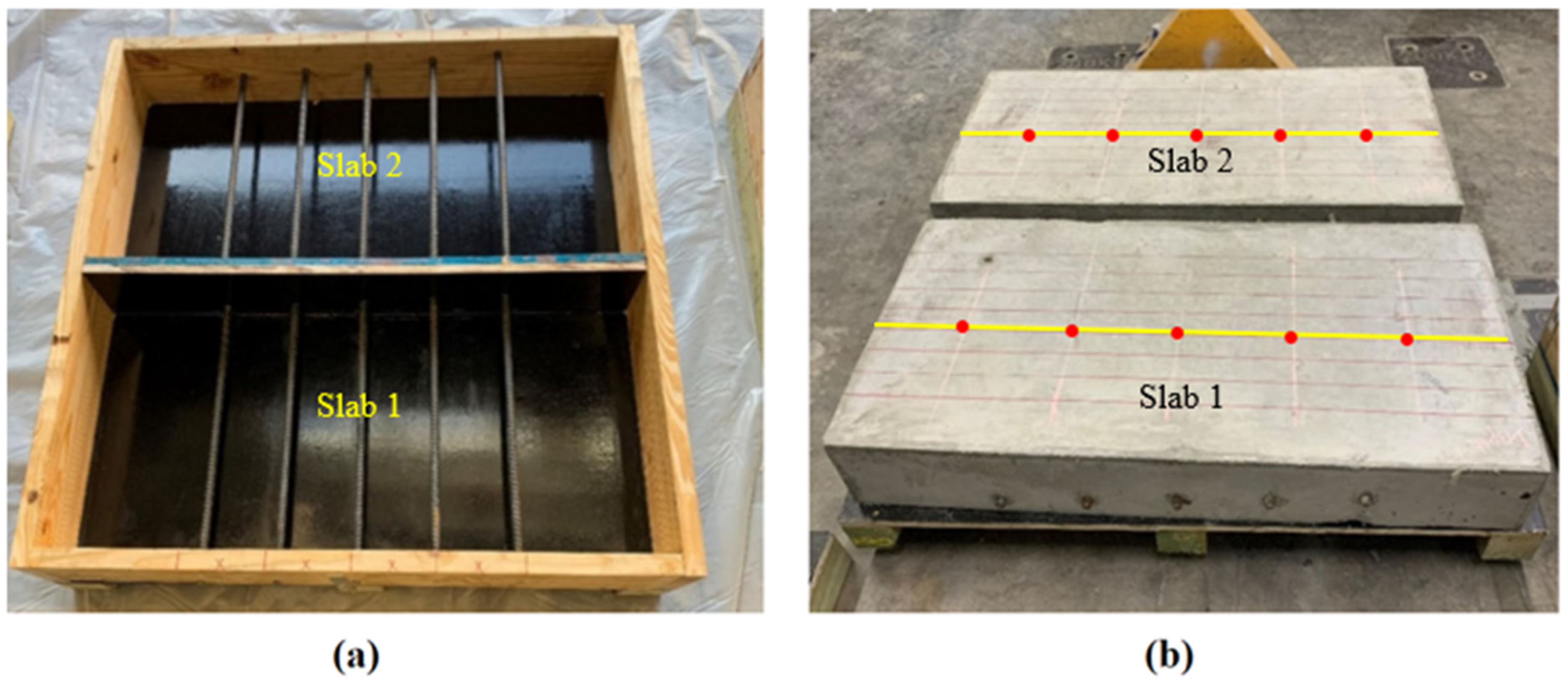
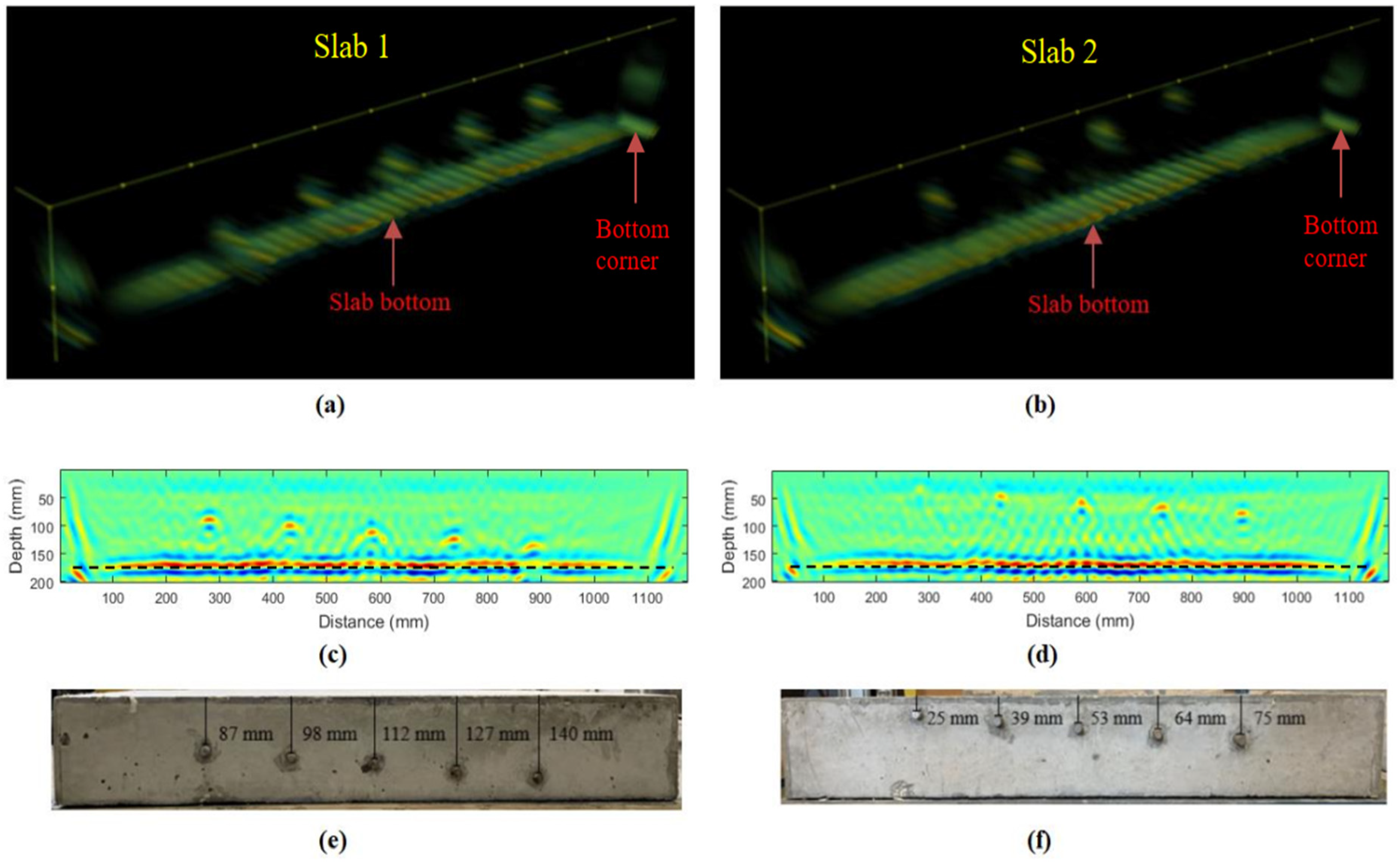
5.2.1. Slabs with Rebars of Varying Depth

This first experiment was conducted for two concrete specimens shown in Figure 5 (slab 1 and slab 2) with rebars of various depths ranging from 25 mm to 140 mm. The two slabs have the same dimensions of 1143 × 552 × 178 mm and were fabricated at the structural engineering laboratory on the main campus of the University of Florida in Gainesville, Florida (USA). Data was collected for each slab using MIRA 3D Pro shown in Figure 2d along the yellow lines in Figure 5b. As can be seen, each line consists of five red dots, each of which corresponds to the center of the device for each scan location. The distance between those red dots is 200 mm which is smaller than 375 mm, the longitudinal aperture of the device. Furthermore, the data was collected using the true 3D/matrix mode. Therefore, a volumetric image can still be obtained even with only one scan line. For clarification, it is noted that one would not be able to use interpolation with only one B-scan image.

The purpose of this test was to verify the capability of MIRA in measuring the rebar depth and the thickness of the concrete member. While the change of rebar depth can be observed from the 3D images in Figure 6a,b, specific values for slab 1 and slab 2 can be measured from the B-scans in Figure 6c,d, respectively. Those values can then be compared with the ground-truth values shown in Figure 6e,f. Concerning the thickness of the specimen, it can be determined for each slab by measuring the depth of each dashed black line in Figure 6c,d, which represented the peak of the wavelet from the backwall reflection. As can be verified, in all instances, the depth/thickness error is less than 1 cm.

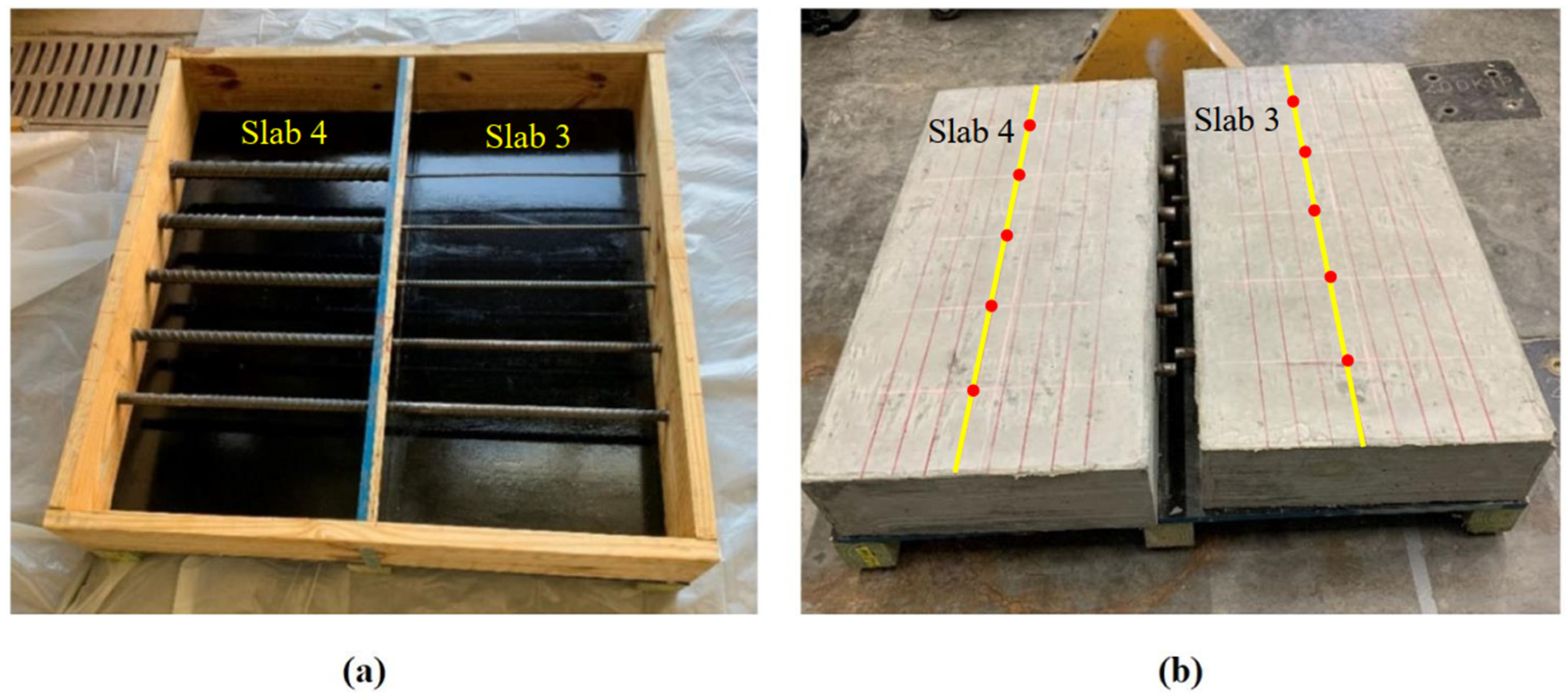
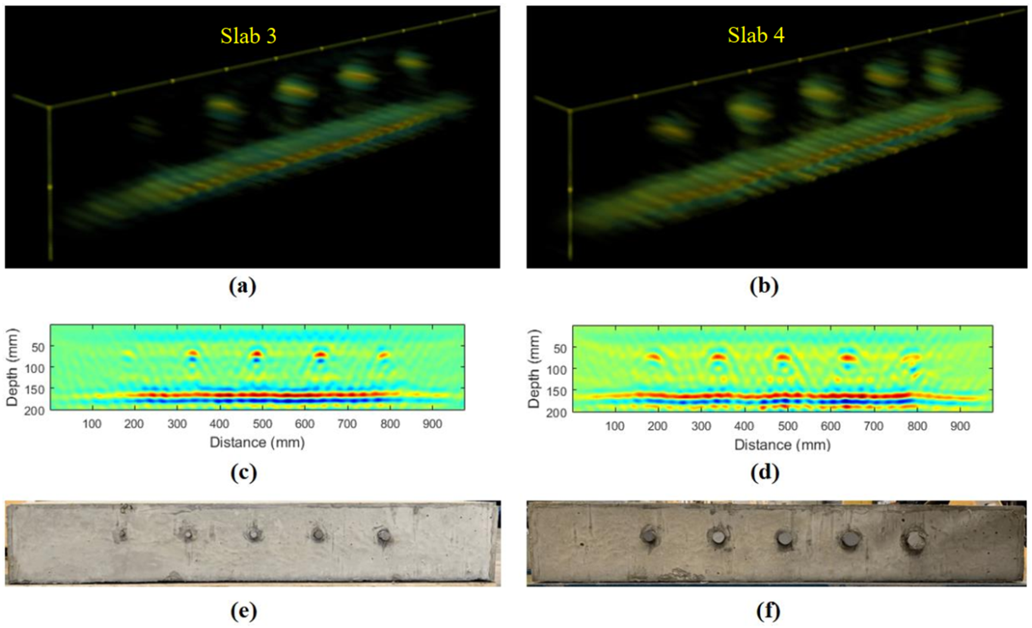
5.2.2. Slabs with Rebars of Varying Size

The objective of the test described in this section was to understand whether MIRA could be used to measure the rebar diameter with the conventional SAFT algorithm. For clarification, in the literature, rebar sizes were determined from the data but through the full waveform inversion (FWI) technique [36]. While FWI is powerful, a big limitation of it is that it is computationally demanding, which is not yet suitable for industry application. Two specimens (slab 3 and slab 4) of the same dimensions as the previous two slabs were cast and used in this experiment. As can be seen in Figure 7, they contain ten rebars of various sizes (#3, #4, #5, #6, #7, #8, #9, #10, #11, #14 in the US naming system). For each slab, the data were collected at five spots (red dots) along each yellow line in Figure 7b using MIRA 3D Pro. Like the previous experiment, the long axis of the device was oriented parallel to the scan line so that the cross-section of rebars would likely appear in B-scan images.

In line with the previous experiment and reported literature, the results in Figure 8 show that the device was able to visualize all rebars within the two slabs regardless of their diameter. In addition, while one can easily notice the effect of bar size on the image area surrounding each rebar location, it is very difficult to establish a clear criterion for predicting rebar diameter directly from SAFT-based B-scan images. This will be a topic of future study where image processing and machine learning techniques are used on B-scans to visualize and/or predict the rebar diameter. Furthermore, it should be noted that the density of A-scan signals has an important effect on the obtained images. That is another reason why the rebar on the leftmost side of Figure 9c does not appear as clearly as the others, in addition to the rebar size effect.

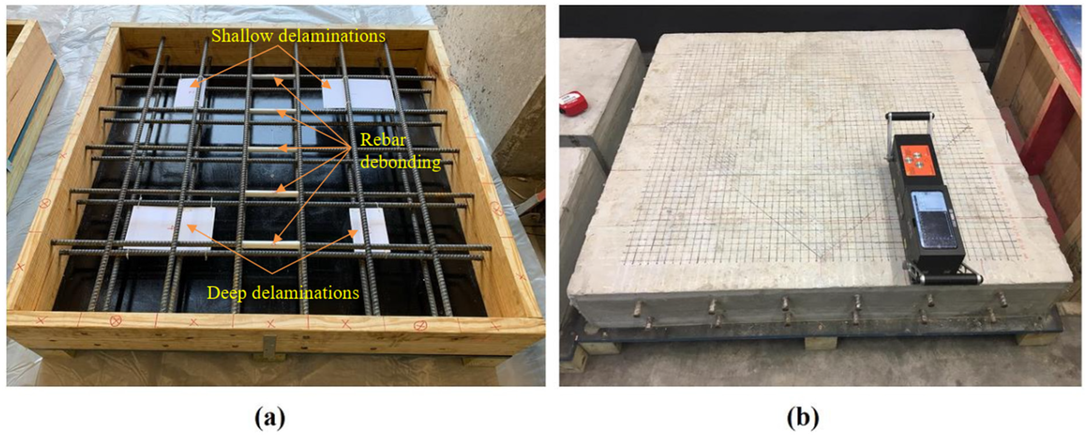
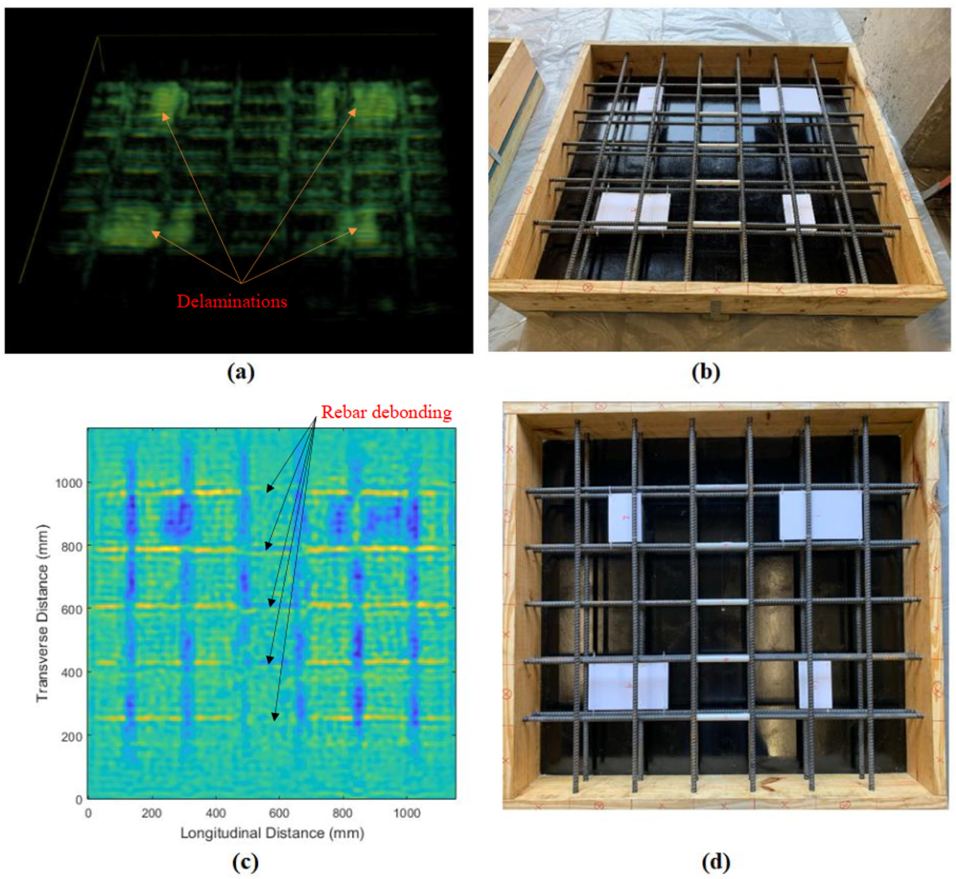
5.2.3. Slab with Rebar Debonding and Concrete Delamination

As shown in Figure 9, the specimen (slab 5) described in this section has a typical slab design with two layers of steel reinforcement. Each layer consists of 16 mm diameter rebars laid in both longitudinal and transverse directions. The slab has the dimensions of 1219 × 1219 × 178 mm and included two types of defects discussed in the literature section, namely steel bar debonding and concrete delamination. Steel bar debonding was created for five segments in the middle of the slab using a plastic wrap of increasing thickness (from 0.8 mm to 4 mm). Delaminations were made by foam embedded within the slab before pouring concrete. Four of them were different from one another either in size (102 × 152 mm and 152 × 254 mm) or depth (64 mm and 140 mm). MIRA 3D Pro was employed to scan from the top surface of the slab using the 3D/matrix mode. Since one objective of this experiment was to visualize the rebar debonding defect, the long axis of the device was oriented perpendicular to the segments of debonding rebars. The spacing between scan points was 200 mm in the scanning direction and 40 mm in the perpendicular direction.

Figure 10 presents the imaging results (Figure 10a,c) along with the photos of the specimen (Figure 10b,d) for comparison. As can be seen, the 3D image in Figure 10c clearly shows all the delaminations regardless of their size and depth. It is noted that, for clear visualization of rebar and delaminations, the image was filtered to not include the bottom/backwall reflections. The reflections from delaminations appear to be much stronger than those from rebars, which makes rebars less visible. That is reasonable because ultrasonic wave energy experiences a nearly complete reflection at the concrete/air interface.

Concerning steel bar debonding, a close look at the 3D image above clearly revealed the difference between debonded and bonded bar segments. However, since it is difficult to show such a difference in the 3D image in the presence of delamination and the bottom reinforcement layer, the C-scan shown in Figure 10c was selected for that demonstration. To be specific, that C-scan slices through the top layer of rebar, which contains the debonding segments. That being said, one can easily recognize the discontinuity of rebar images at the debonding locations. Theoretically, this is explained by the well-known effect of phase reversal, which is a phenomenon of both electromagnetic and ultrasonic waves. As a further note, also related to reinforcement, one might realize a great advantage of MIRA 3D in its capability to visualize all rebar objects from a survey in a single direction. For clarification, to obtain the same with the first and second generations of MIRA, one would have to survey an area twice by switching device orientation in between.

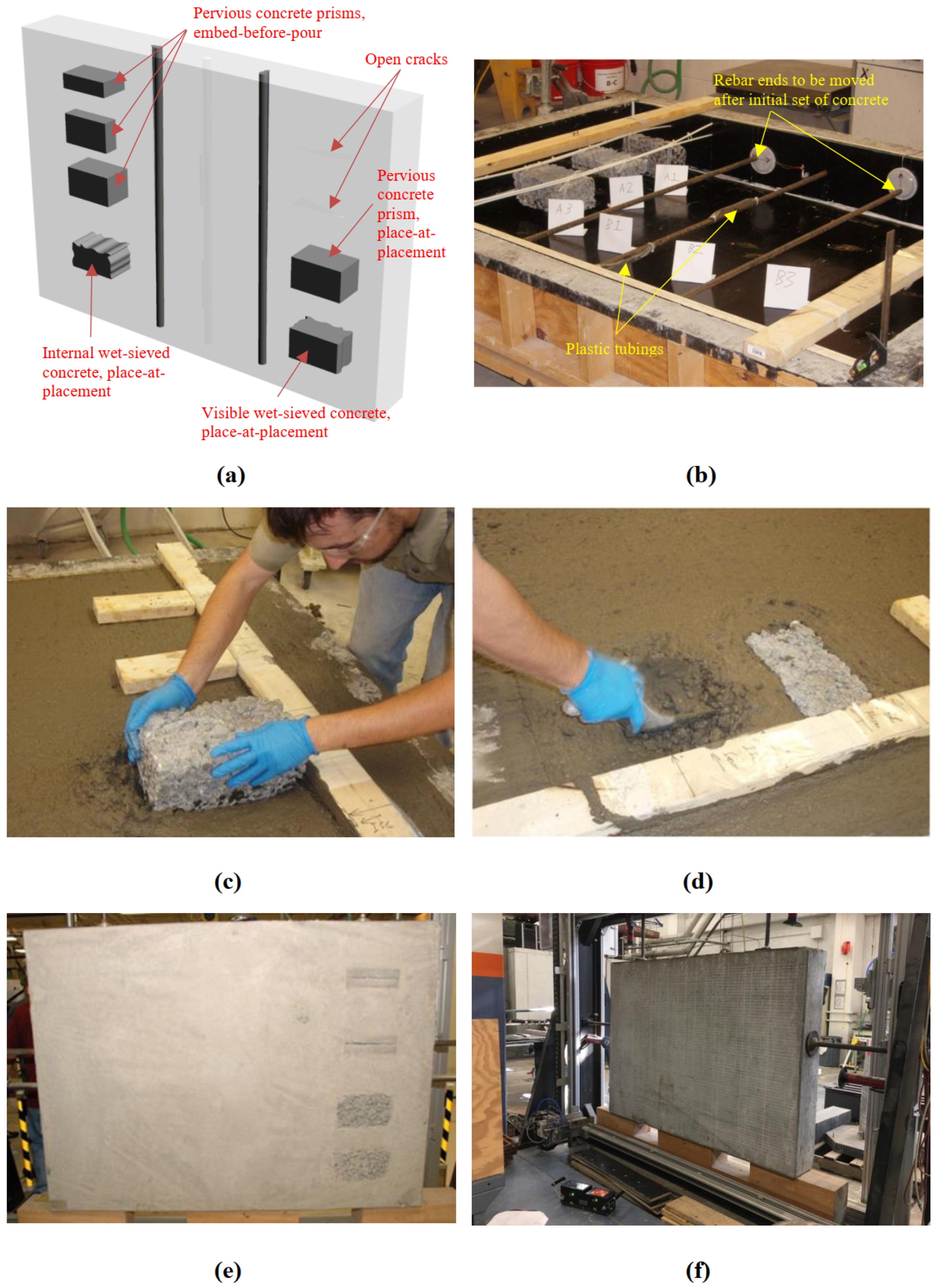
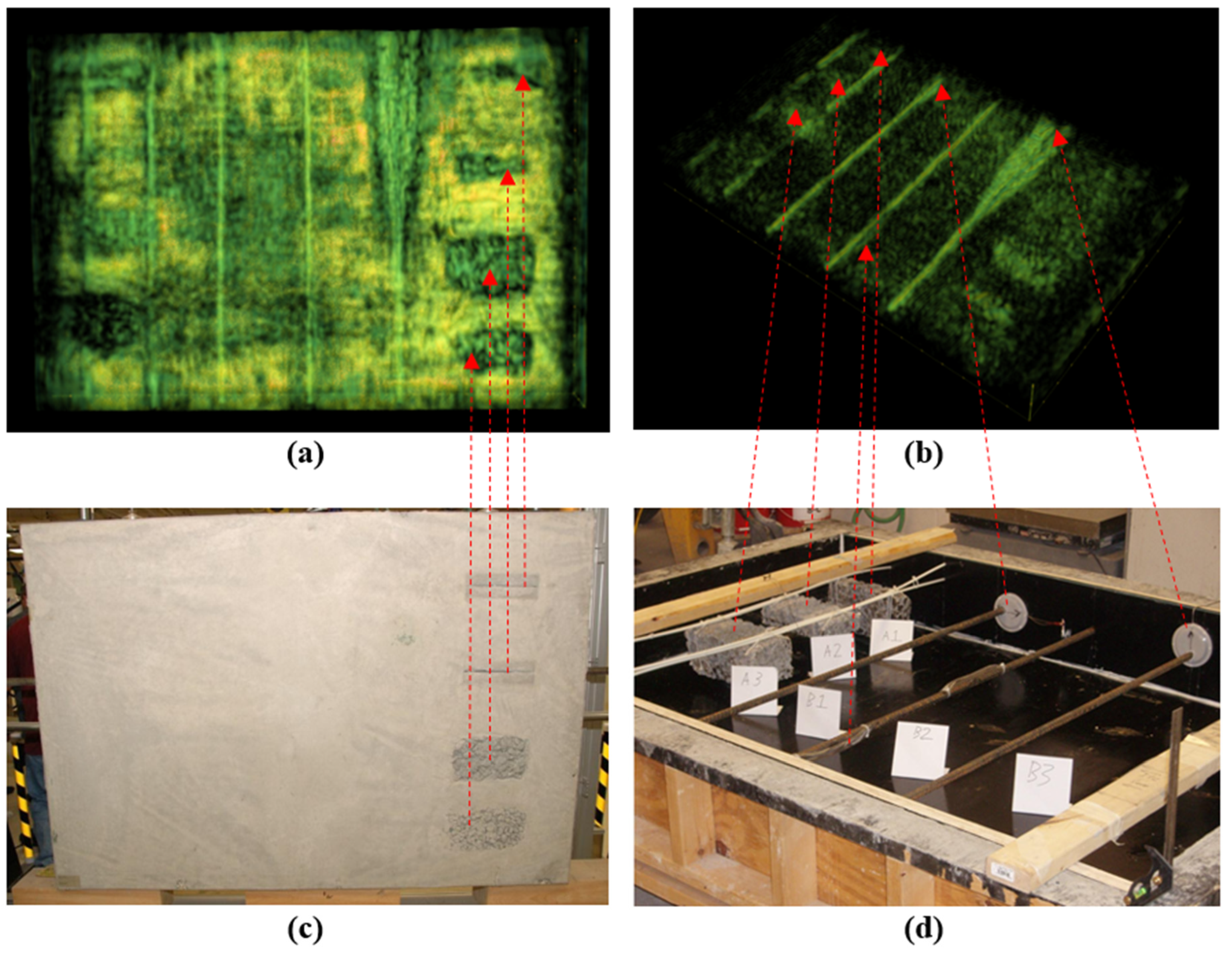
5.2.4. Slab with Voids, Honeycombs, and Cracks

The slab described in this section belongs to the Florida Department of Transportation’s (FDOT’s) NDE Validation Facility in Gainesville, Florida. As shown in Figure 11, it is an unreinforced concrete specimen with simulated cracking and non-consolidation flaws (i.e., voids/honeycombs). The slab is 1980 mm long, 1524 mm wide, and 254 mm deep. It contains three pieces of #6 rebar, one with two plastic tubings of different orientations attached to simulate entrapped air. The three rebars were embedded in the middle length of the slab, while simulated honeycombs and cracks were placed on both ends. Specifically, on one end area, three prisms of pervious concrete, i.e., simulated honeycombing, were suspended by two groups of small fiberglass rods along the central plane of the slab. The other end has one more prism placed at the surface level during concrete placement along with two triangular plates to simulate vertical cracks of varying depth. In addition, to create a more natural honeycombing on each end, at the time of concrete placement, a measure of the concrete mix wet-sieved to approximately the same volume as the embedded prisms were placed into the slab. A similar procedure was used on the end with the open cracks. Finally, as indicated in Figure 11b, an additional type of defect was created by moving one end of the rebar after the initial set of concrete. In doing so, it was expected that an increasingly severe trail of disturbed concrete behind the path of the rebar would be created. However, it was reported that the laterally moving rebar (the left one in Figure 11b) only moved 8 mm, which was much smaller than 25 mm, the expected value for both rebars [42].

It should be noted that the above slab has been scanned before with the previous version of MIRA and the details of such scans can be found in [42]. Therefore, in the following, some of those details will be discussed along with the survey in this study, which employed the latest version of the device (MIRA 3D). Starting with data collection, the present study also surveyed the slab from the surface without visible defects. However, while in the previous study the slab was scanned in two perpendicular directions, for the time being, in this study it was surveyed horizontally only, as demonstrated by the marked grid in Figure 11f. The imaging results are described and discussed in the subsequent paragraphs.

For the convenience of comparison, the imaging results are presented in Figure 12 alongside the photos of the slab that indicate the ground-truth condition. The 3D views in Figure 12a,b were oriented to closely replicate the view of the slab in corresponding pictures (Figure 12c,d). In all images, the slab is viewed from the side that has visible defects, which is the bottom/backwall from a data collection viewpoint. In addition, for a clear view of the internal elements and defects, the backwall reflections have been removed before rendering the 3D view in Figure 12b.

Most voids can be seen clearly in the 3D images. Those include the voids from the plastic tubings, and the voids created by moving one rebar end after the initial set of concrete. Concerning the former, while a close look at the 3D image revealed the effects of both tubings, the one attached horizontally to the rebar appeared more visible than the other, which was masked by the rebar on top. For the latter, one can easily see a region of expanded volume at one end of a rebar, which corresponds to the void caused by moving it vertically after the initial set of concrete. The same effect is less visible for the lateral moving rebar since, as previously mentioned, it only moved a distance of 8 mm.

Concerning honeycombing, interesting results were obtained where both types of simulated honeycomb, namely pervious concrete prisms and wet-sieved concrete, appeared very clearly in the 3D images. As can be seen, they are manifested via the following two effects. First, there is a significant drop in the backwall reflection strength below a honeycombing area because less energy can reach the slab bottom. Second, small voids within a honeycomb can be seen directly in the 3D images. While the first effect was already reported in the literature for the same slab specimen [42], the second effect is a new observation of this study, which was enabled by the 3D capability of the device.

Concerning the two open cracks, while the crack tips cannot be seen clearly within the 3D volume, the crack depth has a noticeable effect on the backwall visualization. Specifically, as can be observed in Figure 12a, there appear to be two isosceles triangles whose height corresponds to the surface location and whose bottom matches the deepest end of each crack. In other words, it appears that when the crack depth increases, it tends to create a wider shadow area in the backwall reflection. This is fully understandable considering how a crack intercepts the ultrasound ray path of the bottom reflection. A schematic explanation of this is provided in Figure 13.

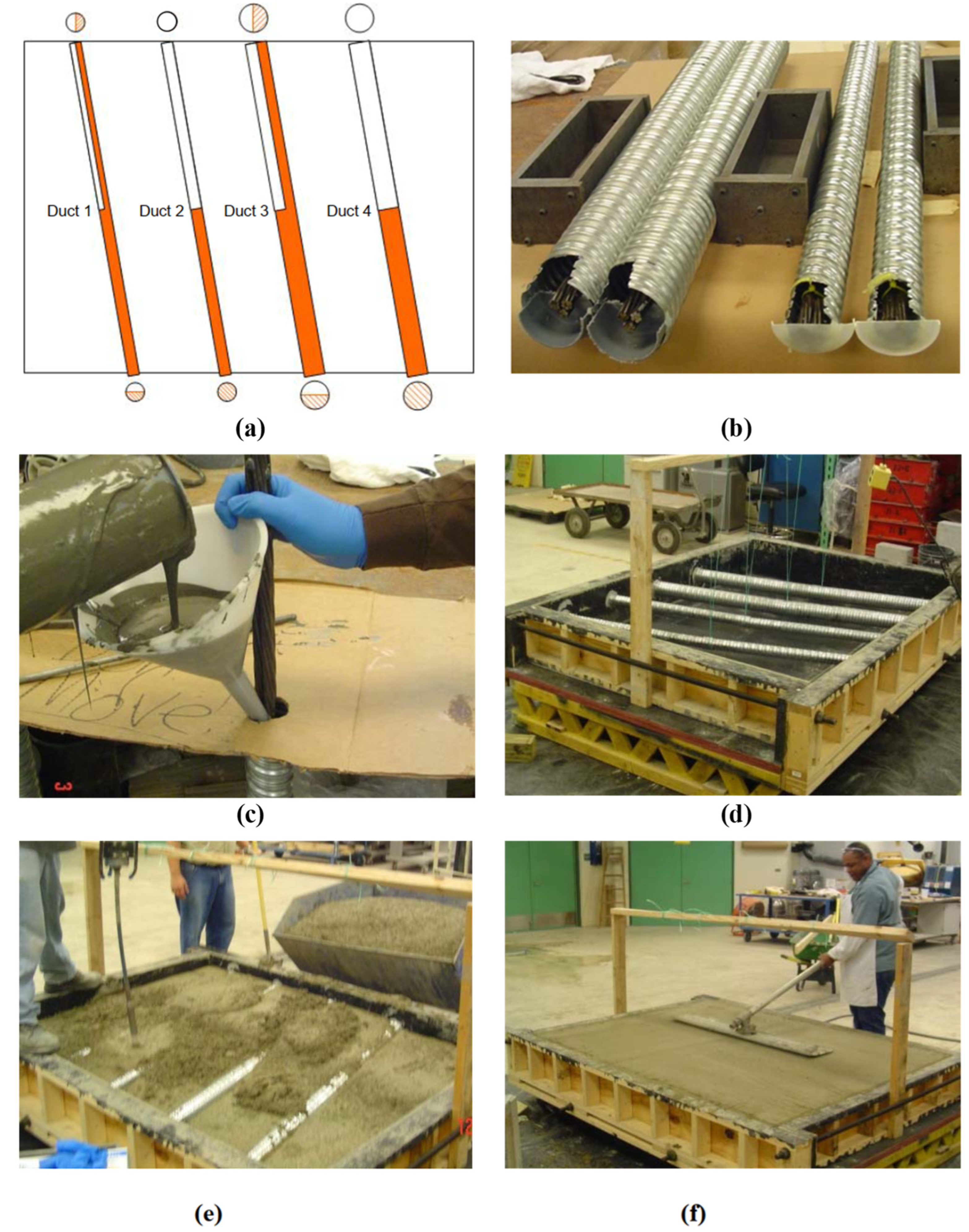
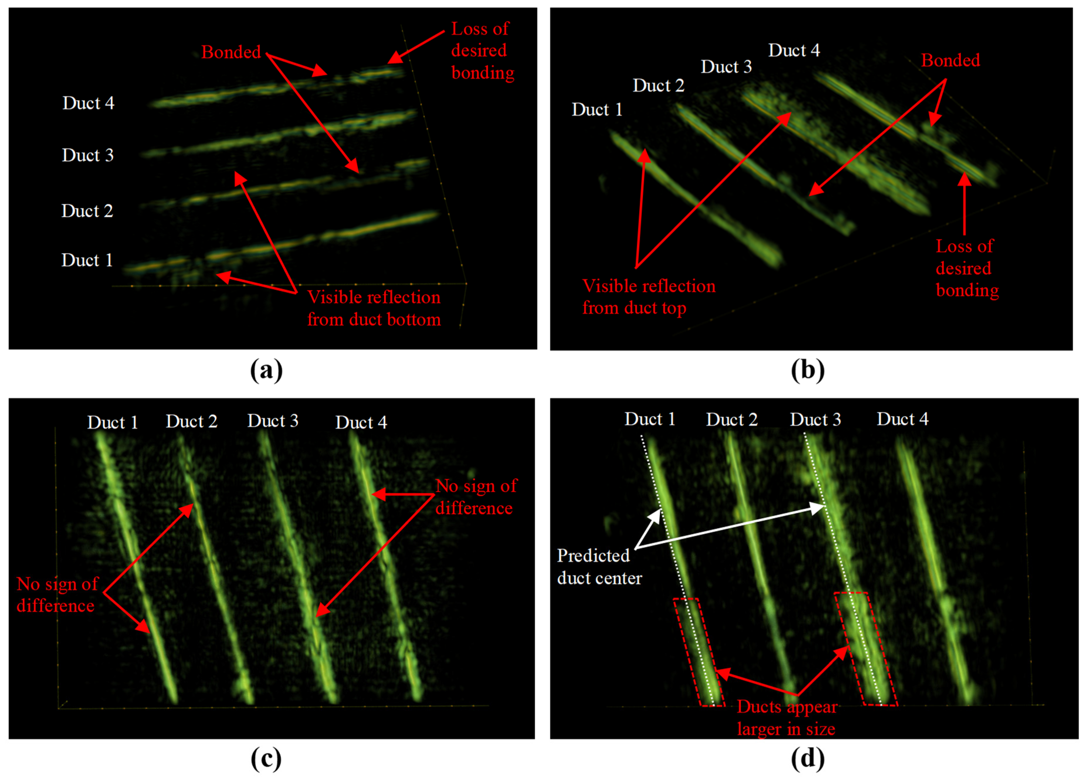
5.2.5. Slab with Metal Ducts

The slab described in this section (slab 7) was fabricated in the course of a research project sponsored by the Florida Department of Transportation. While the details of its design and construction can be found in the final report of that study [46], some general information about the slab is as follows. As depicted in Figure 14, the slab contains four metal ducts of two different sizes (two ducts per size) that are partially grouted. They have a nominal inner diameter of 50 mm and 75 mm and each of them contains three prestressing steel strands, which are not under tension. Furthermore, each duct is divided into two sections, each of which has the same grouting condition along its length. As one might realize, the objective of such a design was to create different orientations of void (grout defect). To be specific, with access to both sides of the slab (top and bottom), one can study a void that lies before, after, or alongside grout. MIRA 3D Pro was used to scan both sides of the slab in 3D/matrix mode. The imaging results with the 3D-SAFT algorithm are described and discussed in the subsequent paragraphs.

To start, Figure 15 presents the imaging results for both datasets (i.e., data collected from the top and bottom of the slab), which excluded the backwall reflection. Specifically, Figure 15a,c show the same 3D image obtained from the data collected on top of the slab but from different perspectives. Similarly, Figure 15b,d correspond to the data collected from the slab bottom. In the following, those images are evaluated in terms of their capability to differentiate (1) a fully grouted from an empty duct, (2) a partially grouted from an empty and fully grouted duct. It is noted that, when doing so, one should take into account the orientation of a void in a partially grouted duct. Specifically, counting from the scan surface, the void may be before, after, or alongside the grout. Considering the wave propagation ray path, one might predict that the signals collected in the first scenario would not show much difference from those collected for an empty duct. Such predictions and similar hypotheses are examined in turn as follows.

As to the first of the three items in the aforementioned list, one can observe a clear segmentation of duct 2 in both Figure 15a,b where the fully grouted section of the duct appears to be further away from the scanning surface than the empty section. This can be attributed to the reflection from the lower boundary of the duct, which was enabled by the presence of the grout. Based on the design of the slab, the same should be expected for duct 4. However, as indicated in the images obtained from both datasets (Figure 15a,b), such a shift only occurs for a segment of the “so-designed” fully grouted section. That said, it is very likely that the desired bonding in that section has been lost partially along the length. This hypothesis is more reasonable than the one in [46], which simply assumed a full debonding between the grout and the duct wall.

For the second item, as predicted, Figure 15c indicates no clear sign of a difference between empty and partially grouted ducts whose void is facing toward the scan surface. However, when those voids are facing away from the scan surface (bottom scan), clear effects can be observed in Figure 15d. Specifically, the ducts appear to be larger compared to both empty and fully grouted sections. The most likely explanation for this is a dominance of reflection from the grout/air interface over those from concrete/duct-wall and duct-wall/grout interfaces. Since the grout/air boundary, in this case, is linear, parallel to the scan surface, and has a size equal to the inner diameter of the duct, it should appear larger than the top portion of the duct wall when applying the SAFT imaging algorithm. Regarding the section of the duct with the void facing sideways, the evaluation was done by first plotting the ducts’ centerline as shown in Figure 15d. It is apparent that plotting was performed by extending the centerline of the symmetric section of the ducts (lower/highlighted section of duct 1 and duct 3), assuming that the ducts are perfectly linear. With those centerlines, one can easily see in Figure 15d the effect of the void facing sideways for the top section of duct 1 and duct 3. In addition, another indication of a partially grouted duct with a void facing sideways is that one can still see a weak reflection from the further side of the duct wall. Such reflection can be seen in Figure 15a,b.

6. Conclusions

Concrete imaging problems are frequently encountered in construction industry practice. These may be the simple task of locating rebars within a structure or involve a more difficult assignment of visualizing internal defects. Although invented and commercialized much later than GPR, ultrasonic shear wave devices have now proven to be a must-have for concrete imaging researchers and/or companies. Despite their popularity, the technologies employed by these devices are still not well understood by many, even advanced engineers, and senior researchers. As a consequence, ultrasonic shear wave equipment may be misused and be considered ineffective. That said, this paper was prepared and written in the form of a review report, which summarized historical developments, technologies being employed, and the main features of the devices. More importantly, laboratory experiments were used to illustrate and explain the capability of the devices. From the results presented in this paper, it is evident that ultrasonic shear wave tomography is one of the most powerful technologies for imaging concrete structures. However, it is still expected that the technology will be developed further so that it can address many more concrete imaging problems in the future.

References

1. Popovics, J.S.; Roesler, J.R.; Bittner, J.; Amirkhanian, A.N.; Brand, A.S.; Gupta, P.; Flowers, K. Ultrasonic Imaging for Concrete Infrastructure Condition Assessment and Quality Assurance; Illinois Center for Transportation: Rantoul, IL, USA, 2017. [Google Scholar]
2. Aldo, O.; Samokrutov, A.A.; Samokrutov, P.A. Assessment of concrete structures using the Mira and Eyecon ultrasonic shear wave devices and the SAFT-C image reconstruction technique. Constr. Build. Mater. 2013, 38, 1276–1291. [Google Scholar]
3. Sansalone, M.; Carino, N.J. Impact-Echo: A Method for Flaw Detection in Concrete Using Transient Stress Waves; US Department of Commerce, National Bureau of Standards, Center for Building Technology, Structures Division: Washington, DC, USA, 1986. [Google Scholar]
4. Shvaldykin, V.G.; Yakovlev, N.N. Material for the Damper of the Ultrasonic Transducer. USSR Patent SU 1280535 A1, 30 November 1986. [Google Scholar]
5. Kozlov, V.N.; Shevaldykin, V.G.; Yakovlev, N.N. Ultrasonic Low-Frequency Piezoelectric Transducer. USSR Patent SU 1425534 A1, 23 September 1988. [Google Scholar]
6. Kozlov, V.N.; Shevaldykin, V.G.; Yakovlev, N.N. Experimental Evaluation of Ultrasonic Attenuation in Concrete. Defectoscopy 1988, 2, 67–75. [Google Scholar]
7. Kovalev, A.V.; Shevaldykin, V.G.; Kozlov, V.N.; Yakovlev, N.N. Some problems in the development of the ultrasonic echo method for testing materials and products. Instrum. Control Syst. 1988, 5, 18. [Google Scholar]
8. Kozlov, V.N.; Shevaldykin, V.G.; Yakovlev, N.N. Ultrasonic Piezo Transducer. USSR Patent SU 1388785 A1, 15 April 1988. [Google Scholar]
9. Kozlov, V.N.; Samokrutov, A.A.; Yakovlev, N.N.; K.A.V.; Shevaldykin, V.G. Acoustic B- and C-tomography of coarse-grained materials by a pulsed echo method. Devices Control Syst. 1989, 7, 21–24. [Google Scholar]
10. Kovalev, A.V.; Kozlov, V.N.; Samokrutov, A.A.; Shevaldykin, V.G.; Yakovlev, N.N. Pulse echo method for testing concrete. Interference and spatial selection. Defectoscopy 1990, 2, 29–41. [Google Scholar]
11. Kozlov, V.N.; Samokrutov, A.A.; Shevaldykin, V.G. Ultrasonic Antenna Array in the Form of a Two-Dimensional Matrix. The USSR Federation Patent 2,080,592, 27 May 1997. [Google Scholar]
12. Shevaldykin, V.G.; Samokrutov, A.A.; Kozlov, V.N. Ultrasonic low-frequency short-pulse transducers with dry point contact. Development and application. In Proceedings of the International Symposium Non-Destructive Testing in Civil Engineering (NDT-CE), Berlin, Germany, 16–19 September 2003. [Google Scholar]
13. Kozlov, V.N.; Samokrutov, A.A.; Shevaldykin, V.G. Ultrasonic Low-Frequency Transducer. The USSR Federation Patent 2,082,163, 20 June 1997. [Google Scholar]
14. Shevaldykin, V.G.; Samokrutov, A.A.; Kozlov, V.N. New instrumental and methodological possibilities of ultrasonic sounding of composites and plastics. Factory laboratory. Diagn. Mater. 1998, 64, 29–39. [Google Scholar]
15. Shevaldykin, V.G.; Kozlov, V.N.; Samokrutov, A.A. Inspection of concrete with an ultrasonic echo-pulse tomograph with dry contact. Control. Diagn. 1998, 1, 49–51. [Google Scholar]
16. VShevaldykin, G.; Samokrutov, A.A.; Kozlov, V.N. Transverse ultrasonic waves in pulse echo flaw detection of pipeline support concrete. In Proceedings of the 3rd International Conference. “Diagnostics of Pipelines”, Moscow, Russia; 2001. [Google Scholar]
17. Flaherty, J.J.; Erikson, K.R.; van Lund, M. Synthetic Aperture Ultrasonic Imaging Systems. U.S. Patent 3,548,642, 22 December 1970. [Google Scholar]
18. Langenberg, K.J.; Berger, M.; Kreutter, T.; Mayer, K.; Schmitz, V. Synthetic aperture focusing technique signal processing. NDT Int. 1986, 19, 177–189. [Google Scholar] [CrossRef]
19. Martinez, O.; Parrilla, M.; Izquierdo, M.A.G.; Ullate, L.G. Application of digital signal processing techniques to synthetic aperture focusing technique images. Sens. Actuators A Phys. 1999, 76, 448–456. [Google Scholar] [CrossRef]
20. Spies, M.; Rieder, H. Synthetic aperture focusing of ultrasonic inspection data to enhance the probability of detection of defects in strongly attenuating materials. NDT E Int. 2010, 43, 425–431. [Google Scholar] [CrossRef]
21. Spies, M.; Rieder, H.; Dillhöfer, A.; Schmitz, V.; Müller, W. Synthetic aperture focusing and time-of-flight diffraction ultrasonic imaging—Past and present. J. Nondestruct. Eval. 2012, 31, 310–323. [Google Scholar] [CrossRef]
22. Mayer, K.; Marklein, R.; Langenberg, K.J.; Kreutter, T. Three-dimensional imaging system based on Fourier transform synthetic aperture focusing technique. Ultrasonics 1990, 28, 241–255. [Google Scholar] [CrossRef]
23. Krause, M.; Mielentz, F.; Milman, B.; Müller, W.; Schmitz, V.; Wiggenhauser, H. Ultrasonic imaging of concrete members using an array system. NDT E Int. 2001, 34, 403–408. [Google Scholar] [CrossRef]
24. Schickert, M.; Krause, M.; Muller, W. Ultrasonic imaging of concrete elements using reconstruction by synthetic aperture focusing technique. J. Mater. Civ. Eng. 2003, 15, 235–246. [Google Scholar] [CrossRef]
25. Tong, J.H.; Chiu, C.L.; Wang, C.Y. Improved synthetic aperture focusing technique by Hilbert-Huang transform for imaging defects inside a concrete structure. IEEE Trans. Ultrason. Ferroelectr. Freq. Control 2010, 57, 2512–2521. [Google Scholar] [CrossRef]
26. Ganguli, A.; Rappaport, C.M.; Abramo, D.; Wadia-Fascetti, S. Synthetic aperture imaging for flaw detection in a concrete medium. NDT E Int. 2012, 45, 79–90. [Google Scholar] [CrossRef]
27. Shokouhi, P.; Wolf, J.; Wiggenhauser, H. Detection of delamination in concrete bridge decks by joint amplitude and phase analysis of ultrasonic array measurements. J. Bridge Eng. 2014, 19, 04013005. [Google Scholar] [CrossRef]
28. Tong, J.H.; Chiu, C.L.; Wang, C.Y.; Liao, S.T. Influence of rebars on elastic-wave-based synthetic aperture focusing technique images for detecting voids in concrete structures. NDT E Int. 2014, 68, 33–42. [Google Scholar] [CrossRef]
29. Bittner, J.A.; Spalvier, A.; Popovics, J.S. Internal imaging of concrete elements. Concr. Int. 2018, 40, 57–63. [Google Scholar]
30. Lin, S.; Shams, S.; Choi, H.; Azari, H. Ultrasonic imaging of multi-layer concrete structures. NDT E Int. 2018, 98, 101–109. [Google Scholar] [CrossRef]
31. Dinh, K.; Gucunski, N.; Zayed, T. Automated visualization of concrete bridge deck condition from GPR data. NDT E Int. 2019, 102, 120–128. [Google Scholar]
32. Dinh, K.; Gucunski, N.; Tran, K.; Novo, A.; Nguyen, T. Full-resolution 3D imaging for concrete structures with dual-polarization GPR. Autom. Constr. 2021, 125, 103652. [Google Scholar]
33. VKozlov, N.; Samokrutov, A.A.; Shevaldykin, V.G. Thickness measurements and flaw detection in concrete using ultrasonic echo method. Nondestruct. Test. Eval. 1997, 13, 73–84. [Google Scholar] [CrossRef]
34. Hoegh, K.; Khazanovich, L.; Yu, H.T. Ultrasonic tomography for evaluation of concrete pavements. Transp. Res. Rec. 2011, 2232, 85–94. [Google Scholar] [CrossRef]
35. Vancura, M.; Khazanovich, L.; Barnes, R. Concrete Pavement Thickness Variation Assessment with Cores and Nondestructive Testing Measurements. Transp. Res. Rec. 2013, 2347, 61–68. [Google Scholar] [CrossRef]
36. Chen, R.; Tran, K.T.; Dinh, K.; Ferraro, C.C. Evaluation of Ultrasonic SH-Waveform Tomography for Determining Cover Thickness and Rebar Size in Concrete Structures. J. Nondestruct. Eval. 2022, 41, 1–16. [Google Scholar] [CrossRef]
37. Chen, R.; Tran, K.T.; La, H.M.; Rawlinson, T.; Dinh, K. Detection of delamination and rebar debonding in concrete structures with ultrasonic SH-waveform tomography. Autom. Constr. 2022, 133, 104004. [Google Scholar]
38. Jana, D. Delamination—A State-of-the-art Review. In Proceedings of the Twenty-Ninth Conference on Cement Microscopy, Quebec City, QC, Canada, 20–24 May 2007. [Google Scholar]
39. Shokouhi, P.; Wöstmann, J.; Schneider, G.; Milmann, B.; Taffe, A.; Wiggenhauser, H. Nondestructive detection of delamination in concrete slabs: Multiple-method investigation. Transp. Res. Rec. 2011, 2251, 103–113. [Google Scholar] [CrossRef]
40. Nguyen, T.D.; Tran, K.T.; Gucunski, N. Detection of bridge-deck delamination using full ultrasonic waveform tomography. J. Infrastruct. Syst. 2017, 23, 04016027. [Google Scholar]
41. Choi, P.; Kim, D.H.; Lee, B.H.; Won, M.C. Application of ultrasonic shear-wave tomography to identify horizontal crack or delamination in concrete pavement and bridge. Constr. Build. Mater. 2016, 121, 81–91. [Google Scholar] [CrossRef]
42. Clayton, D.A.; Smith, C.M.; Ferraro, C.C.; Nelson, J.; Khazanovic, L.; Hoegh, K.; Chintakunta, S.; Popovics, J.; Choi, H.; Ham, S. Evaluation of Ultrasonic Techniques on Concrete Structures; Oak Ridge National Laboratory: Oak Ridge, TN, USA, 2013. [Google Scholar]
43. Terzioglu, T.; Karthik, M.M.; Hurlebaus, S.; Hueste, M.B.D.; Maack, S.; Woestmann, J.; Wiggenhauser, H.; Krause, M.; Miller, P.K.; Olson, L.D. Nondestructive evaluation of grout defects in internal tendons of post-tensioned girders. NDT E Int. 2018, 99, 23–35. [Google Scholar] [CrossRef]
44. Shin, S.W.; Zhu, J.; Min, J.; Popovics, J.S. Crack depth estimation in concrete using energy transmission of surface waves. ACI Mater. J. 2008, 105, 510. [Google Scholar]
45. Lin, S.; Wang, Y. Crack-Depth estimation in concrete elements using ultrasonic shear-horizontal waves. J. Perform. Constr. Facil. 2020, 34, 04020064. [Google Scholar] [CrossRef]
46. Hiltunen, D.R.; Algernon, D.; Ferraro, C.C. Validation of Nondestructive Testing Equipment for Concrete; University of Florida: Gainesville, FL, USA, 2010. [Google Scholar]
Figure 1. Preliminary transducer array with liquid contact (courtesy of ACS Group).
Infrastructures 08 00053 g001
Figure 2. Various versions of ultrasonic shear wave devices (courtesy of ACS Group).
Infrastructures 08 00053 g002
Figure 3. Effects of array polarization: (a) the reflecting object is parallel to the transducers and (b) the point object or object perpendicular to the transducers.
Infrastructures 08 00053 g003
Figure 4. Measuring concrete thickness from the B-scan image.
Infrastructures 08 00053 g004
Figure 5. Slab 1 and Slab 2: (a) before and (b) after casting.
Infrastructures 08 00053 g005
Figure 6. Imaging results for slab 1 and slab 2: (a,b) 3D images, (c,d) B-scan images, (e,f) side-view photos with ground-truth dimensions.
Infrastructures 08 00053 g006
Figure 7. Slab 3 and Slab 4: (a) before and (b) after casting.
Infrastructures 08 00053 g007
Figure 8. Imaging results for slab 3 and slab 4: (a,b) 3D images, (c,d) B-scan images, (e,f) side-view photos.
Infrastructures 08 00053 g008
Figure 9. Slab 5: (a) before casting and (b) photo of MIRA data collection.
Infrastructures 08 00053 g009
Figure 10. Imaging results for slab 5 from different view angles (a,c) versus ground truth (b,d).
Infrastructures 08 00053 g010
Figure 11. Slab 6: (a) 3D rendering, (b) before casting, (c) installing pervious concrete prism, (d) installing wet-sieved concrete into the surface to more realistically simulate poor consolidation, (e) view of finished slab bottom [42], (f) view of survey grid.
Infrastructures 08 00053 g011
Figure 12. Imaging results for slab 6 from different view angles (a,b) versus ground truth (c,d).
Infrastructures 08 00053 g012
Figure 13. Effect of crack depth on backwall visualization.
Infrastructures 08 00053 g013
Figure 14. Slab 7: (a) schematic design, (b) preparing duct, (c) filling the grout, (d) installing the ducts in formwork, (e) concrete placement, (f) finishing the concrete surface [46].
Infrastructures 08 00053 g014
Figure 15. Images for slab 7 from: (a) top scan, (b) bottom scan, (c) top scan, (d) bottom scan.
Infrastructures 08 00053 g015
Disclaimer/Publisher’s Note: The statements, opinions and data contained in all publications are solely those of the individual author(s) and contributor(s) and not of MDPI and/or the editor(s). MDPI and/or the editor(s) disclaim responsibility for any injury to people or property resulting from any ideas, methods, instructions or products referred to in the content.