Article

On a Benchmark Problem for Modeling and Simulation of Concrete Dams Cracking Response

by
Paulo Marcelo Vieira Ribeiro
1,* and
Pierre Léger
2
1
Departamento de Engenharia Civil e Ambiental, Universidade Federal de Pernambuco, Recife 50740-530, Brazil
2
Département des Génies Civil, Géologique et des Mines, École Polytechnique de Montréal, Montréal, QC H3C 3A7, Canada
*
Author to whom correspondence should be addressed.
Infrastructures 2023, 8(3), 50; https://doi.org/10.3390/infrastructures8030050
Submission received: 6 February 2023 / Revised: 1 March 2023 / Accepted: 5 March 2023 / Published: 9 March 2023
(This article belongs to the Special Issue Advances in Dam Engineering of the 21st Century)

Abstract

:
Concrete dams are massive unreinforced quasi-brittle structures prone to cracking from multiple causes. The structural safety assessment of cracked concrete dams is typically performed using computational analysis through numerical methods, with adequate representation of the material model. Advances in the last decades including computational processing power, novel material, and numerical models have enabled remarkable progress in the analysis of concrete dams. Nevertheless, classical benchmarks remain reliable references for the performance analysis of these structures. This paper presents the main aspects of modeling and simulation of a concrete gravity dam cracking response based on a broad literature survey. Emphasis is given to an in-depth review of the benchmark problem analyzed by Carpinteri et al. (1992). We then use the Abaqus concrete damage plasticity constitutive model to solve the benchmark problem and provide recommendations to obtain accurate results with an optimal computational cost. The best practices of modeling, simulation, verification, and validation are presented.

1. Introduction

Concrete dams are massive unreinforced quasi-brittle structures prone to cracking from multiple causes under normal and extreme operating conditions such as floods and earthquakes [1,2,3,4,5,6,7,8]. The structural safety assessment of cracked concrete dams is typically performed using finite element (FE) numerical modeling and simulation of crack initiation and propagation to establish a critical crack pattern and quantify the associated residual strength. A crack introduces a geometric discontinuity in the displacement field that alters the stiffness and load-carrying capability of the dam. The stress singularity at the crack tip leads to infinite stresses when using the elasticity theory. The definition of suitable concrete FE constitutive models and numerical solution algorithms to quantify crack patterns and circumvent the stress singularity problem, using fracture mechanics and nonlinear FE solution algorithms, is still the subject of active research. Discrete crack models [9,10,11,12,13], smeared crack continuum models [1,3,14,15,16] and boundary element techniques [5,8,17,18] have been developed by various researchers with varying degrees of success. Commercial FE software packages such as Abaqus, ANSYS, DIANA, VecTor, MIDAS, ATENA, and LS-Dyna also offer some concrete cracking constitutive models that require an advanced level of expertise to be used reliably.
The development, implementation, and confident use of FE concrete constitutive models require rigorous verification and validation procedures. One must distinguish between verification and validation. According to [19] verification is defined as “the process of determining that a model implementation accurately represents the developer’s conceptual description of the model and the solution to the model”. Verification deals with mathematical issues (that is, “solving the equation right”), such as code verification (removing mistakes and errors) as well as the verification of the accuracy of the numerical solution [20]. On the other hand, solution validation is defined as “the process of determining the degree to which a model is an accurate representation of the real world from the perspective of the intended uses of the model”. Validation deals with the physics of the problem, that is “solving the right equations” for an accurate solution to the engineering problem considered. Validation also aims at improving the fundamental understanding and mathematical models of the physics at hand (i) by characterizing and minimizing uncertainties and possible limitations or errors in the computational model and experimental data, and (ii) by increasing the confidence in the quantitative predictive ability of the computational model. Validation usually follows a hierarchical methodology where benchmarking against experimental data plays a fundamental role.
Obviously, one cannot test the failure of a full-scale dam-foundation-reservoir system because of the scale at which physical phenomena are occurring and the nature of extreme loadings such floods and earthquakes. Some laboratory tests on small-scale dams have been published from time to time to validate concrete constitutive models. One of these tests, shown in Figure 1 and Figure 2, performed on a 1:40 scale-down model was published in [9] and has been widely used as a benchmark problem for concrete constitutive model validation by several researchers [1,2,3,4,5,6,7,8,10,11,12,13,14,15,16,17,18,21,22,23,24,25,26,27,28,29]. It is expected that this benchmark problem will still be used in the future as new constitutive and numerical methods are developed.
In this paper we first critically review the benchmark problem presented in [9] with an extensive literature review comparing results that were published using (i) FE discrete crack models, (ii) FE continuum models with or without enhancement (XFEM), and (iii) boundary elements, particle, and meshfree models. We then use the Abaqus [30] concrete damage plasticity constitutive model to solve the benchmark problem and provide recommendations to obtain accurate results with an optimal computational cost, exploring the incidence of (i) mesh size, (ii) type of elements, (iii) material properties, (iv) tensile softening behavior, (v) solution algorithm, and (vi) local mesh refinement.

2. Carpinteri Gravity Dam Models—Literature Survey

The original investigation in [9] focused on the crack propagation behavior in concrete gravity dams using reduced-scale tests and cohesive crack numerical models. This is probably one of the earliest research works developed at Politecnico di Torino for the experimental analysis of cracking in concrete dams, as discussed in [13]. Although additional experimental results are available from other benchmarks, the following discussion will focus on the model and results obtained from the former reference. The experimental and numerical results of this research have been extensively analyzed by several authors, providing key aspects that are presented in the subsequent sections.

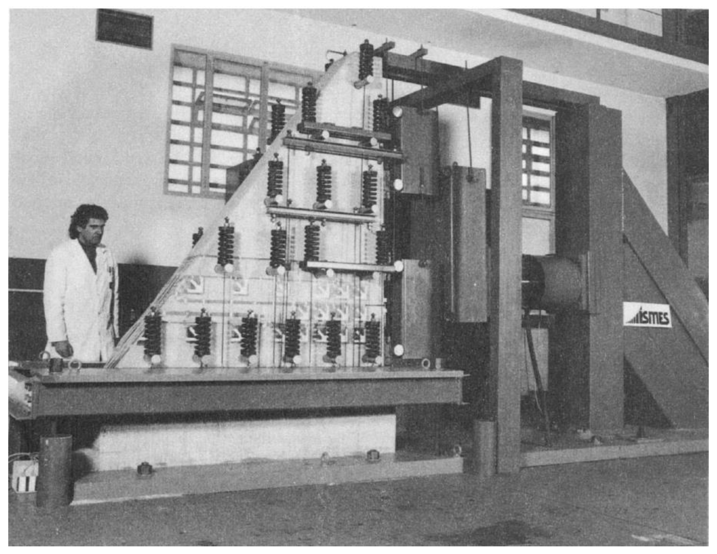
2.1. The Experimental-Numerical Study Developed at Politecnico di Torino

This benchmark consists of a reduced-scale dam section (1:40) analyzed in [9], depicted in Figure 1, using laboratory and numerical tests, where an imposed notch is located at the upstream face. Two scenarios were analyzed, including notch-depth ratios of 0.1 and 0.2, positioned at a quarter of the dam height. This experimental setup included self-weight (by means of equivalent vertical forces distributed on the monolith plane), and equivalent horizontal hydrostatic loads (by means of four actuators positioned at the upstream side). Displacement control CMOD (Crack Mouth Open Displacement) was a key parameter in this setup, acting as feedback for the servocontrolled actuators. A summary of the cases described in the experimental setup is presented in Table 1.
The reference FE results were also presented by the authors. The numerical model consisted of a bidimensional mesh of 6-node quadratic triangular elements. The material nonlinearity was considered by means of a cohesive crack model. An interesting approach was applied using automatic remeshing to consider the crack growth trajectory. This strategy considered the crack tip advance based on the evaluation of the component of displacement discontinuity normal to the crack surface. Because the initial crack trajectory was not known a priori, a remeshing scheme was proposed, considering each crack growth step. The threshold was set to the value of the displacement component associated with the occurrence of normal cohesive stress equal to zero, and a linear constitutive law described the behavior of tensioned concrete. The authors concluded that the proposed numerical model was able to reproduce the results of the experimental setup with an acceptable degree of accuracy. Results for crack trajectories were also retrieved from the numerical models, including their association with the pattern observed in the reduced-scale model.

2.2. A Survey of Analyses Presented by Several Authors

Carpinteri et al.’s [9] studies were reproduced by several authors, using diverse numerical methods. This section provides a survey of most of these contributions, including a summary of the key findings of past research.

2.2.1. Analyses Considering Finite Elements with Discrete Crack Models

Valente and Barpi [10] investigated the cohesive crack model for the transition of ductile to brittle behavior and analyzed the singularity of the stiffness matrix and the stability of the crack trajectory. For these analyses the crack trajectory is generally not known a priori and a remeshing scheme is required for each fictitious crack growth step. Their results indicate that different options for the crack tip position provide distinct results for crack trajectories and load-CMOD plots.
Barpi [11] presented a detailed discussion for Carpinteri et al.’s [9] experimental analysis, including results which considered linear and bilinear concrete softening laws, as well as comparison with different numerical methods. Investigations were performed for the original two notch-depth ratios of 0.1 and 0.2. Load-CMOD results indicated that peak loads for bilinear softening models are reduced when compared to linear models. Conversely, crack trajectories are almost convergent, regardless of the softening model.
Barpi and Valente [12] analyzed three reduced-scale dam models (1:40, 1:100, 1:150), considering the influence of two notch-depth ratios: 0.1 and 02. Load-CMOD curves and crack trajectories are represented satisfactorily with numerical computations. Relevant considerations are presented for the need for physical similarity in the experimental models, including the scaling of fracture energy.
Carpinteri et al. [13] presented an extensive review of past research developed at Politecnico di Torino. The authors provide a discussion of early studies involving the cohesive crack model, which is based on the separation of adjacent nodes belonging to a crack trajectory. Limitations involving the size scale and the need for special requirements for the analysis of unnotched specimens are also verified.
Shi et al. [2] analyzed two different models including single and multiple-crack propagation. These models are based on a bilinear strain softening relation defined by Rokugo et al. [31], which is applied to the crack equations. An efficient remeshing scheme is proposed with the use of triangular finite elements. Crack trajectories are mostly horizontal under the mode-I hypothesis. A discussion is provided about limitations in the experimental results.
Shi [21] presented an updated formulation considering a mixed-mode (mode-I and mode-II) fracture. Crack trajectories are similar for mode-I and mixed-mode but differ once the shear transfer mechanisms become relevant. Results for load-CMOD curves are not provided.
Lohrasbi and Attarnejad [22] presented results using both discrete and smeared crack finite element models. The authors concluded that the latter is efficient in terms of computational cost but provides unreliable results.
Wu et al. [23] proposed a mixed-mode (mode-I and mode-II) method with comparisons to experimental tests and past results by Barpi and Valente [12], including their study of two different notch-depth ratios. The numerical results for crack trajectories agree with the experimental observations. This method requires the definition of the initial cracking toughness and provides an accurate estimate of the ultimate bearing capacity.
Table 2 presents a summary of relevant information for benchmark purposes considering the finite elements with discrete crack models.

2.2.2. Continuum Models Considering Smeared Crack and Enhanced Finite Elements

Bhattacharjee and Léger [1] proposed a numerical implementation of smeared crack models in 4-node isoparametric finite elements by means of two constitutive frameworks: coaxial rotating crack model (CRCM) and fixed crack model with a variable shear resistance factor (FCM-VSRF). The authors concluded that the procedure is an efficient strategy in terms of computational cost, avoiding remeshing steps. However, a stiffer post-peak response is observed.
Ghrib and Tinawi [14] proposed a finite element method implementation defined as DAM-MEC (damage mechanics analysis of concrete dams) using three different damage models, with isotropic and anisotropic behavior. Isotropic models provide horizontal crack trajectories. Stress locking is overcome using a fixed angle of damage direction in the anisotropic model. Localized damage is observed at the dam’s heel.
Oliver et al. [24] presented the theoretical aspects and a series of applications concerning a finite element implementation of a fracture mechanics model. This concept is defined as a strong discontinuity approach (SDA), without the necessity of any remeshing procedure and avoiding mesh bias drawbacks.
Mirzabozorg and Ghaemian [3] studied a smeared crack model for 3D static and dynamic behavior of mass concrete. A finite element implementation is performed using a 20-node isoparametric element with a coaxial rotating crack model. Stress locking is observed for load-CMOD curves. Crack trajectories are mostly horizontal. It also verified the presence of a plastic region at the dam’s heel.
Cai [15] proposed a finite element implementation using a smeared crack approach. Analysis results are limited to the peak value of the load-CMOD plot and stress locking limitations are also discussed.
Hariri-Ardebili et al. [4] investigated a coaxial rotating smeared crack model in 3D. Load-CMOD curve presents a reliable approximation to the reference results, but crack trajectories are not analyzed.
Roth et al. [25] and Wang et al. [6] applied a novel technique considering the continuum approach for the first stages of cracking and the discrete nature of the Extend Finite Element Method (XFEM) for macroscopic cracks. Load-CMOD and crack trajectory results are presented and compared to reference data provided by Carpinteri et al. [9].
Dias et al. [7] proposed a procedure defined as crack-path-field and strain injection, where finite elements are enhanced in a similar fashion to XFEM, avoiding mesh bias presented in standard displacement-based formulations. This technique provides specific strain fields within the elements for capturing and propagating strain localization. The position of this injection is determined by a crack-path-field algorithm. Results for the load-CMOD curve are in excellent agreement with Carpinteri et al.’s [9] data.
Durieux and Rensburg [16] discussed the use of nonlinear FEM analyses based on the Drucker-Prager material model to overcome the problem of stress peaks at singularity points and to produce a more realistic stress distribution in concrete dams. A simulation was performed for Carpinteri et al.’s [9] benchmark. The load-CMOD analysis is limited to the peak load and no post-peak information is provided. Nevertheless, peak load values are consistent with the reference results. The development of plastic strains at the model’s base is noticeable.
Sha and Zang [26] presented analyses dedicated to the problem hydraulic fracture in concrete dams by means of damage mechanics models. Some benchmark results are presented for uncoupled models, consisting of crack trajectory and load-CMOD curve. The latter is in excellent agreement with the experimental data but presents a stiffer pre-peak response when compared to Barpi and Valente’s [12] data.
Table 3 presents a summary of past research data for benchmark [9] considering the finite elements with continuum models.

2.2.3. Analyses Considering Conventional and Enhanced Boundary Elements

Chahrour and Ohtsu [17] studied a Boundary Element Method (BEM) approach with the notch being defined by a stitching interface which follows the expected crack trajectory. Four linear elastic fracture mechanics criteria were applied for different simulations. The crack trajectories predicted by the BEM are acceptable when compared to experimental results. However, an uncommon behavior is shown by the load-CMOD curve, which displays a series of snapbacks in the early stages of crack propagation.
Shi et al. [5] presented an investigation of crack propagation by means of boundary polygons, which model the linear elastic bulk concrete. These regions are coupled with interface elements, which model the fracture zone between crack faces. This strategy consists of applying the Scaled Boundary Finite Element Method (SBFEM). A detailed discussion is presented for the theoretical background of this method, and its integration with a cohesive crack model. Results for coarse, medium, and fine meshes are almost identical when analyzing the load-CMOD curves and the crack trajectories. The latter are mostly straight lines, while the experimental results presented paths directed to the dam’s toe.
Yao et al. [8] applied the SBFEM including hydraulic fracture aspects for the crack propagation in concrete dams. The results for zero water pressure at the crack were also presented and compared to the reference results provided by Carpinteri et al. [9], as well as those obtained by Barpi and Valente [12] and Shi et al. [5]. The load-CMOD curves agree with past analyses. However, crack trajectories are mostly horizontal and deviate from the experimental observations at about half length of the dam’s section.
Li et al. [18] proposed a novel model using the Extended Scale Boundary Finite Element Method (XSBFEM) with the incorporation of the cohesive fracture behavior of concrete. In this case, the discontinuous behavior at the crack is captured by means of Heaviside enrichment functions, avoiding the need for new nodes at the crack face, which is a requirement for the SBFEM. The load-CMOD curve results agree with those presented by Barpi and Valente [12], and Shi et al. [5]. The crack trajectories follow the expected 20 degrees pattern observed in the experimental setup of Carpinteri et al. [9] and present a higher fidelity when compared to past research results.
Table 4 presents a summary of relevant information for benchmark purposes considering conventional and enhanced boundary elements.

2.2.4. Analyses Considering Particle or Meshfree Methods

Attard and Tin-Loi [27] presented a new method for the analysis of concrete fracture, with a technique defined as particle/interface type models. The proposal comprised discrete units formed by an assembly of nine constant strain triangles. Cracking is represented by the opening or closing across the interfaces of these discrete units. The analysis results presented a good agreement for both the crack trajectory and load-CMOD curve, when compared to Carpinteri et al.’s [9] data.
Su et al. [28] developed a hybrid finite element-meshfree approach for the study of crack propagation in concrete dams. In this case, 3D fractured elements are enriched by a planar crack surface that is not restricted to the element faces. Analyses were performed using tridimensional models, which is quite a unique aspect in the literature survey. Load-CMOD curves are not presented, but an extensive comparison is provided for the crack trajectories, including the data provided by Carpinteri et al. [9] and Shi et al. [2]. The simulation results follow the expected 20 degrees path toward the dam’s toe.
Yang et al. [29] applied the Ordinary State Base Peridynamics (OSBPD) model for the analysis of cohesive crack growth. In this case, the Classic Continuum Mechanics (CCM) is substituted by an integral form, and the assumption of continuous displacement field in CCM is not required by the peridynamics approach. The equations are based on a model which treats the internal forces within a body as a network of interactions in the same fashion as molecular dynamics. Results for the crack trajectory and load-CMOD curve are presented and agree with the reference data presented by Carpinteri et al. [9].
Table 5 presents a summary of past research data for benchmark purposes considering conventional and enhanced boundary elements.

3. Modeling and Simulation of Carpinteri Gravity Dam Using the Abaqus CDP Model

The present section is focused on the modeling details and simulation of the experimental setup provided by Carpinteri et al. [9]. The finite element models were established using commercial software Abaqus v. 6.14-1 [30] with the so-called concrete damage plasticity model (CDP). Information related to geometry, material model, mesh, boundary conditions, interactions, and solver options is detailed in the following sections. Subsequently, the simulation results are presented and discussed.

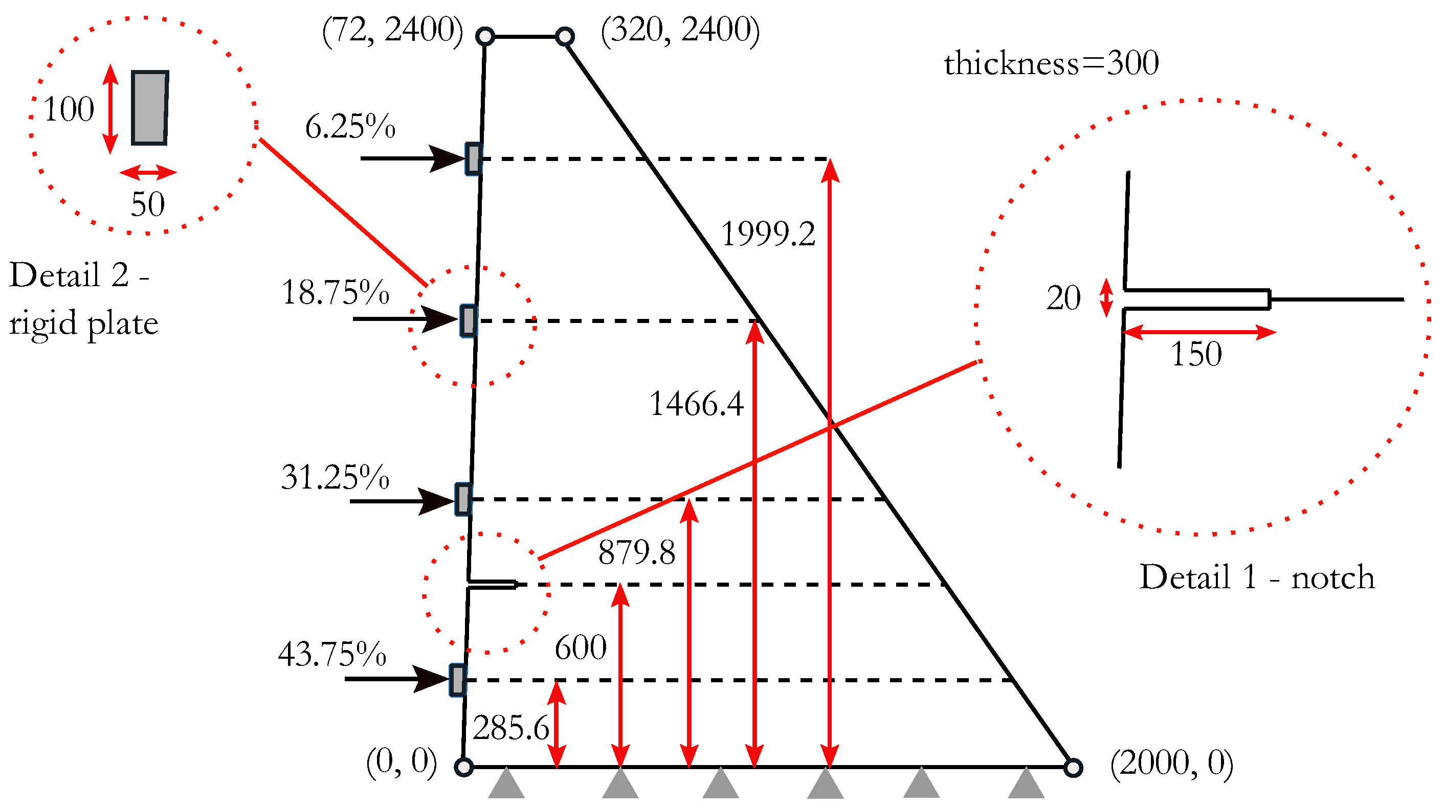
3.1. Geometry Definition

The geometry is defined as a bidimensional dam, following the same reasoning of Carpinteri et al.’s [9] numerical model. However, it should be noted that limitations arise when comparing the 2D approach with the experimental setup, which is a 3D reduced-scale gravity dam section. This experimental setup includes thickness transition at different elevations (see Figure 1), which cannot be represented in a 2D fashion. Nevertheless, the 2D approach has been extensively applied for this benchmark, and the literature survey indicates few papers using 3D models, such as Mirzabozorg and Ghaemian [3], Hariri-Ardebili et al. [4], and Su et al. [28].
The main characteristics of the geometric domain are presented in Figure 2. This idealized 2D geometry is simplified considering the removal of the first and second segments of the lower portion of the dam, with corresponding heights equal to 250 mm and 150 mm, respectively. Past research indicates that the inclusion of the first segments is seldom used, and even the numerical model presented by Carpinteri et al. [9] considers a simplified geometry which neglects this part. The inclusion of the second segment is prevalent in past research, but this part presents a variable thickness and details about the uniform thickness for the 2D representation of this segment were not found in the literature survey. It will be shown later that this is not a major concern for the finite element simulations, because the nonlinear response is highly dependent on the notch behavior, regardless of any considerations provided for the inclusion of the first and second segments.
A relevant aspect involves the inclusion of four rigid plates for load application at the dam’s upstream face. These are defined using 2D discrete rigid parts, which are coupled to the main geometry by means of tie constraints. These parts will provide a distributed load transfer region, avoiding localized stress effects.
The notch is defined by a separate part in the model and a Boolean subtraction operation is performed for the removal of the corresponding region in the dam domain. Following Carpinteri et al.’s [9] prescriptions, only the first notch-depth ratio is employed: 0.1 W, with W defining the dam width at the notch location [28]. This corresponds to Test Case 2.

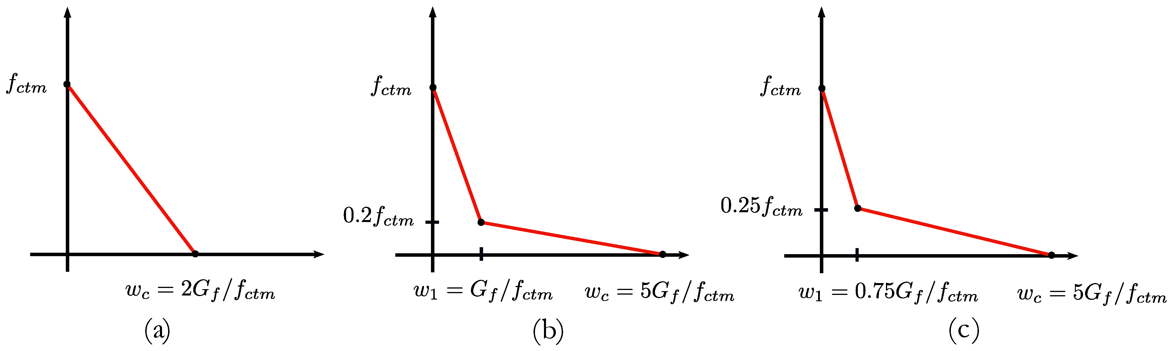
3.2. Material Properties

Data of the experimental program investigated by Carpinteri et al. [9] is given in Table 6, including the elastic modulus (E), Poisson’s ratio (v), the tensile strength (ft), and the fracture energy (Gf). Additional information includes a maximum aggregate size of 25 mm. No details are given for the compressive behavior of the concrete.
In Abaqus, the material nonlinear behavior is defined by the CDP. The main characteristics of the CDP model are the representation of concrete as a continuum, plasticity-based, damage model with major failure mechanisms described in accordance with tensile cracking and compressive crushing. By means of the flowchart presented by Ghrib and Tinawi [14], it is reasonable to assume that this strategy falls into the fixed mesh approach using isotropic damage mechanics. Therefore, no remeshing is required (positioning this analysis in the category of continuum models with finite elements, as defined in the literature survey). The microcracking under uniaxial tension is represented macroscopically by a softening portion of the stress-strain curve that initiates after the onset of the tensile failure stress, which is preceded by an initial elastic stage. For uniaxial compression, the main features of the stress-strain curve are given by an initial linear response, followed by a stress hardening stage, and finally, a softening phase that starts after the onset of the ultimate compressive stress.
For the current simulations emphasis is given only to the tensile behavior, and three different models are investigated for the stress-crack opening for uniaxial tension. These are shown in Figure 3. The first is given by a linear model, which represents a straightforward representation of the tension softening. The remaining are represented by bilinear models following the fib model code 2010 [32] and Rokugo et al.’s [31] recommendations. Those different representations share a similar aspect: the area under the softening curves is the same, preserving the fracture energy regardless of the model choice.
The damage parameter plays an important role in the CDP model and defines the degradation of the concrete elastic stiffness under an unloading scenario. This variable assumes a zero value, which represents undamaged material prior to the start of the softening stage. From that point and beyond, damage increases gradually, following stress reduction. A complete degradation is represented by Value 1.
The CDP model is also represented by a non-associated plastic flow rule that follows the Drucker-Prager hyperbolic function and a yield function defined by Lubliner et al. [33], with the modifications proposed by Lee and Fenves [34]. For the plastic flow rule, two key parameters are required by Abaqus: ψ, the dilation angle; and ε, the eccentricity. For the yield function, two key variables are necessary: σb0/σc0, the ratio of initial equibiaxial compressive yield stress to initial uniaxial compressive yield stress; and Kc, the ratio of the second stress invariant on the tensile meridian with that on the compressive meridian. Table 7 presents the details about the parameters selected for the numerical models. The dilation angle is set to 40 degrees, following typical values of past research in concrete dams [35,36]. Abaqus default values are selected for the remaining variables. The last column is related to an additional parameter available for viscoplastic regularization of the constitutive equations, which improves convergence rate in the softening regime. However, this feature was not applied in the numerical models.
The compressive behavior is defined as elastic, with a yield stress of 30 Mpa and an inelastic strain of zero value. For the tensile post-cracking behavior, Abaqus provides three different options: strain, displacement, and the mode-I fracture energy (GFI). The second is selected for the subsequent simulations, and the required stress-crack values are dependent on the tension softening model, as described previously.

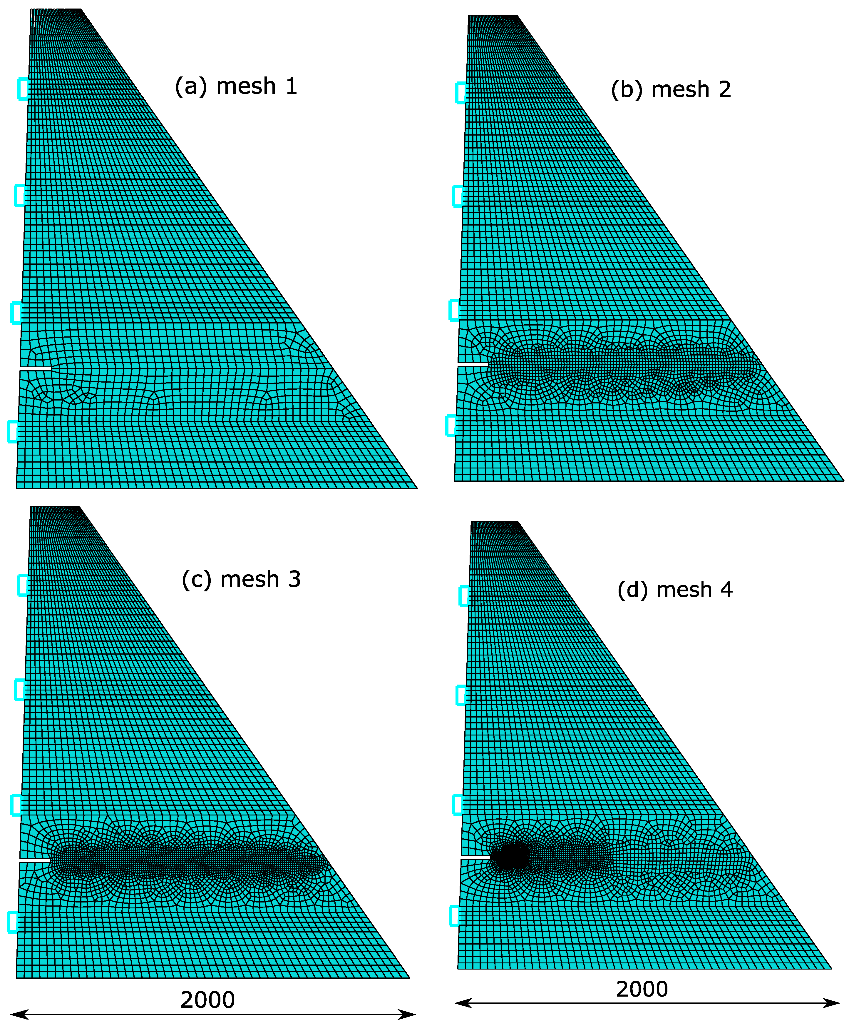
3.3. Mesh, Boundary Conditions, Interactions, and Solver Options

Analyses were defined by four different levels of refinement, which comprise unstructured meshes in the notch domain strip, and structured refinement for the remaining parts. Details are given in Figure 4. These meshes are composed of the following total number of elements: 3081 (mesh 1), 4239 (mesh 2), 5388 (mesh 3) and 5111 (mesh 4). Most of these elements are defined by CPS4R, which are 4-node, bilinear, plane stress elements with reduced integration. Some very specific regions required elements of type CPS3, which are 3-node, linear, plane stress elements. These comprise less than 2% of the total of mesh elements, independently of the refinement level. Rigid elements of type R2D2 are also present, defining the four regions for load application (as stated in the geometry definition). The first three meshes are defined by a uniform element density at the notch strip region. An exception is given by mesh 4, which is based on a progressive level of refinement, with a higher concentration of elements at the notch region, but with a reduction in the refinement level toward the downstream face. In this case, the progressive refinement is composed of three different regions, and only the vicinity of the notch is discretized with small-sized elements.
The refinement strategy was defined using a horizontal edge that starts at the midpoint of the vertical dimension of the notch and extends to the downstream face of the dam. This procedure enables an efficient refinement of the notch strip region, since the element size is defined along this edge, and automatic mesh transition is performed to the upper and lower parts of the geometry (beyond the notch strip region). Meshes 1, 2 and 3 were developed using a uniform refinement along this boundary (using Abaqus seed command), with approximate element edge sizes of 30, 15 and 10 mm, respectively. A nonuniform refinement is applied for mesh 4. For this case, the horizontal edge was divided into three different segments of approximately 14%, 32% and 54% of the total length. Progressive element sizes of 5, 10 and 20 mm were assigned to each of these segments. This enables a fine-coarse mesh transition, while still providing a fine mesh at the vicinity of the notch.
In practical terms, the notch strip region with unstructured mesh is composed of the following number of elements: 626 (coarse), 1784 (mesh 2), 2933 (mesh 3), and 2656 (mesh 4). For this specific region, the number of elements of mesh 4 is reduced when compared to mesh 3. However, the former presents a larger element concentration at the vicinity of the notch. It will be shown later that these different refinement levels enable a progressive interpretation of the cracking response, with an optimal use of the computational resources. They also enable the analysis of a possible mesh bias in each configuration.
Boundary conditions are given by nodes with restrained in-plane displacements at the foundation level, and point loads applied in the horizontal direction at the center of each corresponding rigid plate. The latter is an idealized representation of the experimental setup, which consists of the combination of a major beam that is connected to the hydraulic actuator, supported by two additional beams, that provide reactions at the upstream face of the dam (as shown in Figure 1). A more feasible approach is proposed using the arc-length method (static Riks), and the direct application of the point loads to rigid plates, providing a uniform stress distribution to the corresponding locations. These loads follow Carpinteri et al.’s [9] experimental setup, given by the following percentages of the total load, measured from bottom to top: 43.75, 31.25, 18.75 and 6.25 (as presented in Figure 2). The interaction between the rigid plates and the dam body is defined by means of tie constraints. This modeling strategy using point loads and the arc-length method is effective for the evaluation of the post-peak behavior, as will be shown in the subsequent sections. The parameters applied for the arc-length method are presented in Table 8. These analyses consider the default option for automatic time incrementation.

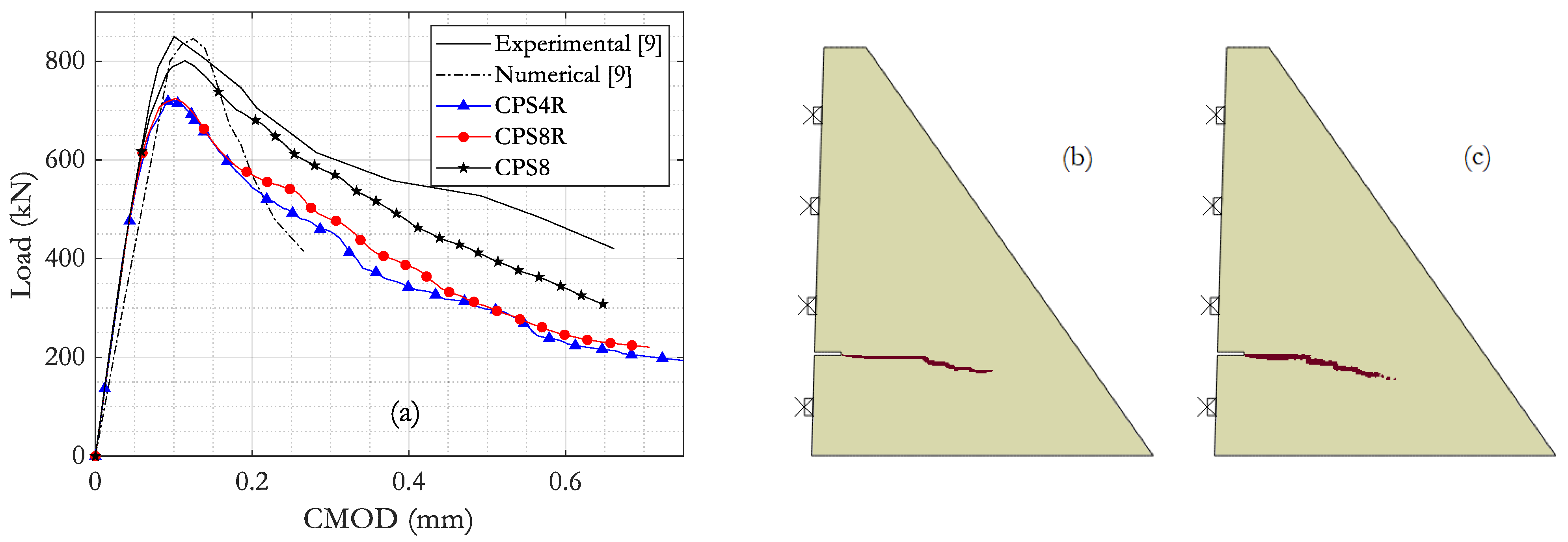
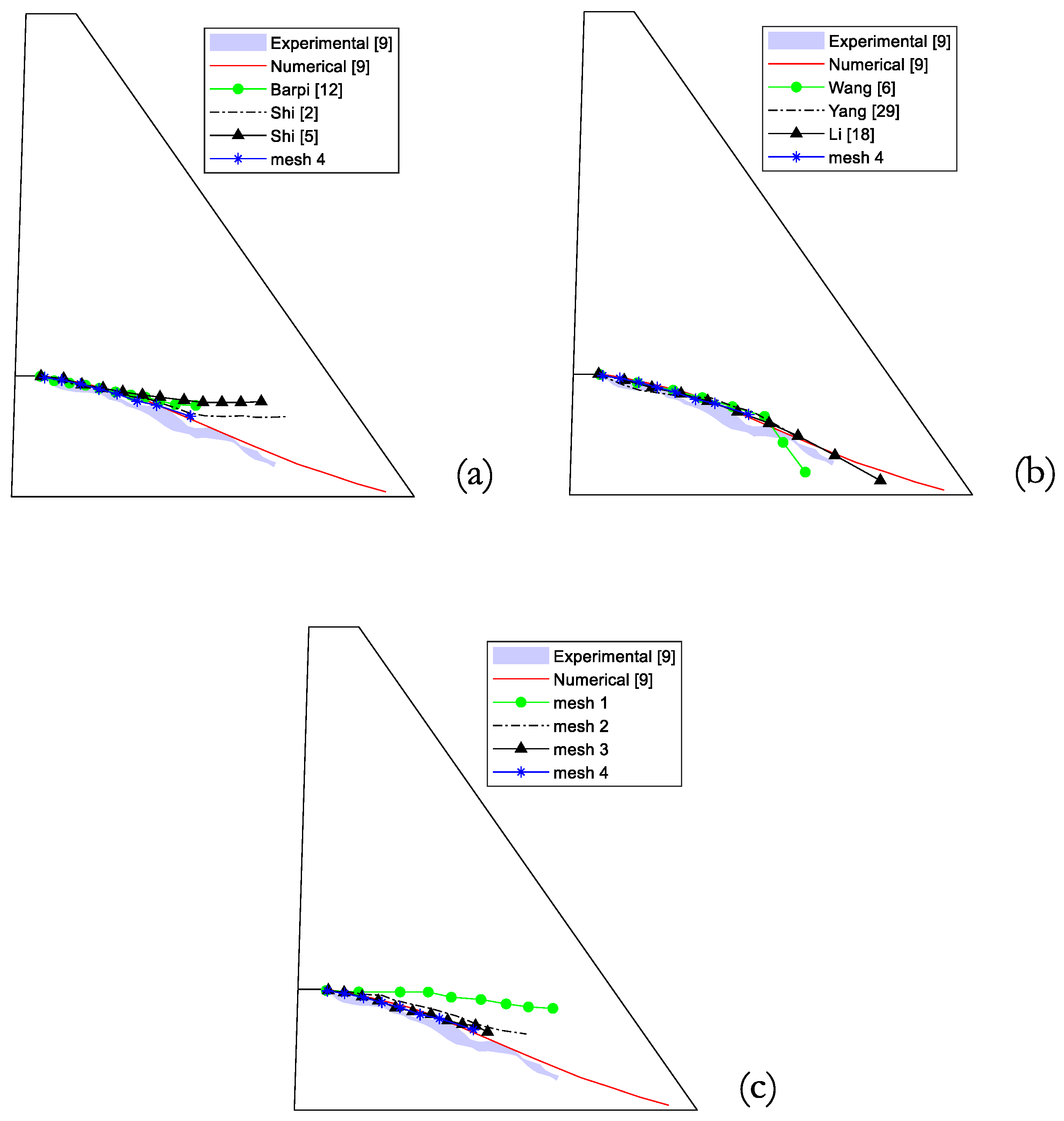
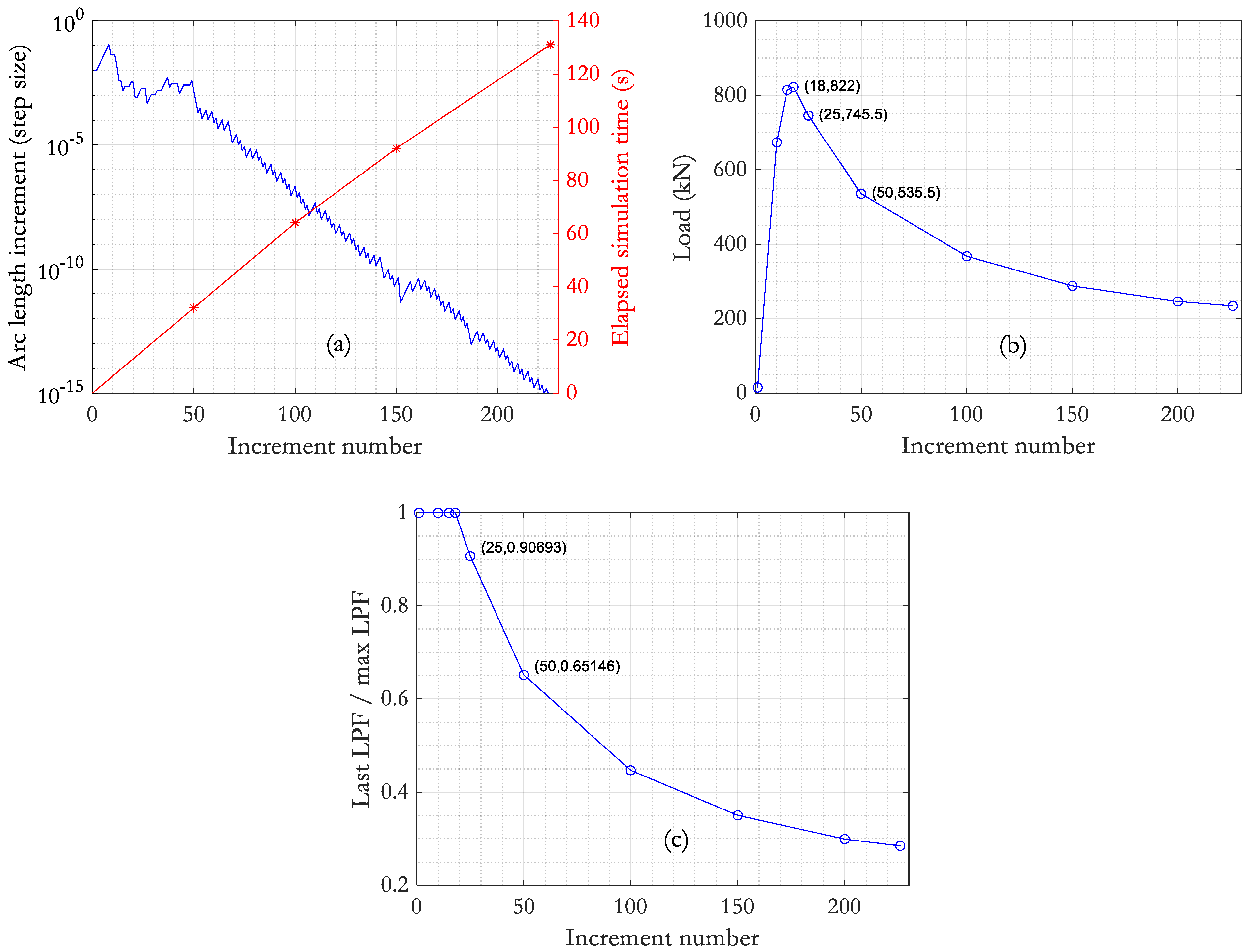
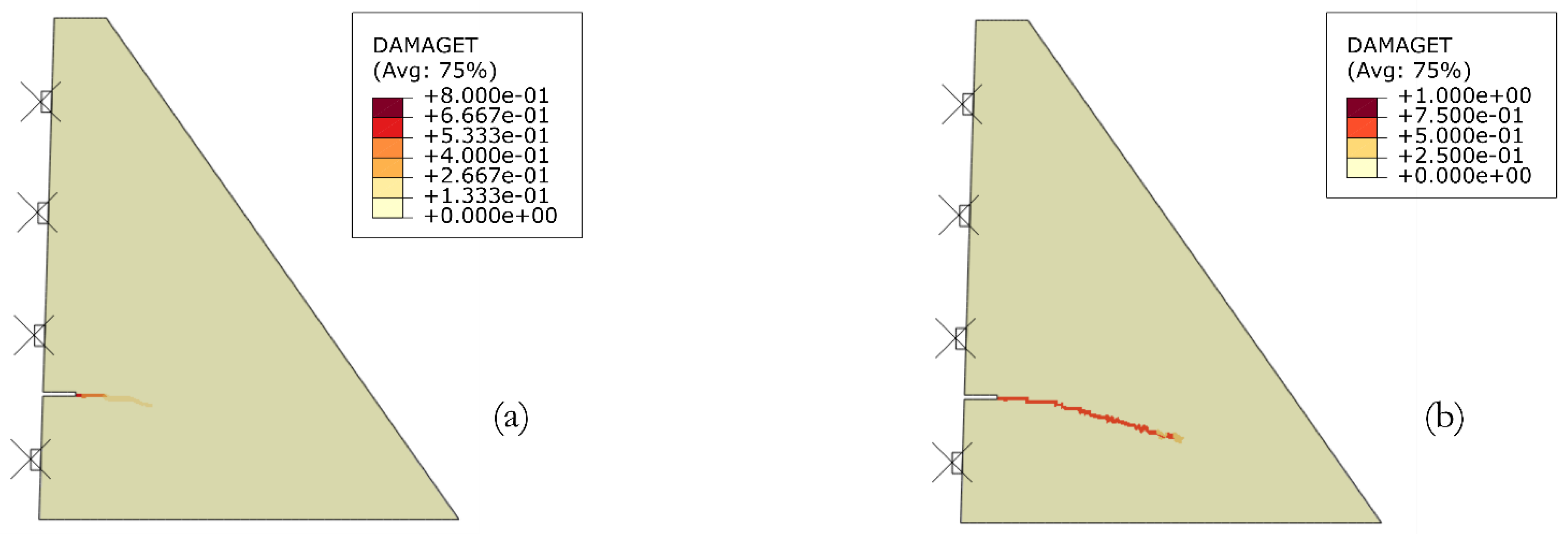
3.4. Simulation Results and Discussion

The results for the load-CMOD curves are presented in Figure 5 considering material models with linear and bilinear softening laws, as described in Section 3.2. These curves are also compared to Carpinteri et al.’s [9] experimental and numerical data. An expressive difference occurs between the peak loads provided by the linear softening model when compared to the reference results, with the exception of mesh 1. However, further refinement of the notch region (as shown for the more refined meshes) provides a convergence behavior for the peak load, which is 18% greater than the reference experimental value. This inconsistency is overcome with the use of the bilinear softening models. Using Rokugo et al.’s [31] softening curve, this difference is reduced to 4%, with the finite element models predicting a marginally lower peak load. Results provided by meshes 3 and 4 are almost identical, with negligible differences for a practical scope. An upper-bound result is achieved with the use of the fib model code 2010 [32] softening model. In this case, the peak load is 3% greater than the reference value. For the linear and bilinear models, the post-peak results are positioned between the experimental and numerical data provided by Carpinteri et al. [9], which is a common behavior for all the analyzed meshes. Results for mesh 1 using Rokugo et al.’s [31] bilinear softening are not available, because convergence was not achieved using this model. Conversely, results for this mesh are available using the fib model code 2010 [32], with a peak load that is 15% inferior to the reference results. When the bilinear models are compared, the softening curve provided by the fib model code 2010 [32] produces a more reliable approximation of the numerical results presented by Carpinteri et al. [9], specially at the first stages of the descending portion of the load-CMOD curve. Thereafter a convergence pattern is observed.
Further analyses are presented for comparison of the finite element results with the data retrieved in the literature survey. For the current observations, only the results for mesh 4 with bilinear softening model provided by fib model code 2010 [32] are selected. This analysis is depicted in Figure 6. The current results follow a similar pattern to Wang et al. [6]. Conversely, most past research data indicates a numerical behavior that follows Carpinteri et al.’s [9] numerical curve. Common aspects between the current simulations and past research include: (i) identical initial elastic behavior; and (ii) similar peak load values, with relative differences in the range of 10% when compared to the reference results.
An investigation is also performed for the analysis of crack trajectories. These results are presented in Figure 7, where the crack path is defined in terms of the concrete tensile damage variable (DAMAGET). For the sake of simplicity, these plots consider only two contour intervals, with the maximum threshold value set to 1 and using the default option of average element output at the nodes.
The level of refinement in the vicinity of the notch directly affects the trajectory behavior. For mesh 1, a refinement bias is noticeable, with crack trajectories following a horizontal path. For mesh 2, the first stages of cracking are mostly horizontal, aligned with the notch. Studies including further refinement, as those provided by meshes 3 and 4, lead to a 20 degrees path, without the delayed behavior presented by mesh 2. These analyses enable a better comprehension of the motivation behind the progressive refinement provided by mesh 4, which is effective in the representation of the crack trajectory and the load-CMOD curve, while using an inferior number of elements when compared to mesh 3.
Further studies are performed with the use of quadratic quadrilateral elements of types CPS8 and CPS8R, corresponding to full and reduced integration, respectively. For this investigation the original CPS4R elements of mesh 1 are replaced by CPS8 or CPS8R. These results are presented in Figure 8 and indicate that mesh bias can be circumvented to a certain extent with the use of higher-order elements using full integration. Load-CMOD results using CPS8 elements are in better agreement with Carpinteri et al.’s [9] numerical results, with the numerical model predicting a peak load that is only 6% inferior to the reference value. Results using CPS8R elements present just minor differences when compared to the CPS4R solution and follow the same limitations of the latter, indicating that reduced integration presents deficient performance for this analysis. The initial part of the crack trajectory is mostly horizontal and remains independent of the element choice. Despite that, slightly better behavior is perceived with a final 20 degrees-oriented segment, which was not observed using the original CPS4R elements.
A comparison of the mesh 4 results with crack trajectories recovered from past research is depicted in Figure 9. In parts “a” and “b”, a set of past results is juxtaposed to the experimental and numerical data presented by Carpinteri et al. [9], alongside with the results for mesh 4 using lower-order CPS4R with the fib model code 2010 [32] bilinear softening model. An initial agreement is verified for the first stages of crack propagation, regardless of the survey data source. However, a noticeable divergence is observed for the last stages, with Shi et al. [2] and Shi et al. [5] following a horizontal direction, while Wang et al. [6] and Yang et al. [29] trajectories are inclined toward the lower portion of the dam. The simulation results presented in this paper are in line with the latter. In a view of the load-CMOD curve results (shown in Figure 6), it can be seen that the apparent agreement of these curves with the reference data is not a guarantee that crack trajectories will follow a single expected behavior. Therefore, caution is advised when predicting reliable crack propagation using only load-CMOD results. Part “c” presents the results achieved in the current simulation using different refinement levels. Except for mesh 1, no expressive difference is perceived by means of a higher element concentration at the notch strip region. These results are satisfactory when compared to reference data provide by Carpinteri et al. [9].
Finally, performance information for processing each of the refinement levels, measured using the wallclock time available at the *.msg file is provided in Table 9. This information shows the total simulation time that elapsed while running Abaqus using the default job parameters which include the absence of CPU and GPGPU parallelization, and single nodal output precision. The current simulation results are based on a computational setup using an Intel® Core i7 1185G7 processor, with 32 GB DDR4 ram, 1TB NVMe SSD (maximum read transfer rate, 2100 MB/s, maximum write transfer rate, 1700 MB/s), running Windows 10 Pro. Furthermore, simulation data is limited to the numerical models using the fib model code 2010 [32] softening curve. The results indicate a progressive increment of processing time following the refinement level. Conversely, mesh 4 results are inferior to mesh 3. This leads to the conclusion that an adequate refinement, with a higher element concentration at the vicinity of the notch, enables an optimal use of computational resources, while producing results of the same quality as mesh 3. For this specific case with a wallclock time there is a reduction of 20%.
A more detailed analysis of the processing time of mesh 2 is possible from the evaluation of a combined plot where the increment of the arc length required for convergence is juxtaposed with the elapsed time for a given number of simulation increments (Figure 10a). These values were retrieved using the Abaqus *.msg file analyzer developed by Osterwisch [37]. In practical terms, this figure allows the identification of the minimum convergence criterion (step size) for a given increment, as well as the respective processing time. This analysis is even more interesting when associated with the horizontal load related to a given increment (Figure 10b). Additional information is also given with an analysis of the Load Pass Factor (LPF), as shown in Figure 10c. In Abaqus, the LPF is defined as the ratio between the load applied at the current increment and the load prescribed at the start of the analysis. Computations for the vertical axis of Figure 10c consider the ratio between the current value of the LPF and the maximum observed value of this variable in the previous increments. Due to the ascending nature of the LPF, this ratio is always equal to one until the peak load is achieved (which is computed automatically).
Finally, the results for the crack trajectories for increments 47 and 190 are presented (Figure 11). This set of images indicate that an abbreviated, but still satisfactory cracking response can be obtained in inferior time than that shown in Table 8. This occurs both for the load-CMOD curve and for the crack trajectory.
It is evident that some sort of criteria need to be defined for the total number of increments to be simulated. In this case, a Python script was developed, where an OS shell communication is established with the Abaqus executable and the *.sta file read at certain time intervals (as shown in Algorithm 1). This reading allows the calculation of the ratio shown in Figure 10c. The script interrupts the analysis at a certain threshold ratio prescribed by the user. For the results of Figure 11a a target ratio of 0.70 was used (and communication delay leads to a slightly inferior ratio, 0.68). This strategy enables the interruption of the analysis using a criterion which is not native to Abaqus and allows a practical analysis in inferior time than would be obtained with the criterion of the minimum arc-length size adopted in previous simulations (1 × 10⁻¹⁵), which leads to 226 increments (and a processing time of 131 s). The control through minimum arc-length size, although common is, in the authors’ opinion, less attractive than the restriction to a certain load ratio, which has the advantage of being a number with physical meaning for engineers. Obviously, the choice of this ratio influences both the load-CMOD curve and the crack trajectory. Once this value is established, analyses can be performed avoiding excessive computational costs. For the current simulation, the processing time was only 20 s, advancing to 47 increments, and the results allow an acceptable observation of the onset of crack propagation.
Algorithm 1. Python script that establishes OS shell communication with Abaqus and terminates the analysis if a prescribed load ratio is achieved.
“““
Python script that executes Abaqus and terminates the analysis if a prescribed ratio of the current load and the peak load is achieved. This enables the following features:
1. Interruption of the analysis for the peak load (ratio = 1);
2. or for a given user-defined ratio (ratio < 1).
MS-Windows versionos, numpy and time libraries are required
“““
import os
import numpy
import time
os.chdir(‘C:\\Users\\Polytechnique\\...)
jobname = ‘job-1’
os.system(‘abaqus job = ‘+jobname)
# desired target ratio of last LPF and max LPF
target = 0.70
# number of read file verifications
nreads = 12
# flag that indicates if target is achieved
flag = False
# result output function
def output(flag,count,jobname):
if flag:
txt = ‘ ‘
else:
txt = ‘ not ‘
print()
print(‘--------------------------------’)
print(‘ analysis summary ‘)
print(‘--------------------------------’)
print(‘# target rate’ + txt +’achieved after ‘ + str(count) + ’ verifications’)
print(‘# job terminated’)
os.system(‘abaqus terminate job = ‘+jobname)
sta_file.close()
# read file verifications (main code)
time.sleep(10) # 10s delay before first file reading
for count in list(numpy.arange(1.0,nreads + 1,1.0)):
time.sleep(5) # at 5s interval
print(‘----------------------------------’)
print(‘ verification # ‘+ str(count))
print(‘----------------------------------’)
# opens the *.sta file
sta_file = open(jobname + ’.sta’, ‘r’)
# reads the LPF columns of the *.sta file using numpy
LPF = numpy.loadtxt(sta_file,usecols = (6),skiprows = 5)
print()
print(‘LPF vector’)
print(LPF)
# computes the ratio
ratio = LPF[−1]/max(LPF)
print()
print(‘ratio of last LPF and max LPF: ‘, str(ratio))
if ratio <= target:
flag = True
sta_file.close()
break
else:
print()
print(‘# target rate not achieved’)
print()
# output function call
output(flag,count,jobname)

4. Concluding Remarks

This paper discussed the main aspects of the modeling and simulation of a concrete gravity dam cracking response based on a broad literature survey. The material and numerical models have evolved over the years. Nevertheless, classical benchmarks remain reliable references for the performance analysis of this progress. The best practices of modeling, simulation, verification, and validation were presented. Carpinteri et al.’s [9] pre-notched dam was selected to demonstrate the authors’ recommendations. A finite element model was defined using Abaqus for a series of refinement levels, including the use of linear and bilinear tensile softening models, as well as an investigation of higher-order elements with full and reduced integration. Final investigations, including a Python script, were also presented for the optimal analysis of the nonlinear model. The following key observations emerged from the current study:
  • The steps involved in modeling concrete gravity dam cracking are not obvious. A linear elastic simulation is achievable for any engineer who has some familiarity with commercial finite element software. However, the learning curve is considerable for adequate representation of the nonlinear concrete behavior. This is due to the requirement of multiple parameters that exert direct influence on the nonlinear response; such as element type, mesh refinement, material properties, solver options, proper boundary conditions, and finally, the proper comprehension of the scope and limitations of a nonlinear analysis.
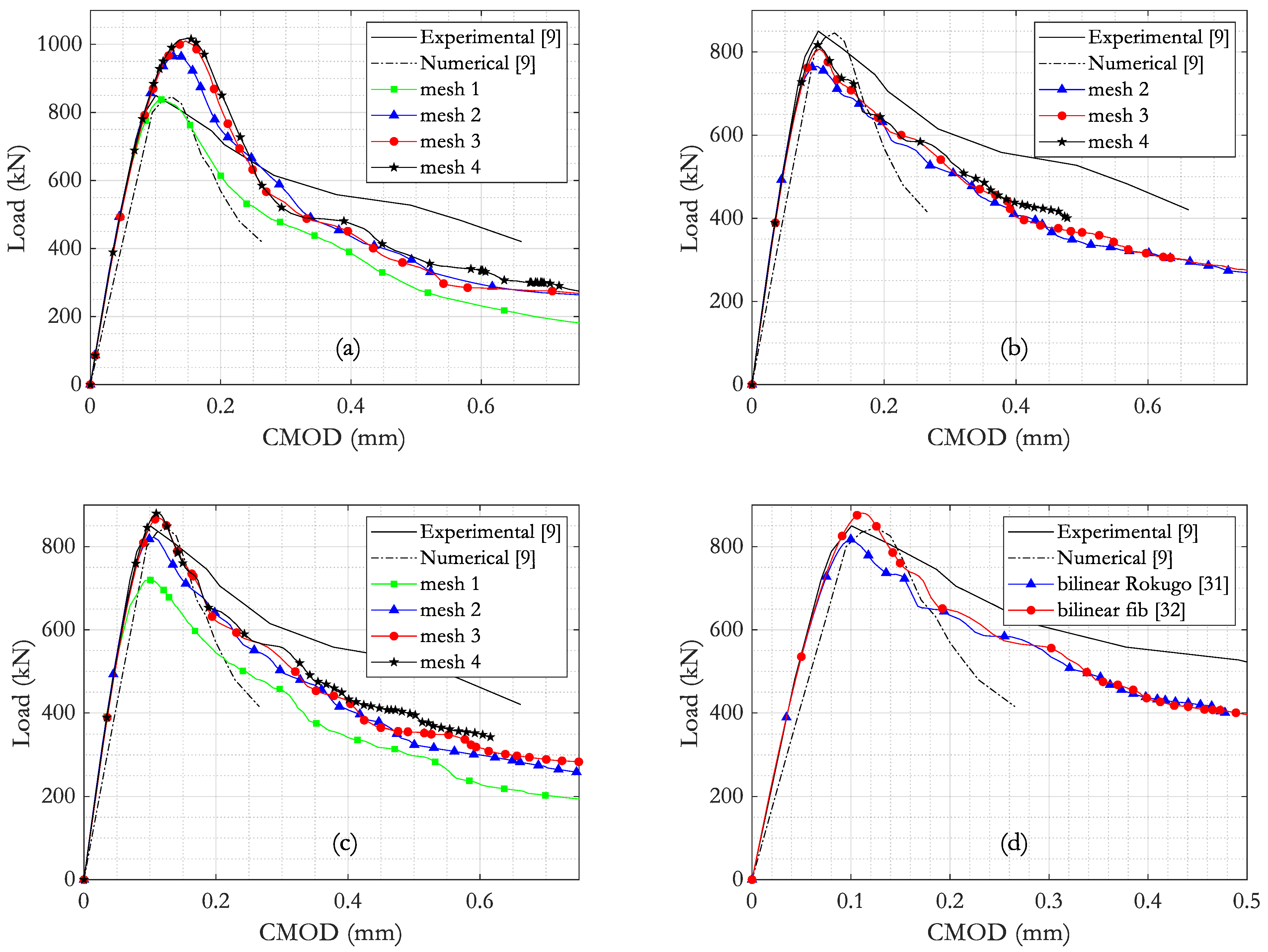
  • For the selected benchmark, a linear softening model overestimates the load-CMOD curve, and a bilinear softening model provides a better estimate, with an accurate prediction of the peak load value.
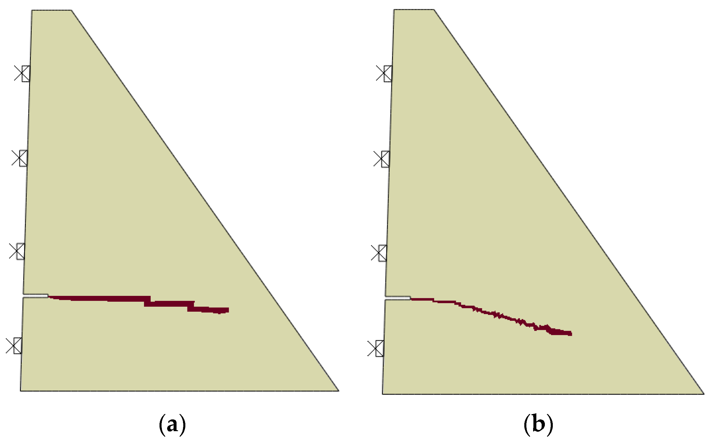
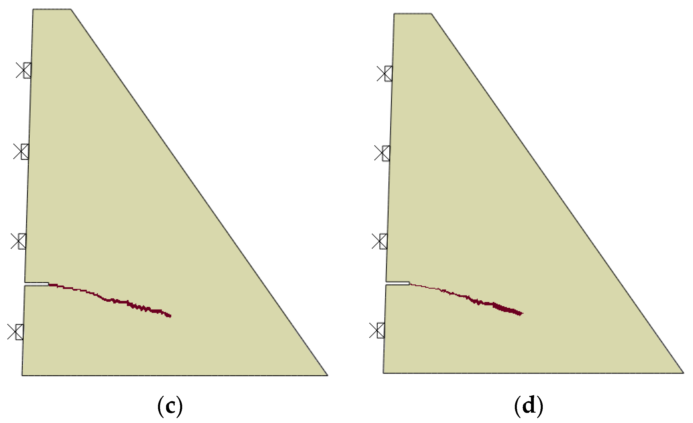
  • The apparent agreement between load-CMOD curves is not converted to similar crack trajectories. Results provided by the coarser mesh using the fib model code 2010 [32] diverge from the expected numerical and experimental data. In this case, a horizontal path is observed. The remaining meshes present a mostly 20 degrees orientation that follows the reference data.
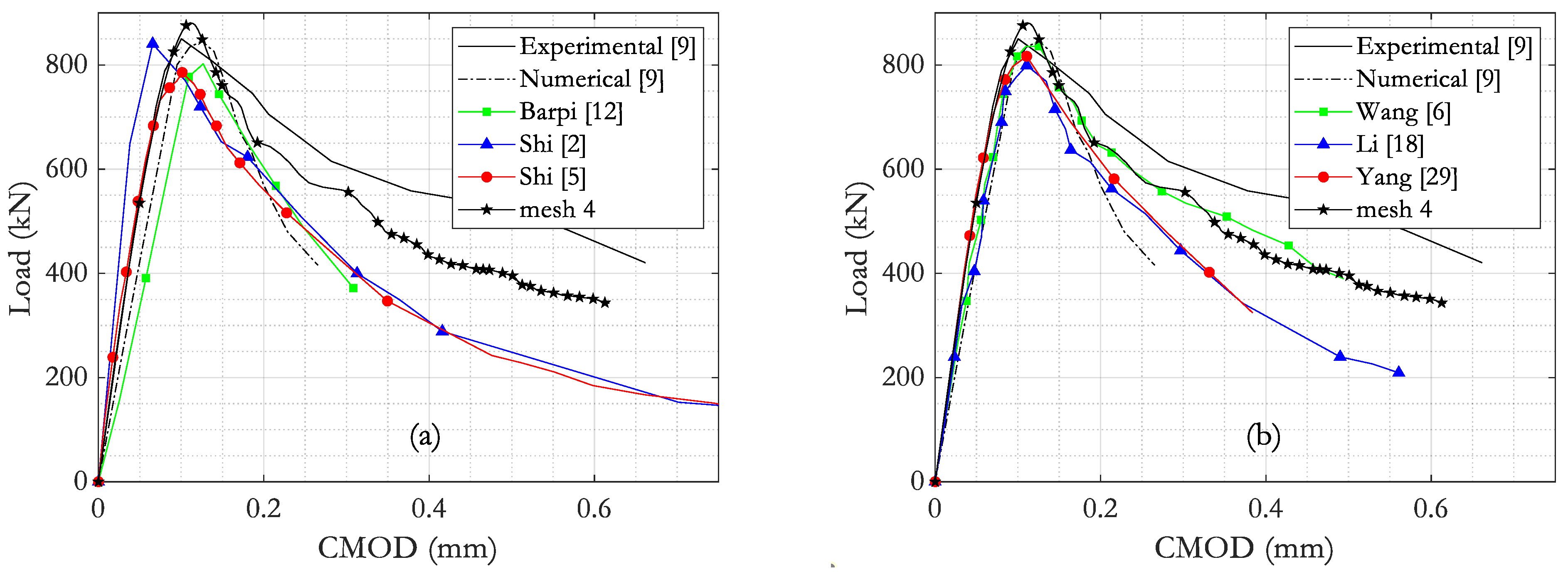
  • Distinct cracking behavior is observed when the literature survey results are analyzed. However, crack trajectories are similar for at least the first 40% of the predicted crack length, regardless of the data source.
  • There is only a marginal gain with refinements advancing from mesh 2 toward mesh 4, as this can be observed in both load-CMOD and crack trajectory results. Therefore, the refinement with an element edge size of approximately 15 mm along the notch strip region provides satisfactory results, with a processing time of about 2 min.
  • The use of computational resources in an efficient manner is always desirable for the solution of nonlinear problems. Consequently, good judgment is expected in the need for mesh refinement at regions where crack propagation is likely to occur. The temptation of a uniform refinement at the notch strip region should be avoided, as this leads to inefficient computations.
  • The proposed Python script emerges as a valuable tool for time-demanding analyses in Abaqus, enabling solution control for a given target ratio, and avoiding computation of load increments that are beyond the practical engineer’s expectations, while still providing meaningful results.

Author Contributions

Conceptualization, P.L.; methodology, P.L.; software, P.M.V.R.; validation, P.L. and P.M.V.R.; formal analysis, P.M.V.R.; investigation, P.M.V.R.; resources, P.L.; writing—original draft preparation, P.L. and P.M.V.R.; writing—review and editing, P.L. and P.M.V.R.; supervision, P.L.; project administration, P.L.; funding acquisition, P.L. and P.M.V.R. All authors have read and agreed to the published version of the manuscript.

Funding

This research was funded by the Brazilian National Council for Scientific and Technological Development (CNPq), grant number 200223/2021-6 and the Natural Sciences and Engineering Research Council of Canada, with provision of the APC charges and software licenses.

Conflicts of Interest

The authors declare no conflict of interest. The funders had no role in the design of the study; in the collection, analyses or interpretation of data; in the writing of the manuscript; or in the decision to publish the results.

References

  1. Bhattacharjee, S.S.; Léger, P. Application of NLFM models to predict cracking in concrete gravity dams. J. Struct. Eng. 1994, 120, 1255–1271. [Google Scholar] [CrossRef]
  2. Shi, Z.; Suzuki, M.; Nakano, M. Numerical analysis of multiple discrete cracks in concrete dams using Extended Fictitious Crack Model. J. Struct. Eng. 2003, 129, 324–336. [Google Scholar] [CrossRef]
  3. Mirzabozorg, H.; Ghaemian, M. Non-linear behavior of mass concrete in three-dimensional problems using a smeared crack approach. Earthq. Eng. Struct. Dyn. 2005, 34, 247–269. [Google Scholar] [CrossRef]
  4. Hariri-Ardebili, M.A.; Seyed-Kolbadi, S.M.; Mirzabozorg, H. A smeared crack model for seismic failure analysis of concrete gravity dams considering fracture energy effects. Struct. Eng. Mech. 2013, 48, 17–39. [Google Scholar] [CrossRef]
  5. Shi, M.; Zhong, H.; Ooi, E.T.; Zhang, C.; Song, C. Modelling of crack propagation of gravity dams by scaled boundary polygons and cohesive crack model. Int. J. Fract. 2013, 183, 29–48. [Google Scholar] [CrossRef]
  6. Wang, G.; Lu, W.; Zhou, C.; Zhou, W. The influence of initial cracks on the crack propagation process of concrete gravity dam-reservoir-foundation systems. J. Earthq. Eng. 2015, 19, 991–1011. [Google Scholar] [CrossRef]
  7. Dias, I.F.; Oliver, J.; Lemos, J.V.; Lloberas-Valls, O. Modeling tensile crack propagation in concrete gravity dams via crack-path-field and strain injection techniques. Eng. Fract. Mech. 2016, 154, 288–310. [Google Scholar] [CrossRef]
  8. Yao, F.; Yang, Z.J.; Hu, Y.J. An SBFEM-Based model for hydraulic fracturing in quasi-brittle materials. Acta Mech. Solida Sin. 2018, 31, 416–432. [Google Scholar] [CrossRef]
  9. Carpinteri, A.; Valente, S.; Ferrara, G.; Imperato, L. Experimental and numerical fracture modelling of a gravity dam. In Fracture Mechanics of Concrete Structures, 1st ed.; Science, E.A., Ed.; CRC Press: London, UK, 1992; pp. 351–360. [Google Scholar]
  10. Valente, S.; Barpi, F. On singular points in mixed-mode cohesive crack propagation. Trans. Eng. Sci. 1994, 6, 167–174. [Google Scholar]
  11. Barpi, F. Modelli Numerici Per lo Studio dei Fenomeni Fessurativi Nelle Dighe. Ph.D. Thesis, Politecnico di Torino, Torino, Italy, 1996. (In italian). [Google Scholar]
  12. Barpi, F.; Valente, S. Numerical simulation of prenotched gravity dam models. J. Eng. Mech. 2000, 126, 611–619. [Google Scholar] [CrossRef]
  13. Carpinteri, A.; Cornetti, P.; Barpi, F.; Valente, S. Cohesive crack model description of ductile to brittle size-scale transition: Dimensional analysis vs. renormalization group theory. Eng. Fract. Mech. 2003, 70, 1809–1839. [Google Scholar] [CrossRef]
  14. Ghrib, F.; Tinawi, R. Nonlinear behavior of concrete dams using damage mechanics. J. Eng. Mech. 1995, 121, 513–527. [Google Scholar] [CrossRef]
  15. Cai, Q. Finite Element Modelling of Cracking in Concrete Gravity Dams. Ph.D. Thesis, University of Pretoria, Pretoria, South Africa, 2007. [Google Scholar]
  16. Durieux, J.; van Rensburg, B. Development of a practical methodology for the analysis of gravity dams using the non-linear finite element method. J. S. Afr. Inst. Civ. Eng. 2016, 58, 1–13. [Google Scholar] [CrossRef]
  17. Chahrour, A.H.; Ohtsu, M. Simulation of discrete cracking in a concrete gravity dam. Concr. Eng. Annu. Proc. 1994, 16, 45–50. [Google Scholar]
  18. Li, J.-b.; Gao, X.; Fu, X.-a.; Wu, C.; Lin, G. A nonlinear crack model for concrete structure based on an Extended Scaled Boundary Finite Element Method. Appl. Sci. 2018, 8, 1067. [Google Scholar] [CrossRef]
  19. Oberkampf, W.L.; Roy, C.J. Verification and Validation in Scientific Computing; Cambridge University Press: New York, NY, USA, 2010. [Google Scholar]
  20. Roache, P.J. Verification and Validation in Computational Science and Engineering; Hermosa Publishers: Albuquerque, NM, USA, 1998. [Google Scholar]
  21. Shi, Z. Numerical analysis of mixed-mode fracture in concrete using extended fictitious crack model. J. Struct. Eng. 2004, 130, 1738–1747. [Google Scholar] [CrossRef]
  22. Lohrasbi, A.R.; Attarnejad, R. Crack growth in concrete gravity dams based on discrete crack method. Am. J. Eng. Appl. Sci. 2008, 1, 318–323. [Google Scholar] [CrossRef]
  23. Wu, Z.; Rong, H.; Zheng, J.; Dong, W. Numerical method for mixed-mode I–II crack propagation in concrete. J. Eng. Mech. 2013, 139, 1530–1538. [Google Scholar] [CrossRef]
  24. Oliver, J.; Huespe, A.E.; Pulido MD, G.; Chaves, E. From continuum mechanics to fracture mechanics: The Strong Discontinuity Approach. Eng. Fract. Mech. 2002, 69, 113–136. [Google Scholar] [CrossRef]
  25. Roth, S.-N.; Léger, P.; Soulaïmani, A. A combined XFEM–damage mechanics approach for concrete crack propagation. Comput. Methods Appl. Mech. Eng. 2015, 283, 923–955. [Google Scholar] [CrossRef]
  26. Sha, S.; Zhang, G. Modeling of hydraulic fracture of concrete gravity dams by Stress-Seepage-Damage Coupling Model. Math. Probl. Eng. 2017, 2017, 8523213. [Google Scholar] [CrossRef]
  27. Attard, M.M.; Tin-Loi, F. Numerical simulation of quasibrittle fracture in concrete. Eng. Fract. Mech. 2005, 72, 387–411. [Google Scholar] [CrossRef]
  28. Su, K.; Zhou, X.; Tang, X.; Xu, X.; Liu, Q. Mechanism of cracking in dams using a Hybrid FE-Meshfree Method. Int. J. Geomech. 2017, 17. [Google Scholar] [CrossRef]
  29. Yang, D.; He, X.; Yi, S.; Liu, X. An improved ordinary state-based peridynamic model for cohesive crack growth in quasi-brittle materials. Int. J. Mech. Sci. 2019, 153-154, 402–415. [Google Scholar] [CrossRef]
  30. Dassault Systèmes. Abaqus CAE (Version 6.14-1) [Computer Software]. 2014. Available online: https://www.3ds.com/products-services/simulia/products/abaqus/abaquscae/ (accessed on 7 December 2022).
  31. Rokugo, K.; Iwasa, M.; Suzuki, T.; Koyanagi, W. Testing methods to determine tensile strain softening curve and fracture energy of concrete. In Fracture Toughness and Fracture Energy-Test Method for Concrete and Rock; Mihashi, H., Takahashi, H., Wittmann, F.H., Eds.; Balkema: Rotterdam, The Netherlands, 1989; pp. 153–163. [Google Scholar]
  32. Fédération Internationale du Béton—Fib. Fib Model Code for Concrete Structures 2010; Ernst & Sohn: Berlin, Germany, 2013. [Google Scholar]
  33. Lubliner, J.; Oliver, J.; Oller, S.; Oñate, E. A plastic-damage model for concrete. Int. J. Solids Struct. 1989, 25, 299–326. [Google Scholar] [CrossRef]
  34. Lee, J.; Fenves, G.L. Plastic-damage model for cyclic loading of concrete structures. J. Eng. Mech. 1998, 124, 892–900. [Google Scholar] [CrossRef]
  35. Lee, J.; Fenves, G.L. A plastic-damage concrete model for earthquake analysis of dams. Earthq. Eng. Struct. Dyn. 1998, 27, 937–956. [Google Scholar] [CrossRef]
  36. Wosatko, A.; Winnicki, A.; Polak, M.A.; Pamin, J. Role of dilatancy angle in plasticity-based models of concrete. Arch. Civ. Mech. Eng. 2019, 19, 1268–1283. [Google Scholar] [CrossRef]
  37. Osterwisch, C. Abaqus Msg File Buddy. Available online: https://msgfile.info/ (accessed on 7 December 2022).
Figure 1. Experimental test performed in a 1:40 scaled-down model. From: Fracture Mechanics of Concrete Structures: Proceedings, Carpinteri et al. [9], Copyright ©1992 and Imprint. Reproduced by permission of Taylor & Francis Group.
Infrastructures 08 00050 g001
Figure 2. Geometry, boundary conditions, coordinates, and details for the finite element simulation (units: mm).
Infrastructures 08 00050 g002
Figure 3. Different stress-crack representations for the adopted tension softening models: (a) linear, (b) bilinear provided by fib model code 2010 [32], (c) bilinear based on Rokugo et al. [31].
Infrastructures 08 00050 g003
Figure 4. Different levels of refinement applied for the finite element modeling: (a) mesh 1, (b) mesh 2, (c) mesh 3, (d) mesh 4. Dimensions: mm.
Infrastructures 08 00050 g004
Figure 5. Load versus CMOD results for: (a) linear softening; bilinear softening using (b) Rokugo et al. [31] and (c) fib model code 2010 [32]; (d) comparison of bilinear model results for mesh 4.
Infrastructures 08 00050 g005
Figure 6. Load versus CMOD curves retrieved in the literature survey from: (a) data from 2000 to 2013, (b) data from 2015 to 2019; and comparison with the results for mesh 4 using the bilinear softening model provided by fib model code 2010 [32].
Infrastructures 08 00050 g006
Figure 7. Crack trajectories for different refinement levels using fib model code 2010 [32] bilinear softening model: (a) mesh 1, (b) mesh 2, (c) mesh 3, (d) mesh 4.
Infrastructures 08 00050 g007aInfrastructures 08 00050 g007b
Figure 8. (a) Load-CMOD curve for mesh 1 using linear and quadratic finite elements, and the corresponding crack trajectory for the higher-order mesh using (b) CPS8R and (c) CPS8 elements.
Infrastructures 08 00050 g008
Figure 9. Crack trajectories recovered from past research (a,b) and comparison with mesh 4 results; (c) evolution of crack trajectories in the current simulation using different refinement levels.
Infrastructures 08 00050 g009
Figure 10. Combined results for mesh 02 including: (a) convergence requirements and elapsed simulation time; (b) horizontal load for a given increment number; and (c) ratio of the LPF of the current increment and the highest LPF simulation value observed in the previous increments.
Infrastructures 08 00050 g010
Figure 11. Crack trajectories for mesh 02 considering the following increments: (a) 47, (b) 190.
Infrastructures 08 00050 g011
Table 1. Description of experimental models analyzed by Carpinteri et al. [9].
Test CaseDescription
1Notch-depth ratio = 0.1; this simulation was stopped at peak load, as a result of a failure at the weakest section of the dam foundation. Combined vertical and horizontal loads were considered.
2Notch-depth ratio = 0.1; this simulation is a continuation of Test Case 1 model, which was reinitiated after the reinforcement of the previous failure region. Self-weight loads were removed from this case.
3Notch-depth ratio = 0.2; this simulation considers only horizontal loads provided by the actuators.
Table 2. Benchmark information availability considering finite elements with discrete crack models.
SourceTest CaseLoad-CMODCrack Trajectories
Valente and Barpi [10]2
Barpi [11]; Barpi and Valente [12]; Shi et al. [2]; Wu et al. [23]2, 3
Shi [21]3
Lohrasbi and Attarnejad [22]2
Table 3. Benchmark information considering smeared crack and enhanced finite elements.
SourceTest CaseLoad-CMODCrack Trajectories
Bhattacharjee and Léger [1]; Ghrib and Tinawi [14]; Oliver et al. [24]; Mirzabozorg and Ghaemian [3]; Cai [15]; Hariri-Ardebili et al. [4]; Roth et al. [25]; Wang et al. [6]; Durieux and Rensburg [16]; Sha and Zang [26]3
Dias et al. [7]2
Table 4. Benchmark information availability considering conventional and enhanced boundary elements.
SourceTest CaseLoad-CMODCrack Trajectories
Chahrour and Ohtsu [17]; Shi et al. [5]; Yao et al. [8]; Li et al. [18]2
Table 5. Benchmark information considering particle or meshfree methods.
SourceTest CaseLoad-CMODCrack Trajectories
Attard and Tin-Loi [27]3
Su et al. [28]2, 3
Yang et al. [29]2
Table 6. Concrete material properties.
E (Gpa)vft (MPa)Gf (N/mm)
35.700.103.600.184
Table 7. Plasticity parameters adopted in Abaqus for the numerical models.
ψεσb0/σc0KcViscosity Parameter
4000.101.200.670
Table 8. Solver parameters for the arc-length method.
ParameterValue
Initial increment0.01
Minimum increment1 × 10−15
Maximum increment0.2
Table 9. Performance information in terms of wallclock time for the different refinement levels using the fib model code 2010 [32] softening curve.
Mesh1234
Wallclock time (s)91131290232
Disclaimer/Publisher’s Note: The statements, opinions and data contained in all publications are solely those of the individual author(s) and contributor(s) and not of MDPI and/or the editor(s). MDPI and/or the editor(s) disclaim responsibility for any injury to people or property resulting from any ideas, methods, instructions or products referred to in the content.

