Shaking Table Design for Testing Earthquake Early Warning Systems

Abstract

The unpredictability in time of seismic activities and the dependence of tectonic movements on a multitude of factors challenges specialists to identify the most accurate related methods to avoid catastrophes associated with hazards. Early warning systems are critical in reducing negative effects in the case of an earthquake with a magnitude above 5 MW. Their precision is all the better as they corroborate and transmit more information collected from the regional or on-site sensory nodes to a central unit that discloses events and estimates the epicentral location, earthquake magnitude, or ground shaking amplitude. The shaking table is the proper instrument for evaluating an early warning systems’ dynamic response and performance under specific vibration conditions. To this issue, the paper presents a laboratory single-axis shaking table with a small-scale, low-cost design and an accurate displacement control. Experiments based on a suite of 12 real earthquakes provided results with very small errors related to similar models, bearing out the designed shaking table is suitable for early earthquake warning system response testing for high magnitude earthquakes.

1. Introduction

An earthquake generates a succession of elastic waves that travel along and through the surface of the Earth, from the epicentral location to the recording seismic station. The first arrivals are P-waves (primary compressional waves involving volumetric disturbances) that produce ground motion along the direction of propagation [1]. Faster-moving P-waves trigger sensors that, in turn, transmit signals to the data processing centers. The secondary S-waves recorded (shear waves involving only interior deformation of homogeneous solids and no volume change) are 1.7 times slower than P-waves but have a higher destructive amplitude [2]. Ground motion-sensitive detection is based on the seismic wave’s velocity or acceleration, measured on the vertical axis of the propagation [3]. The seismic vibrations are recorded with sensitive instrumentation able to detect the transient oscillations within a moving reference frame, operating continuously and providing an accurate response related to the amplitude and frequency of the ground motion. Using this early-stage event detection, earthquake early warning systems (EEWS) can operate, through specific algorithms, to promptly estimate real-time information (epicenter, magnitude, intensity, and potential consequences of an earthquake), and send regional alarms a few seconds before the event occurs [4]. EEWSs of a regional type (point-source or finite fault) comprise a network of seismic sensors located at the expected epicentral zone or zone of high seismicity in a region and are intended to predict ground motion at sites located further away from the event. EEWSs of an on-site type comprise a limited set of seismic stations located at (for site-specific systems) or near (for front-detection systems) particular sites of interest. Each type has a major advantage: the regional EEWS transmits the specific earthquake data more precisely, and the on-site EEWS transmits warnings more quickly to vulnerable locations [5]. EEWS warnings are broadcast for seismic intensities greater than 4.5 MW because setting the alarm system below this threshold can generate false alarms and interrupt technological processes whose commissioning costs are high. The latest types of seismic warning systems operate based on convolutional neural networks, trained and validated for earthquakes with many strong motions. Their role is to select relevant features from P-waves to predict whether the peak ground acceleration of subsequent waves usually surpasses 80 cm/s²—a threshold acceleration value from which people strongly feel the ground motion [6]. As the time window is critical for EEWS triggering, these artificial methods for ground motion prediction require a period parameter from which to follow a reasonable leading time.

Due to the complexity of infrastructures and human activities, continuous and long-term monitoring of seismicity is indispensable. This assessment needs more than broadband precision sensors and new real-time transmission systems (such as recently discovered prompt elastogravity signals used to track earthquake growth instantaneously after the event reaches a certain magnitude [7]). A wide multisensor network approach is required to provide information for the complete characterization of the ground shaking, coupled with the detection of permanent surface deformation (GPS and satellite), soil gas emissions, and atmospheric anomalies, allowing us to extend the knowledge of the spectrum of observations associated with earthquakes. [8]. Particular attention in long-term seismic monitoring must be paid to background noise evaluation and quantification. This ambient noise, caused by natural causes (tides, storms, ocean infragravity waves, atmospheric pressure variations, and diurnal surface heating) or artificial causes (induced by human activities), produces continuous background motions called earth tremors or microseisms. Background motions are temporally and spatially variable. They vary with frequency and have infinite energy (but finite power), unlike earthquakes, which last a finite amount of time and have finite energy.

According to the field regulation, a structural model or a nonstructural component seismic certification is confirmed by attesting on a shaking table, following ICC-ES 156 procedures [9] and ASCE 7 Standard provisions. From small laboratory models to large process models, shaking tables are precision equipment that uses prototype scaling techniques to appraise the dynamic behavior of a structure, regardless of its size. As an example, the research of [10] details the achievement of the first shaking table for testing a 1/50 scale high-rise building model for the 101-storey Shanghai World Financial Center Tower to identify the dynamic characteristics, seismic responses, and weak positions under seldom-occurring earthquakes. In comparison, the Japanese National Research Institute for Earth Science and Disaster Resilience conducts full-scale or large-scale experiments on the world’s largest 3D shaking table driven by five horizontal actuators installed in each direction and by 14 vertical actuators (platform size: 20 × 15 m, 12,000 kN maximum loading capacity, which reaches a maximum acceleration of 9 m/s² on the X and Y axis and 15 m/s² on the Z axis) [11]. With regard to laboratory equipment, there are certified small-scale vibrating tables on a single axis or multiple axes up to six degrees of freedom—with a servomotor, hydraulic, or hybrid actuation. Electro-dynamic vibrating tables prevail in having the advantage of being able to be driven at high frequencies and to impose acceleration as an input excitation. They may be designed with different parameters, e.g., a maximum acceleration of 1.5 g, a maximum displacement of ±75 mm, and a platform dimension of 500 mm × 500 mm [12]; a maximum acceleration of 1 g, a maximum displacement of ±75 mm, and a platform dimension of 1500 mm × 2000 mm [13]; a maximum acceleration of 1.9 g, a maximum displacement of ±30 mm, and a platform dimension of 76 mm × 76 mm [14]. Regarding mass-produced vibrating tables, there are accessible, mid-size, open-architecture, single-axis shakers with a maximum acceleration of 2.5 g, a maximum displacement of ±76 mm, and a platform dimension of 460 mm × 460 mm [15]. A hydraulic-driven shaking table is described in [16], with a maximum acceleration of 4 g, a maximum displacement of ±76.2 mm, and a platform dimension of 915 mm × 915 mm. An electro-hydraulic shaking table imposes a force and/or torque as the input excitation and generally consists of servo-valves, hydraulic actuators, a motion table, a measurement system, and an accurate control system. It presents similar parameters: a maximum acceleration of 2 g, maximum displacement on three axes: ±100 mm, and a platform dimension of 1500 mm × 1500 mm [17]. High-fidelity tracking of a shaking table is an important research topic, being related to different control strategies for attaining real-time replication of the desired acceleration signal. The nonlinear characteristics of the shake table and the dynamics of the structure to be examined impair the shake table’s control. Vibrating tables are usually driven by a proportional–integration–derivative (PID) controller or similar methods, such as a three-variable controller [18]. Depending on the destination and the specifics of the structure or infrastructure, seismic performance is typically tested by dynamic analysis, in particular, modal response spectra analysis or seismic analysis based on static methods (linear or nonlinear time-history analyses) [19].

EEWS testing is less covered in the specialized literature, being considered a nonstructural component. Most of the tests conducted in this field aim to establish the seismic performance of a structure in order to guarantee the safety of people in particular premises and their vicinity and to ensure their operation in case of a hazard by calculating the structure’s response when subjected to earthquakes [20].

In order to assess the accuracy and limitations of a seismic sensor as a part of an EEWS, a low inertial uniaxial shaking table was designed to replicate real earthquake events in the laboratory. The shaking table was validated by testing its capability to correctly transfer the input reference seismic waveform. Its accuracy regarding the displacement response attested to the high-fidelity waveform replication.

2. Description of a Seismic Simulation Experiment Using Shaking Table

Given that the parameters that characterize the low-frequency content of strong ground motions are the mean period and the average spectral period, and the high-frequency content is characterized by the smoothed spectral predominant period [21], the shaking table for EEWS seismic sensors was tested following this scalar. The predominant spectral period does not adequately describe the frequency content of a strong ground motion and is not recommended.

As earthquake alert systems only use the vertical component of the seismic wave (herein input data) for disclosure, the seismic simulation was made on a single-axis shaking table. The system was electrodynamically powered, servo-controlled with a close loop PID, and operated with any type of computer-generated waveform, herein earthquake profiles. The servomotor-driven concept was chosen over the servo-hydraulic actuation because of its nonlinearity at high amplitude input signals or eventually due to control input saturation, directional change of valve opening, friction, and valve overlap. The experimental uniaxial vibrating table components were (Figure 1):

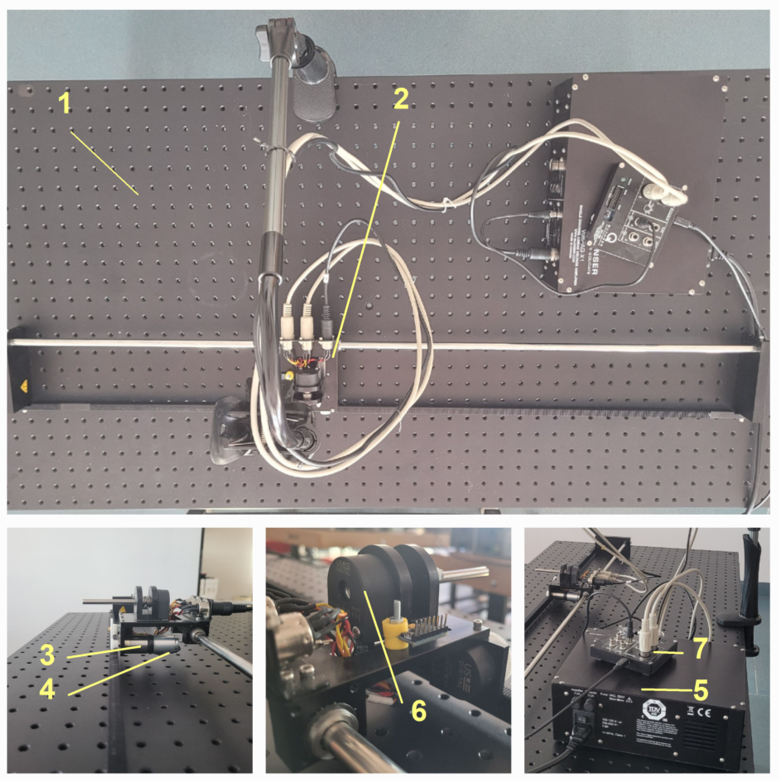
• A fixed steel frame/plate 1200 × 800 mm with mounting holes of Ø16 mm;
• Linear guiding axis 102 cm long, with a 10 × 14 × 9 cm aluminum cart for regular, continuous movement. The cart was driven by a rack and pinion mechanism of Ø6.35 mm and 24 teeth and slid along a stainless steel shaft using linear bearings. The cart weighed 500 g and allowed an extra mass of 370 g, achieving a maximum travel distance of 81.4 cm. Fulfilling the displacement carrying two masses ensures more inertia to absorb the structure’s vibrations.
• A DC servomotor with 4160 rpm and 40 × 10³ rad/s² angular acceleration for robust and precise actuation, back-EMF constant of 0.804 mV/rpm, a torque constant of 7.67 × 10⁻³ Nm/A, and a mechanical time constant of 17 ms.
• A gearbox (23/1 series with 1 stage, 100% efficiency, and 3.71:1 reduction ratio) for decreasing the load on the servomotor;
• A linear voltage-controlled power amplifier for supplying the brush DC micro motor with 6 V. The amplifier was supplied from the electricity grid with 230 V AC, allowing a continuous voltage output of ±24 V and a command of ±10 V.
• A high-resolution optical encoder for precise positioning: 0.0235 mm resolution (4096 counts per revolution in quadrature mode/1024 lines per revolution), tracking to 10,000 rpm. This served as a rotary to digital converter, using phased array detector technology. The position pinion had Ø148 mm and 56 teeth.
• An eight configurable digital inputs/output channels data acquisition board, connected to the encoder, which converts real-time shaft angle, speed, and direction into TTL-compatible quadrature outputs and is controlled through a PID loop in LabView. It had two 5-pin DIN Encoder Input connectors, through which it received 16-bit count values. The initial encoder count can be stated. The encoder can also be configured to reload the initial encoder count on an index pulse.

The proportional–integral–derivative controller is suitable for applications where continuously modulated control is required. A fine-tuned PID controller has parameters adapted to the dynamic performance of the process so that the control system becomes faster and more stable. If the process dynamics fluctuate without retuning, the control system first attains low stability [22]. For the presented experimental shaking table, the PID closed control loop was designed to adjust continuously to the movement of the cart based on the position feedback. As the cart’s displacement is linear and unidirectionally increasing, it is described by a monotonic nondecreasing function. This means the system’s response (reaction curve) is a unit-step response with no overshoot, characterized by a delay constant and a time constant. The PID parameters (proportional gain Kp, integral time Ti, and derivative time Td) can be therefore determined using the Ziegler–Nichols tuning method: the integral and derivative time was initially set to zero, then the proportional gain (Kp) was increased until it reached the gain margin for loop stability (Ku), at which the output of the control loop had stable and consistent oscillations with the oscillation period (Tu). Thus were obtained: Ku = 0.116, Tu = 0.01 min. The controller’s parameters were further calculated using the classic Ziegler–Nichols tuning coefficients:

Kp = 0.6 ∙ Ku = 0.07;

Ti = 0.5 ∙ Tu = 0.005 min;

Td = 0.125 ∙ Tu = 0.0013 min.

To avoid possible problems with the process variables, the controller has to be tuned in to the point of seismic peak ground acceleration (the most critical operating point) so that the system’s stability is not affected when the displacement progresses at a different operation point. The adjustment is driven by Kp (proportional to the current error value as the difference between input and output), Ti (proportional to the integral of the error), and Td (proportional to the derivative of the error). This control loop was created in LabView using the Control Design and Simulation toolkit. As rendered in Figure 2, the loop includes four main blocks: HIL Initialize, HIL Read, HIL Write, and PID controller. The first block initializes a hardware-in-the-loop (HIL) board for use with the other HILs. The second one reads the specified channels (encoder) at each execution of the block. The third one writes to the specified channels (acquisition card/amplifier/DC motor) every time the block is executed. PID controller sends the command to HIL Write based on the data received from input and HIL Read (output).

For earthquake-dependent variables, the ones to be predicted are usually related to ground motions (peak ground acceleration, peak ground displacement, time-averaged shear-wave velocity in the upper 30 m (Vs30), Arias intensity [23], acceleration response spectra, the significant duration of the earthquake with regard to the accumulated energy (D575 and D595)) and independent variables are related to geological conditions and topographical metrics [24]: epicentral or hypocentral distance, Rjb (closest distance of the site from the rupture projection on the surface), and Rrup (rupture distance: closest distance between the site and the fault rupture). Values commonly used in seismic site-specific studies are above the range of 4.5–5 MW magnitude, the implicit assumption being that smaller earthquakes do not generate motions that could threaten structures designed for seismic resistance [25]. As the minimum considered critical magnitude is 5 MW, experiments were conducted following the earthquakes with higher values (

Table 1. Data of seismic input.

Event	Year	Station	Magnitude (MW)	Mechanism	Rjb (km)	Rrup (km)	Vs30 (m/s)	D5-75 (s)	D5-95 (s)	Arias Intensity (m/s)	Sampling Period (s)
Chi-Chi, Taiwan-02	1999	CHY065	5.9	Reverse	125.26	125.89	250.0	16.6	27.3	0.0	0.005
Chi-Chi, Taiwan-02	1999	CHY067	5.9	Reverse	126.39	126.56	227.97	15.3	25.8	0.0	0.004
Chi-Chi, Taiwan-02	1999	CHY071	5.9	Reverse	122.02	122.19	202.95	13.0	27.1	0.0	0.005
Parkfield-02, CA	2004	Hollister-Airport Bldg #3	6.0	Strike slip	121.51	121.54	288.67	38.7	57.0	0.0	0.005
Parkfield-02, CA	2004	Salinas-County Hospital Gnds	6.0	Strike slip	120.74	120.79	315.31	21.9	33.6	0.0	0.005
Chi-Chi, Taiwan-03	1999	ILA006	6.2	Reverse	129.11	129.4	279.41	18.3	30.6	0.0	0.004
Chi-Chi, Taiwan-03	1999	ILA007	6.2	Reverse	127.25	127.54	496.27	20.6	28.1	0.0	0.004
San Fernando	1971	Isabella Dam (Aux Abut)	6.61	Reverse	130.0	130.98	591.0	20.2	26.5	0.0	0.005
San Fernando	1971	Bakersfield-Harvey Aud	6.61	Reverse	111.88	113.02	241.41	24.1	35.3	0.0	0.005
El Alamo	1956	El Centro Array #9	6.8	Strike slip	121.0	121.7	213.44	23.0	40.9	0.1	0.005
Hector Mine	1999	Bombay Beach Fire Station	7.13	Strike slip	120.69	120.69	257.03	27.0	41.6	0.1	0.005
Landers	1992	Covina-W Badillo	7.28	Strike slip	128.06	128.06	324.79	20.0	27.6	0.1	0.005

). The test suite comprised 12 events extracted from the Pacific Earthquake Engineering Research Center database [26], having magnitudes from 5.9 MW to 7.28 MW, with similar Rjb values because the magnitude is the criterion of comparison.

The testing methodology, represented in the diagram from Figure 3, involves the following steps:

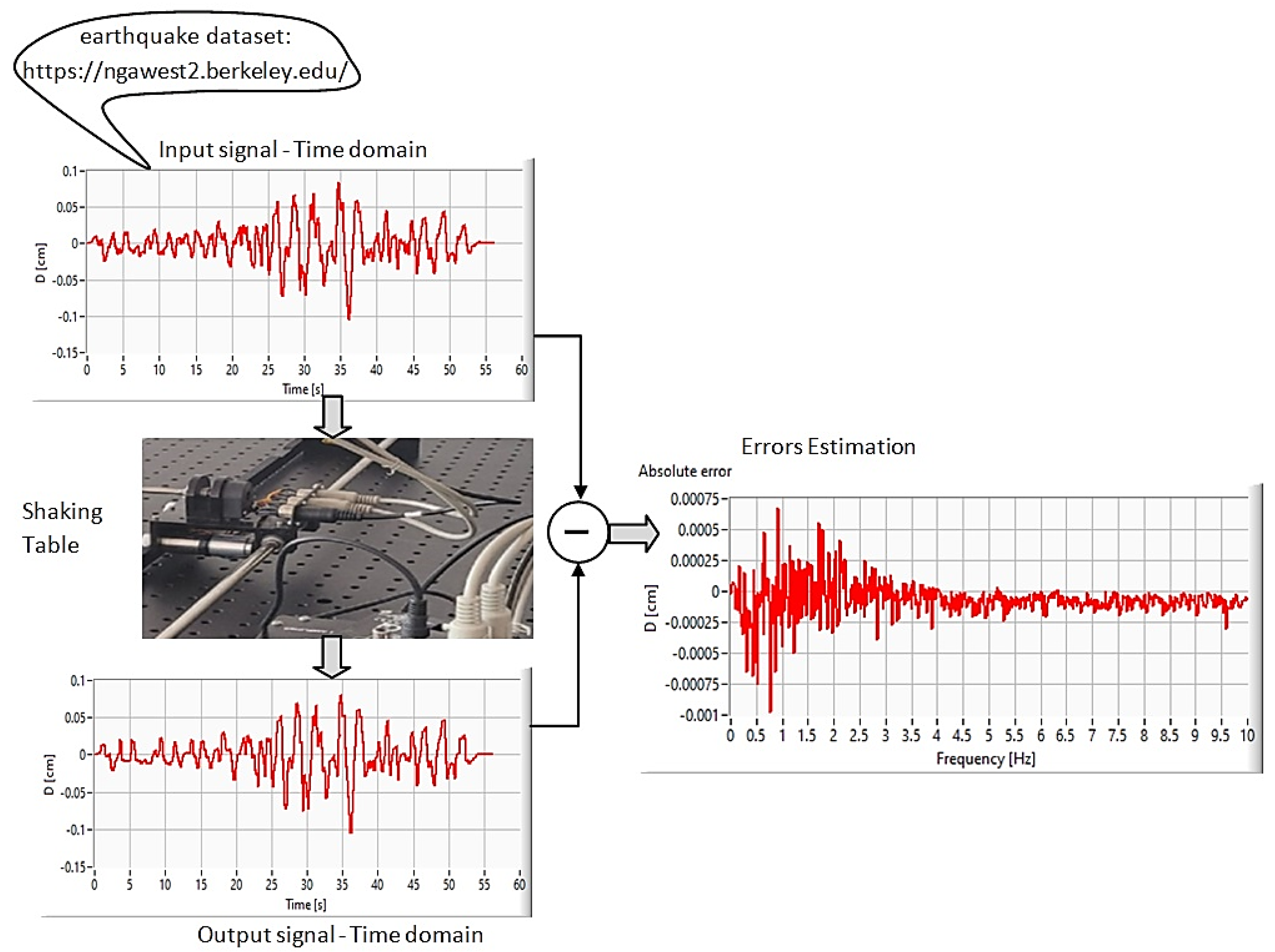
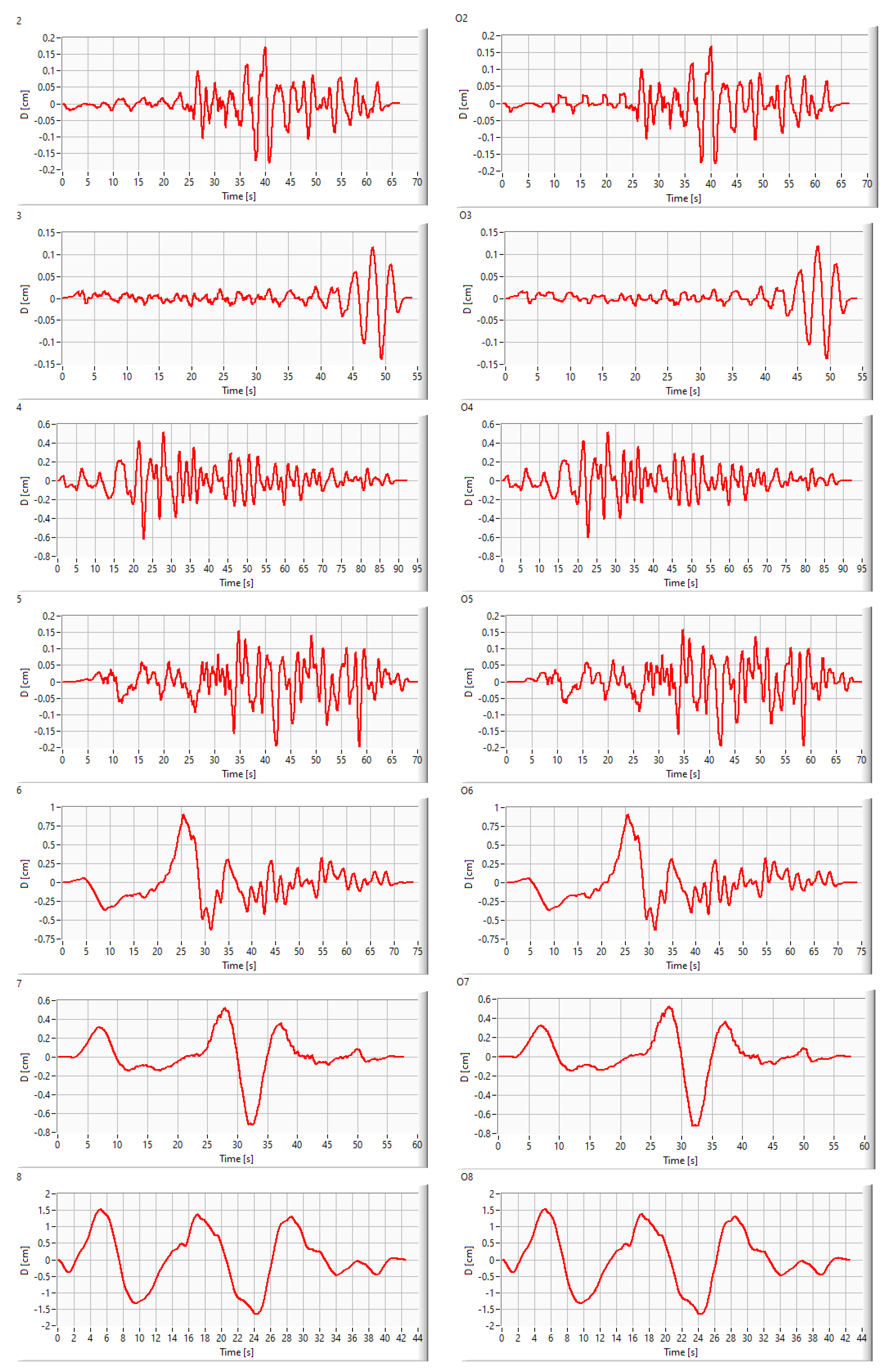
• Selecting the waveform that characterizes a real earthquake. The Pacific Earthquake Engineering Research Center (PEER) ground motion database was accessed, and based on certain selection criteria, such as event name, station name, rupture type, Rjb, and Rup, the earthquake was identified. For each event, the recordings provided the waveforms of acceleration, speed, and displacement in all three propagation directions x, y, and z. To evaluate the magnitude of the earthquake based on the P-wave, we only used the ground displacement wave in the vertical (z) direction.
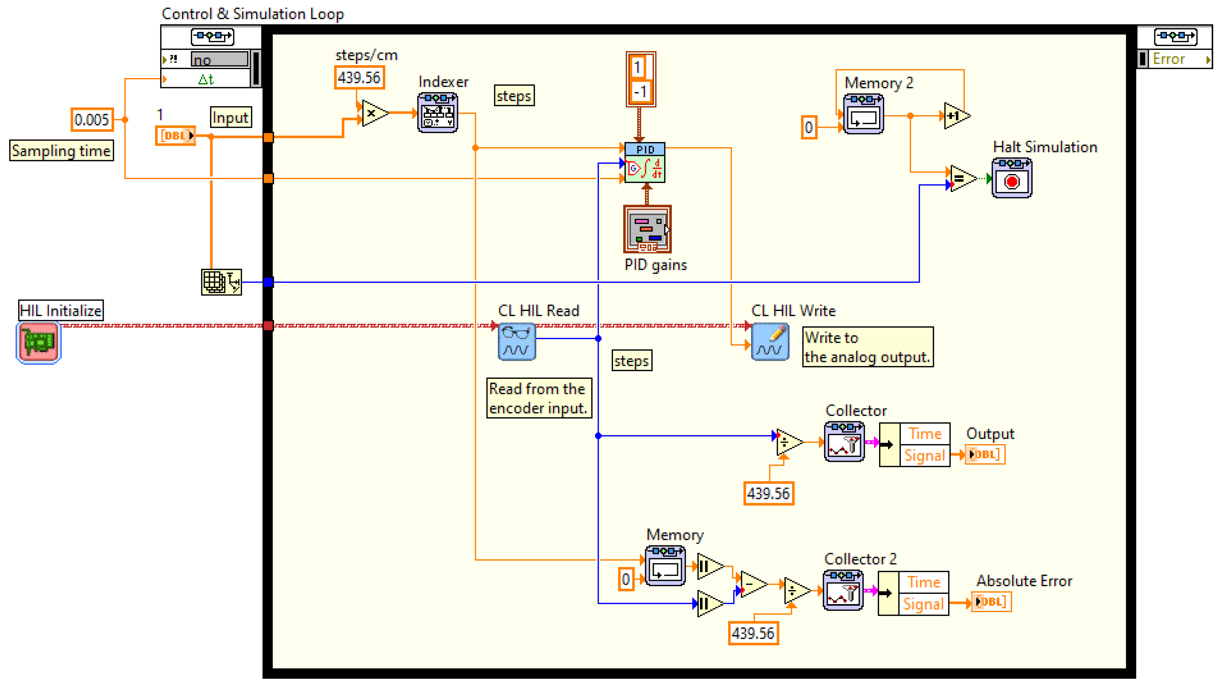
• Applying the command to the vibrating table. The points within the displacement waveform represent the instantaneous positions that the shaking table must reach. Positioning on each position was accomplished by completing a PID displacement control loop. The command was performed by transmitting a continuous voltage level to the DC motor, the voltage level being set by the PID controller based on the reaction. The reaction/feedback came from the displacement encoder.
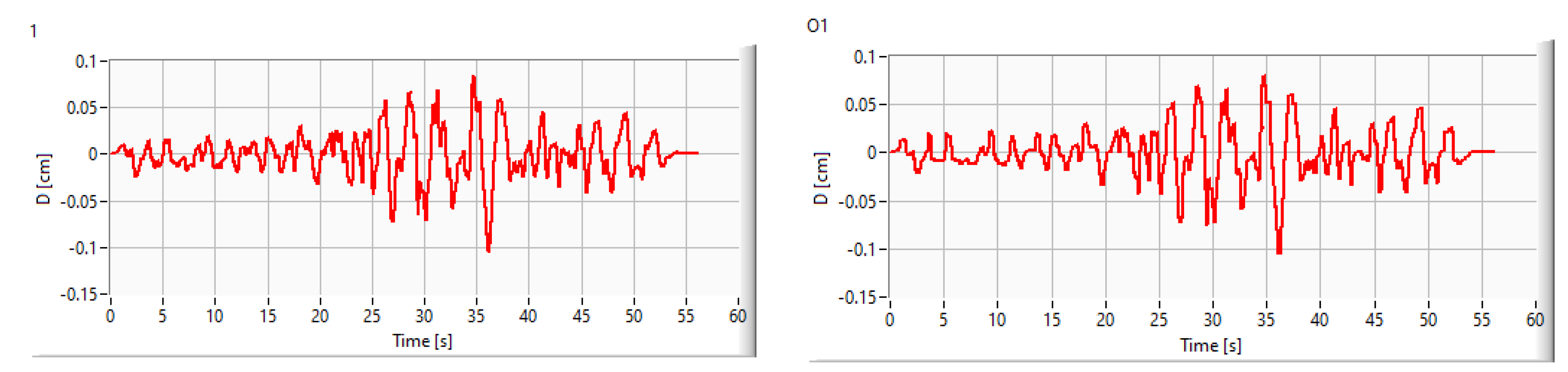
• Processing the output of the vibrating table was represented by the set of instantaneous points of displacement obtained from the encoder. Each value was obtained after completing the PID adjustment cycle.
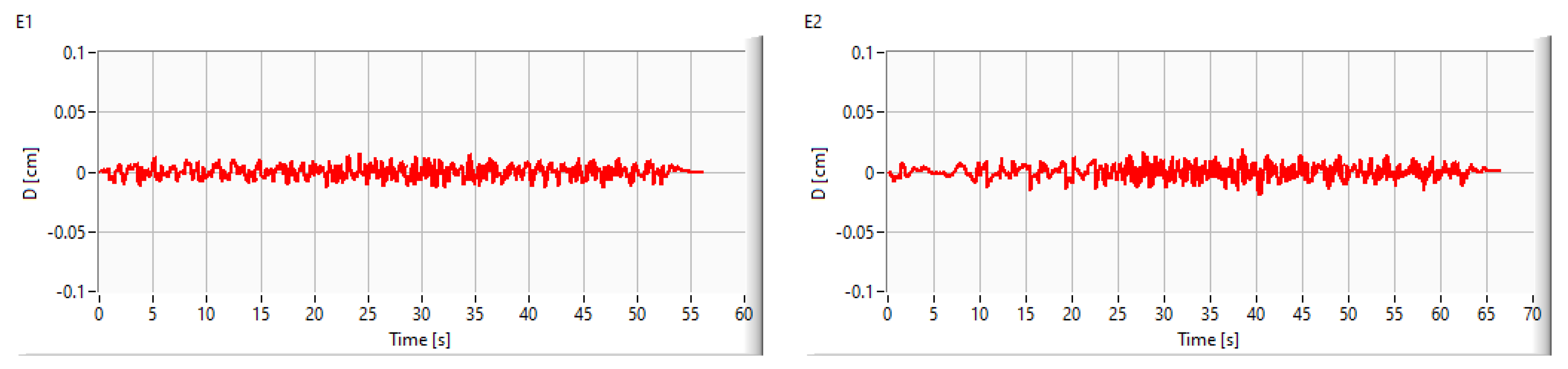
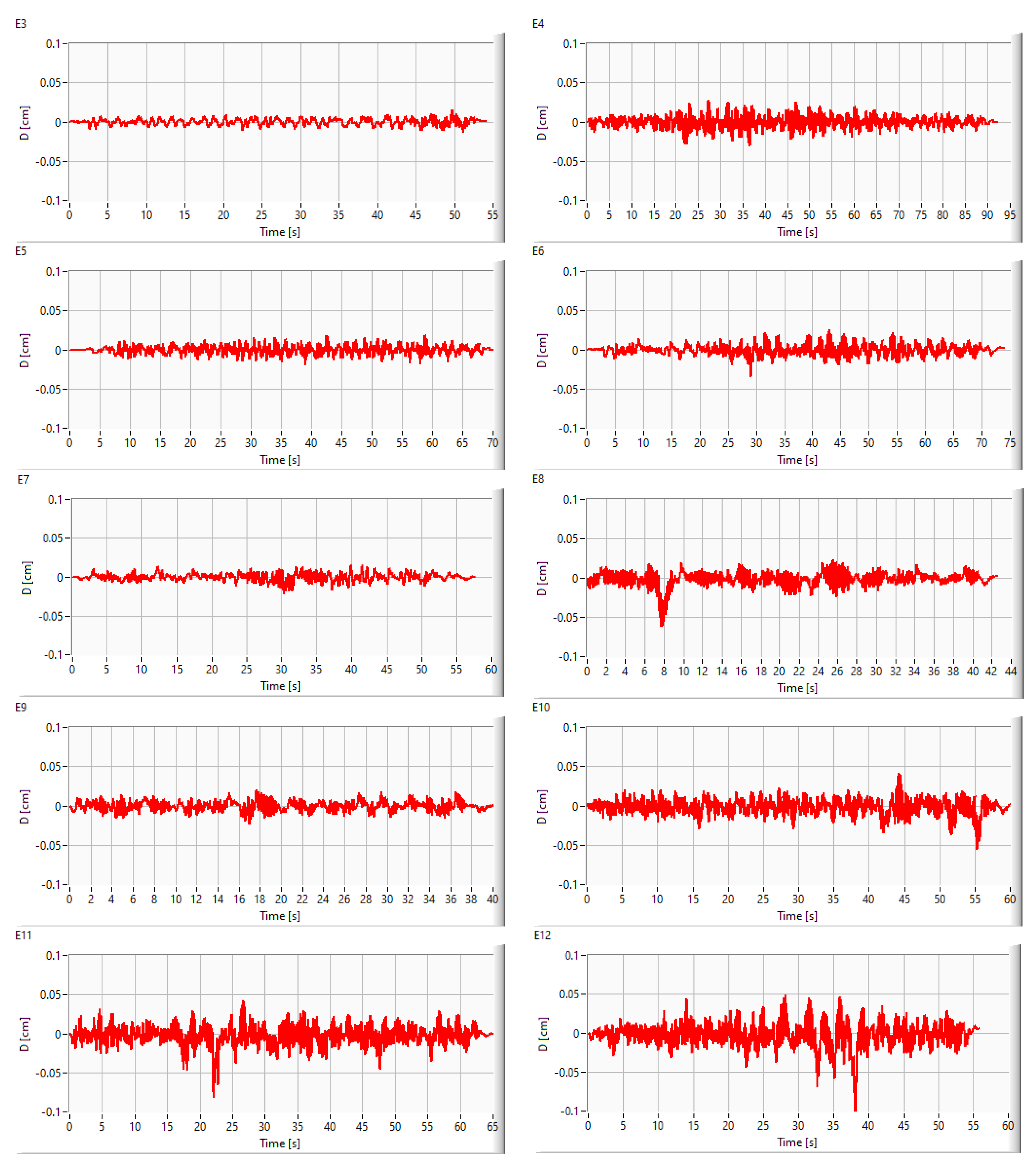
• Assessing the reproduction fidelity of the shaking table. The absolute error of reproduction of the vertical (z) ground displacement waveform was calculated as the difference between the instantaneous value of the waveform points applied to the input (reference) and the points obtained by using the shaking table.

3. Experimental Results

The objective of the experiment was to attest that the designed shake table could recreate the exact seismic activity with the data originally recorded, as shown in Table 1. Each of the 12 frequencies of the seismic events was simulated on input, and the results (outputs O) were computed (following the process in Figure 3). The duration of the event varied between 40 and 95 sec, depending on the seismic sequence recorded in the database. Shake table displacements were plotted for comparison in Figure 4: the graph from the left columns represents the waveforms of reference earthquakes (with parameters from Table 1), and the graph from the right column represents the displacement result registered through the encoder. Highlighting the first 3 s of the displacement tracking (the maximum time considered for P-wave detection [27]) reveals that the output peak amplitude of displacement was similar to the reference at each sequence of testing.

When analyzing the graphs displayed in Figure 5, we can see that the absolute errors of the proposed shaking table model, calculated between reference earthquakes and the measured samples, are very small. This means that the effect of each seismic motion is effectively transferred to the output.

To determine to what extent the earthquake’s energy is transferred to the system/sensor, the root mean square error (RMSE) was calculated and then normalized (NRMSE) (

Table 2. The displacement errors calculated for the 12 simulated earthquakes.

No	Name	Min (Input) (cm)	Max (Input) (cm)	Max–Min (Input) (cm)	Root Mean Square Error (RMSE) (cm)	Normalized Root Mean Square Error (NRMSE) (%)
1	Chi-Chi, Taiwan-02	−0.104	0.083	0.188	0.0046	2.48
2	Chi-Chi, Taiwan-02	−0.179	0.172	0.352	0.0049	1.41
3	Chi-Chi, Taiwan-02	−0.138	0.115	0.254	0.0037	1.45
4	Parkfield-02, CA	−0.613	0.514	1.128	0.0064	0.57
5	Parkfield-02, CA	−0.197	0.155	0.353	0.0049	1.39
6	Chi-Chi, Taiwan-03	−0.632	0.903	1.535	0.0060	0.39
7	Chi-Chi, Taiwan-03	−0.720	0.522	1.242	0.0045	0.36
8	San Fernando	−1.660	1.528	3.189	0.0087	0.27
9	San Fernando	−1.002	0.764	1.766	0.0055	0.31
10	El Alamo	−0.743	1.096	1.839	0.0093	0.51
11	Hector Mine	−2.592	1.931	4.524	0.0117	0.26
12	Lander	−2.099	2.606	4.705	0.0147	0.31

). The formula used to assess the absolute fit of the model to the reference seismic signal is:

$$RMSE=\sqrt{\frac{1}{n}{\sum }_{i=0}^{n-1}{(I}_i-O_i{)}^2}$$

(1)

where n is the number of samples, I is the input seismic displacement, and O is the output recorded displacement on the shaking table.

RMSE is a good measure of accuracy to compare forecasting errors of different models or model configurations for a particular variable, as it is scale-dependent [28]. The normalization of error between simulation (input) and observation (output) can be acheived by dividing RMSE into an interquartile range (usually 25% and 75%), by the standard deviation, by the mean, or by the difference between the max and min [29]. As the representation from Figure 3 shows some extreme values in the seismic input, the last variant was chosen from the NRMSE calculation. The results show that all scenarios provided low values (close to 0) for these errors, confirming a good-fitting model for the simulated pattern.

4. Discussion

Even EEWS can not predict a seism, but it can detect ground motion once the earthquake begins and send alerts to vulnerable areas before the destructive wave occurs. A real-time performance evaluation of EEWS involves, besides the average report time for the first alert, also the epicentral location and magnitude estimation [30]. EEWSs estimate earthquake magnitudes based on the initial few seconds after the P-wave arrival, but the final earthquake magnitude may differ, being determined by the initial rupture rather than the overall earthquake rupture process [31]. Special attention is paid to the development of precision methods for estimating the magnitude within an EEWS, because its conformity depends on the triggering of prevention actions, e.g., people to take shelter, automated systems to shut down or open. Related to this threshold of sensitivity and compliance, it can be appreciated that the designed shaking test table has good veracity, as recorded from the calculated errors in Table 2. The NRMSE decreasing with the increase of magnitude shows a good dynamic response of the system in the transverse direction.

Conducting the simulation on earthquakes of similar magnitude, less than or equal to 6 MW, but recorded at different stations in different geological conditions, discloses that NRMSE is strictly dependent on magnitude, but also on the seismic waveform. Thus, for the same earthquake of 5.9 MW magnitude (i.e., Chi Chi Taiwan 02), it was described by the parameters recorded at CHY065, CHY067, and CHY071 seismic stations located in the southwest of Taiwan at 22 km, with a respective 30 km distance between them, as different NRSMEs of 2.48%, 1.41%, and 1.45% respectively. For the Parkfield-02 event of magnitude 6 MW, it was described by parameters recorded at Hollister-Airport Bldg #3 and Salinas-County Hospital Gnds seismic stations with noticeable different NRMSEs of 0.57% and 1.39%, respectively. This difference is explained by the fact that the seismic waveform is strongly influenced by the length and the nonlinearity of the propagating medium, as geological elements (soil, rocks, sediments) are inhomogeneous and behave like mechanical deformable bodies. In other words, there is no coherence (similarity) of seismic waveforms recorded by stations in a far-field array when they are propagating through different heterogenic surfaces, at low frequencies. On the other side, seismic events with magnitudes higher than 6 MW, respective with larger rupture seizes, do not present significant differences for NRMSE: Chi-Chi Taiwan-03 earthquake, recorded simultaneously by the stations ILA006 and ILA007 located in the northeast of Taiwan, 7 km away from each other, provides close values of NRMSEs—0.39% and 0.36%, respectively; San Fernando earthquake (with the highest rupture size from the sequence) recorded simultaneously by the stations Isabella Dam (Aux Abut) and Bakersfield Harvey Aud, also provided close values of NRMSEs—0.27% and 0.31%, respectively. This apparent similarity is explained by the fact that for a given earthquake, the coherence of waveforms recorded by different stations improves with decreasing interstation distance and is to decay faster for earthquakes larger than 7 MW [32]. This behavior is known as the finite source effect when the magnification of a seismic rupture effect can be reduced from two-dimensional to one-dimensional integrals.

Compared to a similar experimental shaking table in [33], which was tested on three reference earthquakes through four hierarchical control methods (acceleration-based backstepping hierarchical control ABHC, acceleration-based backstepping hierarchical control with gain observer ABHCO, displacement-based backstepping hierarchical control DBHC, and displacement-based backstepping hierarchical control with gain observer DBHCO), the proposed shaking table with PID control provided similar results in terms of NRMSE on displacement.

Table 3. Displacement NRMSE comparison with a similar shaking table model.

	Xiao et al. Model					Proposed Model
Seismic Input	RSN 6-El Centro Array #9, 6.95 MW					El Centro Array #9, 6.8 MW
Shaking table control method	ABHC	ABHCO	DBHC	DBHO	PID	PID
NRMSE (%)	1.06	0.73	1.12	1.03	0.86	0.51
Seismic Input	RSN 79-Palmdale Fire Station, 6.61 MW					Bakersfield-Harvey Aud, 6.61 MW
Shaking table control method	ABHC	ABHCO	DBHC	DBHO	PID	PID
NRMSE (%)	2.10	1.48	2.17	2.04	1.54	0.27
Seismic Input	RSN 755-Coyote Lake Dam (SW Abut), 6.93 MW					El Centro Array #9, 6.8 MW
Shaking table control method	ABHC	ABHCO	DBHC	DBHO	PID	PID
NRMSE (%)	1.01	0.7	1.07	0.98	0.84	0.51

displays the tracking performance comparison between the two shaking table models, following three events from Table 1, close to those three tested in [33].

Being designed to test the response of EEWS seismic sensors (nonstructural elements), the proposed shaking table is 2 to 10 times smaller than regular ones and is mainly intended for structural element testing (scaled buildings or their components and cladding in part). A similar size uniaxial shaking table used in applications for nonstructural element testing, e.g., in [34], used for assessing the seismic impact on a freestanding ceramic object, was 100 times higher and the sliding carriage weighed 100 times more, requiring additional weight to avoid object’s overturning and for tracking 3D kinetic motion. As the proposed shaking table has a single degree of freedom (because the seismic sensors use only the vertical component of the seismic wave for the warning trigger), it requires one primary state variable controller, with which system stability is obtained as good as those with three control variables [35], with no damping issues. Consequently, the shaking table system’s cost is lower than similar size uniaxial shaking tables; approximately half of that specified in [36], where a moderate cost prototype is presented.

5. Conclusions

The modeling of test systems is as complex as the modeling of the phenomenon itself. Several conditions must be taken into account to give consistency to the experiment and to make the transition from empirical predictions to sustained predictions. If the model replicates a natural, hazard-type phenomenon, and with the potentially severe impact on the environment in which it occurs, as many dependent and independent variables as possible must be used. In the case of seismic wave reproduction, the reference must contain features that lead to simulation output as accurately as possible. The most common method to critically evaluate the seismic response of a structure or a sensitive component to ground motions is the shaking table test method.

Typical shaking tables undergo bearing capacity, tracking, and synchronization control precision problems. The high-fidelity reproduction of both acceleration and displacement tracking is complicated to achieve on most existing shaking tables with traditional control. Addressing this issue, this work aimed to realize a prototype intended for testing seismic sensors without bearing problems, and to validate its tracking performance. The proposed single-axis vibrating table tested under a sequence of 12 real earthquake signals proves that the control based on displacement feedback is accurate enough to assess the dynamic response of an EEWS sensor.

The furtherance of the present study, in which the fidelity of the earthquake movement transmission through the shaking table was established, will be acheived through a comparative dynamic response spectra analysis. The frequency spectrum of the outputs matching the reference earthquakes’ signal and the associated errors will be examined for the designed shaking table model. Subsequently, an adaptive PID controller will be designed and implemented to attain effective control of the shaking table.

References

1. Ammon, C.J.; Velasco, A.A.; Lay, T.; Wallace, T.C. Foundations of Modern Global Seismology, 2nd ed.; Lawrence, L., Ed.; Academic Press, Elsevier: London, UK, 2020. [Google Scholar] [CrossRef]
2. Fayaz, J.; Galasso, C. A deep neural network framework for real-time on-site estimation of acceleration response spectra of seismic ground motions. Comput.-Aided Civ. Infrastruct. Eng. 2023, 38, 87–103. [Google Scholar] [CrossRef]
3. Sollberger, D.; Igel, H.; Schmelzbach, C.; Edme, P.; van Manen, D.-J.; Bernauer, F.; Yuan, S.; Wassermann, J.; Schreiber, U.; Robertsson, J.O.A. Seismological Processing of Six Degree-of-Freedom Ground-Motion Data. Sensors 2020, 20, 6904. [Google Scholar] [CrossRef] [PubMed]
4. Williamson, A.; Lux, A.; Allen, R. Improving Out of Network Earthquake Locations Using Prior Seismicity for Use in Earthquake Early Warning. Bull. Seismol. Soc. Am. 2023, 113, 664–675. [Google Scholar] [CrossRef]
5. Cremen, G.; Galasso, C. Earthquake early warning: Recent advances and perspectives. Earth-Sci. Rev. 2020, 205, 103184. [Google Scholar] [CrossRef]
6. Chiang, Y.-J.; Chin, T.-L.; Chen, D.-Y. Neural Network-Based Strong Motion Prediction for On-Site Earthquake Early Warning. Sensors 2022, 22, 704. [Google Scholar] [CrossRef]
7. Licciardi, A.; Bletery, Q.; Rouet-Leduc, B.; Ampuero, J.P.; Juhel, K. Instantaneous tracking of earthquake growth with elastogravity signals. Nature 2022, 606, 319–324. [Google Scholar] [CrossRef]
8. D’Alessandro, A.; Scudero, S.; Siino, M.; Alessandro, G.; Mineo, R. Long-term monitoring and characterization of soil radon emission in a seismically active area. Geochem. Geophys. Geosyst. 2020, 21, e2020GC009061. [Google Scholar] [CrossRef]
9. Acceptance Criteria for Seismic Certification by Shake-Table Testing of Nonstructural Components ac156. Available online: https://icc-es.org/acceptance-criteria/ac156/ (accessed on 30 December 2022).
10. Lu, X.; Zou, Y.; Lu, W.; Zhao, B. Shaking table model test on Shanghai World Financial Center Tower. Earthq. Eng. Struct. Dyn. 2007, 36, 439–457. [Google Scholar] [CrossRef]
11. Nakashima, M.; Nagae, T.; Enokida, R.; Kajiwara, K. Experiences, accomplishments, lessons, and challenges of E-defense—Tests using world’s largest shaking table. Jpn. Archit. Rev. 2018, 1, 4–17. [Google Scholar] [CrossRef]
12. Damcı, E.; Şekerci, Ç. Development of a low-cost single-axis shake table based on Arduino. Exp. Tech. 2019, 43, 179–198. [Google Scholar] [CrossRef]
13. Baran, T.; Tanrikulu, A.K.; Dundar, C.; Tanrikulu, A.H. Construction and performance test of a low-cost shake table. Exp. Tech. 2011, 35, 8–16. [Google Scholar] [CrossRef]
14. Danish, A.; Ahmad, N.; Salim, M.U. Manufacturing and performance of an economical 1-D shake table. Civ. Eng. J. 2019, 5, 2019–2028. [Google Scholar] [CrossRef]
15. Quanser Shake Table II Product Information Sheet. Available online: https://quanserinc.app.box.com/s/fwi5ht5qjy4w34orwe384hbhscsj7zm1 (accessed on 13 January 2023).
16. Shao, X.; Enyart, G. Development of a versatile hybrid testing system for seismic experimentation. Exp. Tech. 2014, 38, 44–60. [Google Scholar] [CrossRef]
17. Shen, G.; Li, X.; Zhu, Z.; Tang, Y.; Zhu, W.; Liu, S. Acceleration tracking control combining adaptive control and off-line compensators for six-degree-of-freedom electro-hydraulic shaking tables. ISA Trans. 2017, 70, 322–337. [Google Scholar] [CrossRef]
18. Enokida, R.; Ikago, K.; Guo, J.; Kajiwara, K. Nonlinear signal-based control for shake table experiments with sliding masses. Earthq. Eng. Struct. Dyn. 2023, 52, 1908–1931. [Google Scholar] [CrossRef]
19. Antaki, G.; Gilada, R. Design Basis Loads and Qualification. In Nuclear Power Plant Safety and Mechanical Integrity: Design and Operability of Mechanical Systems, Equipment and Supporting Structures; Antaki, G., Gilada, R., Eds.; Butterworth-Heinemann; Elsevier: Oxford, UK, 2015; p. 30. [Google Scholar] [CrossRef]
20. Delgado, P.S.; Arêde, A.; Pouca, N.V.; Costa, A. Numerical Modeling of RC Bridges for Seismic Risk Analysis. In Handbook of Research on Computational Simulation and Modeling in Engineering; Miranda, F., Abreu, C., Eds.; IGI Global: Hershey, PA, USA, 2016; pp. 457–481. [Google Scholar] [CrossRef]
21. Rathje, E.M.; Faraj, F.; Russell, S.; Bray, J.D. Empirical Relationships for Frequency Content Parameters of Earthquake Ground Motions. Earthq. Spectra 2004, 20, 119–144. [Google Scholar] [CrossRef]
22. Liu, H.; Li, Y.; Zhang, Y.; Chen, Y.; Song, Z.; Wang, Z.; Qian, J. Intelligent tuning method of PID parameters based on iterative learning control for atomic force microscopy. Micron 2018, 104, 26–36. [Google Scholar] [CrossRef]
23. Puncello, I.; Caprili, S. Seismic Assessment of Historical Masonry Buildings at Different Scale Levels: A Review. Appl. Sci. 2023, 13, 1941. [Google Scholar] [CrossRef]
24. Bektaş, N.; Kegyes-Brassai, O. Development in Fuzzy Logic-Based Rapid Visual Screening Method for Seismic Vulnerability Assessment of Buildings. Geosciences 2023, 13, 6. [Google Scholar] [CrossRef]
25. Nievas, C.I.; Bommer, J.J.; Crowley, H.; van Elk, J.; Ntinalexis, M.; Sangirardi, M. A database of damaging small-to-medium magnitude earthquakes. J. Seism. 2020, 24, 263–292. [Google Scholar] [CrossRef]
26. Pacific Earthquake Engineering Research Center Ground Motion Database. Available online: https://ngawest2.berkeley.edu/ (accessed on 17 October 2022).
27. Khan, I.; Kwon, Y.-W. P-Detector: Real-Time P-Wave Detection in a Seismic Waveform Recorded on a Low-Cost MEMS Accelerometer Using Deep Learning. IEEE Geosci. Remote Sens. Lett. 2022, 19, 1–5. [Google Scholar] [CrossRef]
28. Christie, D.; Neill, S.P. Measuring and Observing the Ocean Renewable Energy Resource. In Comprehensive Renewable Energy, 2nd ed.; Letcher, T.M., Ed.; Elsevier: Amsterdam, The Netherlands, 2022; pp. 149–175. ISBN 9780128197349. [Google Scholar] [CrossRef]
29. Otto, S.A.; Kadin, M.; Casini, M.; Torres, M.A.; Blenckner, T. A quantitative framework for selecting and validating food web indicators. Ecol. Indic. 2018, 84, 619–631. [Google Scholar] [CrossRef]
30. Peng, C.; Jiang, P.; Ma, Q.; Wu, P.; Su, J.; Zheng, Y.; Yang, J. Performance evaluation of an earthquake early warning system in the 2019–2020 M 6.0 Changning, Sichuan, China, Seismic Sequence. Front. Earth Sci. 2021, 9, 699941. [Google Scholar] [CrossRef]
31. Zhu, J.; Li, S.; Song, J.; Wang, Y. Magnitude estimation for earthquake early warning using a deep convolutional neural network. Front. Earth Sci. 2021, 9, 653226. [Google Scholar] [CrossRef]
32. Zhou, T.; Meng, L.; Zhang, A.; Ampuero, J.P. Seismic Waveform-Coherence Controlled by Earthquake Source Dimensions. J. Geophys. Res. Solid Earth 2022, 127, e2021JB023458. [Google Scholar] [CrossRef]
33. Xiao, Y.; Pan, X.; Yang, T.T. Nonlinear backstepping hierarchical control of shake table using high-gain observer. Earthq. Eng. Struct. Dyn. 2022, 51, 3347–3366. [Google Scholar] [CrossRef]
34. Huang, B.; Günay, S.; Lu, W. Seismic assessment of freestanding ceramic vase with shaking table testing and performance-based earthquake engineering. J. Earthq. Eng. 2022, 26, 7956–7978. [Google Scholar] [CrossRef]
35. Ozcelik, O.; Conte, J.P.; Luco, J.E. Comprehensive mechanics-based virtual model of NHERI@ UCSD shake table—Uniaxial configuration and bare table condition. Earthq. Eng. Struct. Dyn. 2021, 50, 3288–3310. [Google Scholar] [CrossRef]
36. Damerji, H.; Yadav, S.; Sieffert, Y. Design of a Shake Table with Moderate Cost. Exp. Tech. 2022, 46, 365–383. [Google Scholar] [CrossRef]
Figure 1. Shaking table system components.
Designs 07 00072 g001
Figure 2. Displacement-based PID controller virtual instrument.
Designs 07 00072 g002
Figure 3. Experimental process diagram.
Designs 07 00072 g003
Figure 4. Shaking table cart displacement variation in time for the 12 sample earthquakes, on input vs. output.
Designs 07 00072 g004aDesigns 07 00072 g004bDesigns 07 00072 g004c
Figure 5. Absolute errors of displacement tracking on each of the 12 seismic events.
Designs 07 00072 g005aDesigns 07 00072 g005b