Article

Design of a Takagi–Sugeno Fuzzy Exact Modeling of a Buck–Boost Converter

by
Joelton Deonei Gotz
1,†,
Mario Henrique Bigai
2,†,
Gabriel Harteman
2,†,
Marcella Scoczynski Ribeiro Martins
2,†,
Attilio Converti
3,*,
Hugo Valadares Siqueira
2,†,
Milton Borsato
1,† and
Fernanda Cristina Corrêa
2,†
1
Graduate Program in Mechanical and Materials Engineering (PPGEM), Federal University of Technology—Paraná, Curitiba 81280-340, Brazil
2
Graduate Program in Electrical Engineering, Federal University of Technology—Paraná, Ponta Grossa 84017-220, Brazil
3
Department of Civil, Chemical and Environmental Engineering, University of Genoa, Pole of Chemical Engineering, Via Opera Pia, 15, 16145 Genoa, Italy
*
Author to whom correspondence should be addressed.
These authors contributed equally to this work.
Designs 2023, 7(3), 63; https://doi.org/10.3390/designs7030063
Submission received: 17 February 2023 / Revised: 3 May 2023 / Accepted: 7 May 2023 / Published: 9 May 2023
(This article belongs to the Special Issue Design and Optimization of Energy System Based on Demand Response)

Abstract

:
DC–DC converters are used in many power electronics applications, such as switching power supply design, photovoltaic, power management systems, and electric and hybrid vehicles. Traditionally, DC–DC converters are linearly modeled using a typical operating point for their control design. Some recent works use nonlinear models for DC–DC converters, due to the inherent nonlinearity of the switching process. In this sense, a standout modeling technique is the Takagi–Sugeno fuzzy exact method due to its ability to represent nonlinear systems over the entire operating range. It is more faithful to system behavior modeling, and allows a nonlinear closed-loop control design. The use of nonlinear models allows the testing of controllers obtained by linear methods to operate outside their linearization point, corroborating with robust controllers for specific applications. This work aims to perform the exact fuzzy Takagi–Sugeno modeling of a buck–boost converter with non-ideal components, and to design a discrete proportional–integral–derivative (PID) controller from the pole cancellation technique, obtained linearly, to test the controller at different operating points. The PID control ensured a satisfactory result compared with the stationary value of the different operating points, but it did not reach the desired transient response. Since the proposed model closely represents the operation of the buck–boost converter by considering the components’ non-idealities, other control techniques that consider the system’s nonlinearities can be applied and optimized later.

1. Introduction

Static power converters require control of their electrical variables, such as voltages, currents, and powers. To design suitable controllers, one needs to know the plant models of the power stage of the converter, which are usually in the form of transfer functions [1,2]. In this case, these transfer functions are obtained from linear differential equations, resulting from the linearization of nonlinear components bounded around the specific operating point of the converter power stage [2,3].
Several techniques have been proposed for obtaining the mathematical models of DC–DC static converters. One of the most popular is that using the average model in state space, presented by Midlebrook and Cuk in 1976 [4], using a linear approach.
Controller designs are developed based on the linear approach of DC–DC converters. One of the most popular topologies are PID controllers [5]. Recently, works have been using optimization techniques to tune PID controllers. Chander et al. [6] proposed an auto-tuned discrete PID controller for fast transient response applied to DC–DC converters. Mirzaei and Mojallali [7] used a chaotic particle swarm optimization (PSO) algorithm for a boost converter, an approach for auto-tuning an optimum startup response for a converter. Puchta et al. [8] proposed a robust Gaussian PID optimized via a genetic algorithm applied to a buck converter.
General fuzzy systems are used in control projects of complex dynamical systems. Recently, a novel adaptive fuzzy finite control method was proposed. Liu et al. [9] applied the fuzzy finite-time attitude control strategy to quadrotor UAVs under external disturbances and uncertain dynamics. The control technique achieved fast convergence speed, finite-time property, and was singularity-free, using the Lyapunov theorem to prove the closed-loop convergence.
Recently, works have used general fuzzy systems to design controllers in a linear approach for DC–DC converters. Gadari et al. [10] developed a variable gain fuzzy system to build robust controllers for DC–DC converters, managing variations in supply voltages and load.
In this way, there is also an interest in using models that consider non-linearities, i.e., applications in which control of the electrical parameters of DC–DC converters at different operating points is required. Based on this premise, the fuzzy Takagi–Sugeno (fuzzy TS) modeling approach is an exciting alternative for DC–DC converters [11].
Takagi and Sugeno proposed a fuzzy model representing a linear relationship between the input and output of a nonlinear model by locally valid, interpolated linear dynamical systems [12,13,14]. Fuzzy TS is widely used for nonlinear systems; one example is in Liu et al. [15]. The authors presented a suboptimal control with fuzzy TS methods and reinforcement learning (RL) for slow–fast coupled nonlinear systems. They segmented the systems into two problems, slow and fast, and used RL neural networks to reconstruct the non-measurable virtual subsystems through the original measurement systems for slow issues.
Ghany et al. [16] applied a combo of fuzzy TS and interval type-2 fuzzy sets (IT2-FSs) to build a new self-tuning fractional-order proportional–integral–derivative (PID). The IT2-FSs were used to tune the gains, while the fuzzy TS constructed the controller. Three types of tuning were established under disturbance changes, and the results proved that the proposed idea could control systems under disturbances and uncertainties. Torres-Pinzon et al. [17] performed a work applying fuzzy TS based on linear matrix inequalities (LMI) to regulate the voltage in switching systems. The authors carried out simulations and experiments with a prototype to validate the method.
In addition, some adaptive PID techniques can be used to improve the performance of traditional PID controllers. Borges et al. [18] and Itaborahy Filho et al. [19] used metaheuristic-based optimization to design some robust controllers.
The nonlinear model approximation performs better as the number of local models increases. However, the larger the number of local models, the more difficult it can become to control. Therefore, a representation close to the nonlinear model is desirable with as few local models as possible [1].
A generalized form of fuzzy TS modeling was proposed by Taniguchi et al., which is based on local models created from the regions that correspond to the maximum and minimum values of the system. Consequently, there is a decrease in the number of local models, defined by 2nl, where nl is the number of non-linearities in the system [20]. Recent investigations already use generalized fuzzy TS modeling applied to DC–DC converters, aiming to control the electrical parameters at different operating points [11,21,22,23,24]. In these works, exact fuzzy TS modelling was used to design fuzzy TS controllers analyzed by LMI and validated by the Lyapunov function.
This work aims to develop the fuzzy TS model of a buck–boost converter, considering the non-idealities of the components [2], to be a test framework of nonlinear scenarios for a discrete PID controller designed by the pole cancelling method obtained through the linear model [25,26]. The premise is that the controller output voltage obtained linearly and designed to control the voltage only at the typical operating point can be tested at different operating points. In addition, we desire to stabilize the output voltage as the reference voltage varies, taking the controller’s design parameters at the typical operating point as a metric.
The main contribution of this work is to obtain an exact nonlinear model, which considers the non-idealities of the components of a specific buck–boost converter, and to combine the traditional modeling and control techniques for DC–DC converters with the latest techniques.
This article is divided as follows: Materials and Methods are presented in Section 2; in Section 3 there is the Discrete PID Control Design; Section 4 shows the Results and Discussion; finally, in Section 5, the main conclusions and future perspectives are presented. A list of acronyms is shown in Table 1.

2. Materials and Methods

2.1. Buck–Boost Converter

2.1.1. Overview of DC–DC Converters

DC–DC converters can be conceptualized from a simple system consisting of a DC voltage source at the input, a DC–DC converter block, and a DC voltage source at the output. A DC–DC converter is an electronic circuit that processes a direct voltage at the input and transforms it into a direct voltage at the output, with active elements acting as switches, and passive components, usually inductors and capacitors, acting as controllers of the power flow between the sources [2].
The most commonly referenced non-isolated static DC–DC converter topologies in the literature are: buck, boost, buck–boost, Cúk, SEPIC, and zeta. The differentiation of the topologies is based on their static gain (M) and the polarity of the output voltage, as shown in Table 2, in which the static gain is given as a function of the duty-cycle (D).

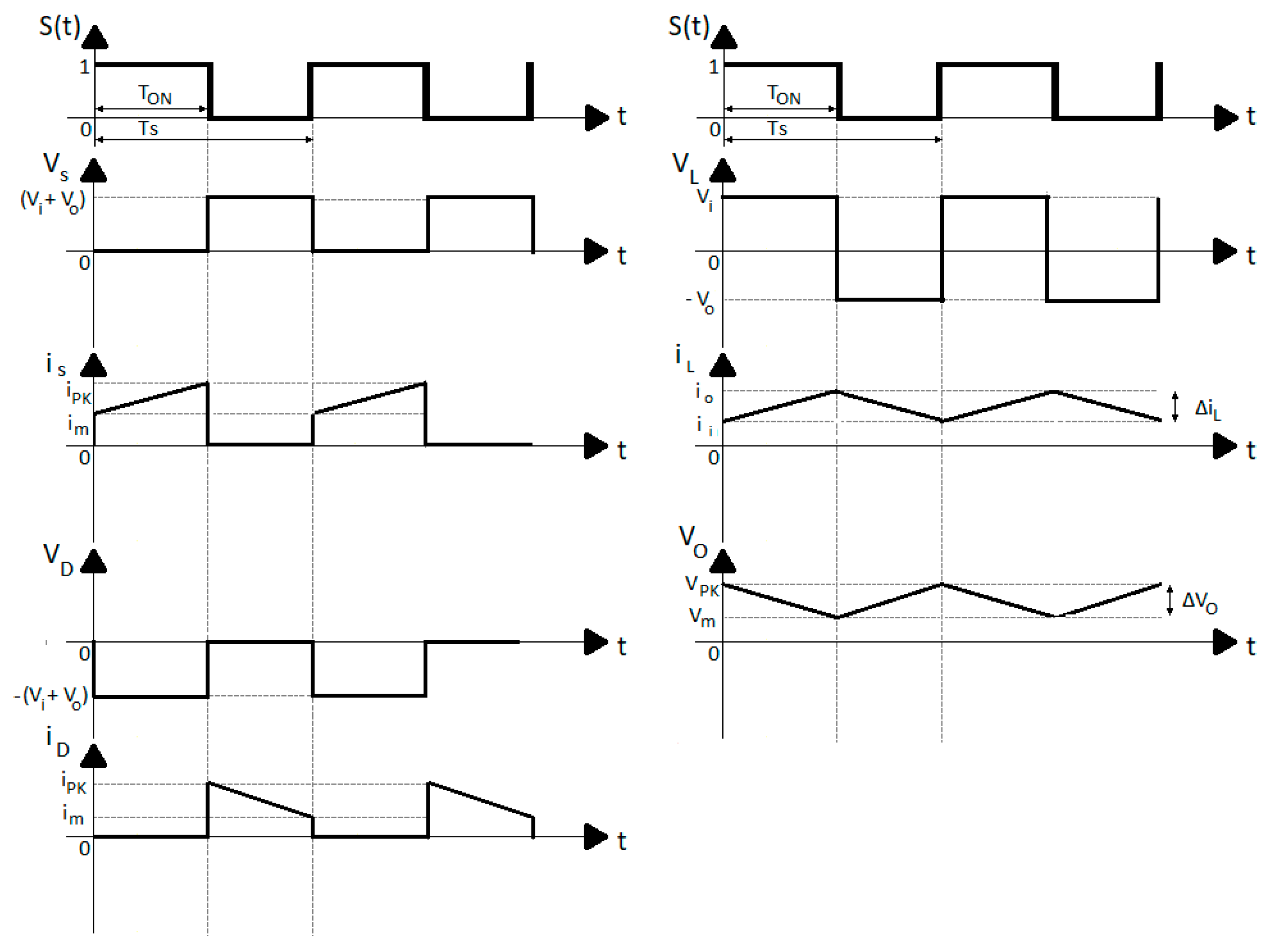
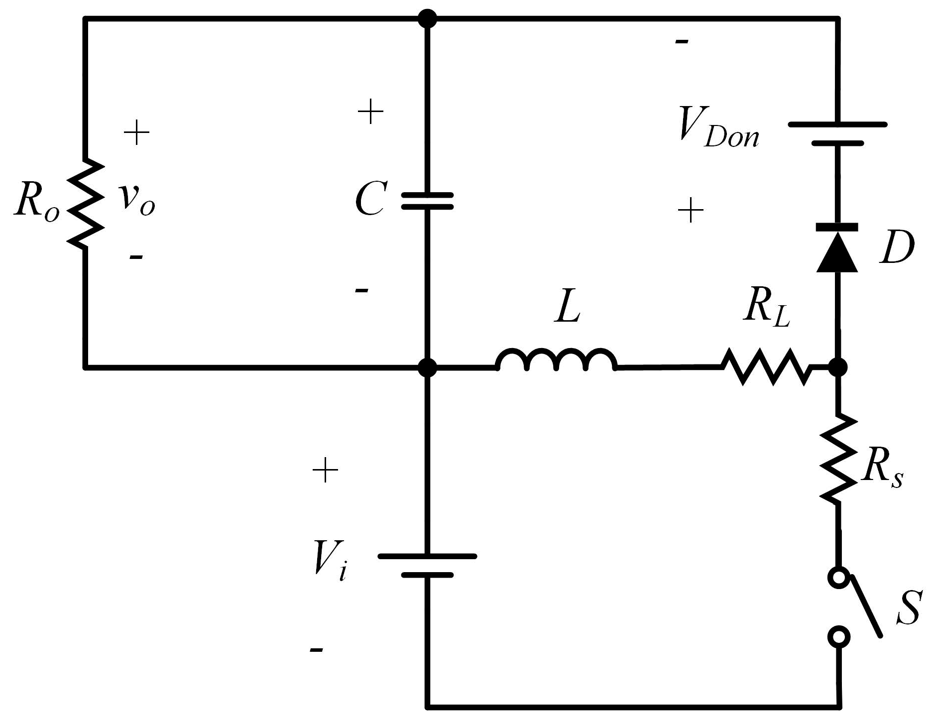
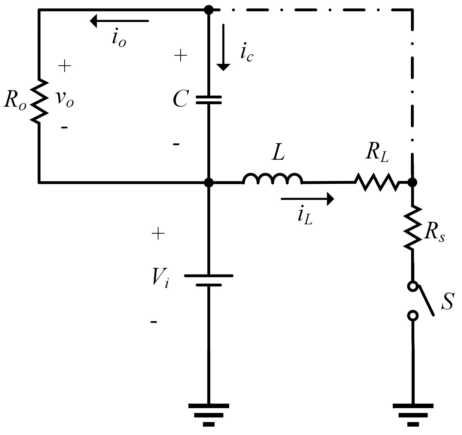
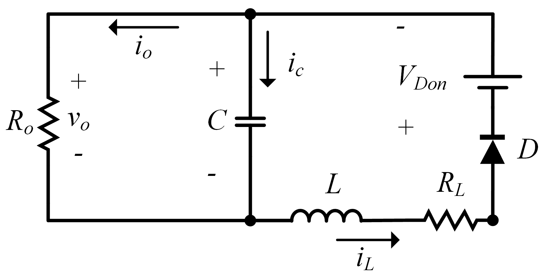
2.1.2. Buck–Boost Converter Project

The present work considers a buck–boost converter with the following design parameters: Vi = 24 V (input voltage), Vo = 14 V (output voltage), fs = 50 kHz (switching frequency), Ts = 20 ms (sampling time), Po = 100 W (output power), ∆Vo% = 1% (percent output voltage variation) and ∆IL% = 10% (percent current variation). For the continuous conduction mode (CCM), and initially considering the ideal converter represented in Figure 1, the corresponding waveforms of each electrical variable behave as depicted in Figure 2.
It is possible to consider the static gain of the buck–boost topology present in Table 2 as the ratio between the input and output voltage; isolating the duty-cycle, one can obtain the optimal value given by Equation (1):
D = V o ( V i + V o ) 0.3684
The variation in the inductor current is given by the difference between the average input current (Equation (2)) and output current (Equation (3)), according to the waveforms in Figure 2, assuming the ideal lossless converter (Pi = Po). Therefore, the nominal value of the inductor current (∆iL) and output voltage (∆Vo) variations are given by Equations (4) and (5), respectively.
i i = P o V i = 4.1667   A
i o = P o V o = 7.1429   A
Δ i L = Δ i L % · ( i i + i o ) = 1.131   A
Δ V o = Δ V o % · V o = 0.14   V
The load resistance (R) is calculated by Equation (6), with the ideal values of capacitance (C) and inductance (L) by Equations (7) and (8), respectively.
R = V o 2 P o = 1.96   Ω
C = i o · D Δ V o · f s = 375.9398   μ F
L = V i · D Δ i L · f s = 0.1564   mH
Consider non-idealities results in more accurate models, including an accurate stationary value analysis [2]. With the ideal components set, the schematic considering the non-idealities of the components is depicted in Figure 3.
In this case, Rs is the series resistance of the transistor (Mosfet), RL is the series resistance of the inductor, and VDON is the blocking voltage of the diode. The manufacturers define such parameters through the electrical characteristics of the specified components.
To define the actual capacitor, the commercial value that most closely matches the calculated theoretical capacitance was chosen, and supported by the maximum required voltage to which the theoretical capacitor will be subjected. The specified capacitor is the aluminum electrolytic capacitor B41858C5337M (C = 470 µF) [27].
The diode and transistor are specified from the maximum and minimum required voltages and currents, as shown in Figure 3. The Mosfet-SUP70090E is the transistor (Rs = 0.089 Ω) [28] and the MUR1620CT is the diode (VDON = 0.895 V) [29].

2.1.3. Mathematical Representation by State Space

The state space representation was carried out according to de Kremes et al. [2]; analyzing the circuit outlined in Figure 3, it has two operating stages: stage 1, with the Mosfet in conduction (Figure 4) and stage 2, with the diode in conduction (Figure 5).
The differential Equations (9) and (10) can be written for stage 1, while Equations (11) and (12) apply to stage 2:
L · d i L d t = ( R s + R L ) · i L + V i
C · d v o d t = v o R o
L · d i L d t = R s · i L V o V D
C · d v o d t = i L v o R o
It is possible to represent the equations in the form of a first-order linear differential equations system matrix, according to Equations (13) and (14), where d(t) is the system input:
[ ı L ˙ V o ˙ ] = [ ( R s + R L ) L 0 0 1 C · R o ] · [ i L V o ] + [ V i L 0 ] · d ( t )
[ ı L ˙ V o ˙ ] = [ R L L 1 L 1 C 1 C . R o ] · [ i L V o ] + [ V D O N L 0 ] · d ( t )
These differential equations can be presented in a compact form (Equations (15) and (16)), in which x is the output variables of the system (output voltage and current of the buck–boost converter), and u is the input variable (d(t)). The matrices A1, B1, A2 and B2 are represented by Equations (17)–(20), respectively:
X ˙ = A 1 · x + B 1 · u
X ˙ = A 2 · x + B 2 · u
A 1 = [ ( R s + R L ) L 0 0 1 C · R o ]
B 1 = [ V i L 0 ]
A 2 = [ R L L 1 L 1 C 1 C · R o ]
B 2 = [ V D O N L 0 ]
The matrices A1 and B1 refer to the operation interval (0, D × Ts) and the matrices A2 and B2 refer to the operation interval (D × Ts, Ts). Adding Equations (15) and (16), one can obtain Equation (21), which can also be written as Equation (22), considering Equations (23) and (24).
X ˙ = [ A 1 · D + A 2 · ( 1 D ) ] · x + [ B 1 · D + B 2 · ( 1 D ) ] · u
X ˙ = A · x + B · u
A = A 1 D + A 2 ( 1 D )
B = B 1 D + B 2 ( 1 D )
Replacing the circuit variables into Equation (21), we obtain the linearized state-space model of the buck–boost converter represented in Equations (25)–(29):
A = [ ( D · R s + R L ) L ( 1 D ) C ( 1 D ) L 1 C · R o ]
B = [ ( V i · D V D O N + V D O N · D ) L 0 ]
C = [ 0 1 1 0 ]
D = [ 0 0 ]
[ x 1 ( t ) ˙ x 2 ( t ) ˙ ] = [ ( R s · D + R L ) L ( 1 D ) L ( D 1 ) C 1 C · R o ] · [ x 1 ( t ) x 2 ( t ) ] + [ V i · D V D O N + V D O N · D L 0 ] · d ( t )

2.2. Takagi–Sugeno Fuzzy Modeling

Takagi and Sugeno proposed a fuzzy model representing a linear relationship between the input and output of a nonlinear model by locally valid, interpolated, linear dynamical systems [12].
The generalized form of fuzzy TS modeling was proposed by Taniguchi et al. [20], and is based on local models created from the operating regions that correspond to the maximum and minimum values of the system. The number of local models is related to the number of nonlinear functions of the system.
In the case of the state-space model adopted for the buck–boost converter, the nonlinear functions are the output voltage and current. To define its maximum and minimum values, Equations (30) and (31) are, respectively, the stationary values of the voltage and current, according to [2].
V o = R o · ( 1 D ) · [ D · V 1 ( 1 D ) · V D O N ] D · R s + R L + R o · ( 1 D ) 2
I o = ( 1 D ) · [ D · V 1 ( 1 D ) · V D O N ] D · R s + R L + R o · ( 1 D ) 2
To calculate the minimum values of the output current and voltage functions of the buck–boost converter, the variable D was replaced by 0 in Equations (30) and (31), leading to Equations (32) and (33):
V o M I N = R o · ( V D O N ) R L + R o = 0.8939   V
I o M I N = V D O N R L + R o = 0.4561   A
On the other hand, to calculate the respective maximum values, the variable D was replaced by 0.9, leading to Equations (34) and (35).
V o M A X = 0.1 · R o · [ 0.9 · V 1 ( 0.1 ) · V D O N ] 0.9 · R s + R L + R o · ( 0.1 ) 2 = 140.0219   V
I o M A X = 0.1 · [ 0.9 · V 1 ( 0.1 ) · V D O N ] 0.9 · R s + R L + R o · ( 0.1 ) 2 = 71.4397   A
To obtain the fuzzy TS model, it is necessary to use the Tanigushi technique, describing the equations so that the system input (d(t)) is isolated. By replacing D with d(t) in Equation (29) and isolating d(t), it is possible to obtain the model containing the non-linearities of the system represented by Equation (36):
[ x 1 ( t ) ˙ x 2 ( t ) ˙ ] = [ R L L 1 L 1 C 1 C · R o ] · [ x 1 ( t ) x 2 ( t ) ] + [ ( R s · x 1 + x 2 ) + V 1 V D O N L x 1 C ] · d ( t )
The equations that contain the non-linearities of the system are Equations (37) and (38):
ĝ 11 ( x ( t ) ) = ( R s · x 1 + x 2 ) + V 1 V D O N L
ĝ 21 ( x ( t ) ) = x 1 C
By substituting these equations into Equation (36), it is possible to rewrite it, considering the nonlinearities:
[ x 1 ( t ) ˙ x 2 ( t ) ˙ ] = [ 0 1 L 1 C 1 R C ] · [ x 1 ( t ) x 2 ( t ) ] + [ ĝ 11 ( x ( t ) ) ĝ 21 ( x ( t ) ) ] · d ( t )
Therefore, using the maximum and minimum values of the output current and voltage functions of the buck–boost converter, one can obtain the maximum and minimum values of the functions that contain the non-linearities, as in Equations (40)–(43):
b 111 = max { ĝ 11 ( x ( t ) ) } = 751.6158 × 10 3
b 112 = min { ĝ 11 ( x ( t ) ) } = 153.4716 × 10 3
b 211 = max { ĝ 21 ( x ( t ) ) } = 151.9994 × 10 3
b 212 = min { ĝ 21 ( x ( t ) ) } = 5715.2166
In this way, the nonlinear functions are represented from the pertinences associated with the maximum and minimum values, as shown in Equations (44) and (45):
ĝ 11 ( x ( t ) ) = α 1 ( x ( t ) ) · b 111 + α 2 ( x ( t ) ) · b 112 + α 3 ( x ( t ) ) · b 111 + α 4 ( x ( t ) ) · b 112
ĝ 21 ( x ( t ) ) = α 1 ( x ( t ) ) · b 211 + α 3 ( x ( t ) ) · b 212 + α 2 ( x ( t ) ) · b 211 + α 4 ( x ( t ) ) · b 212
It is necessary to consider the relevant local models, considering the scenarios of the global membership functions, to obtain the local linear models, represented by Equations (46)–(49).
  • Scenario 1 (B1):
α 1 ( x ( t ) ) = 1 , α 2 ( x ( t ) ) = 0 , α 3 ( x ( t ) ) = 0 , α 4 ( x ( t ) ) = 0
B 1 = [ b 111 b 211 ]
  • Scenario 2 (B2):
α 1 ( x ( t ) ) = 0 , α 2 ( x ( t ) ) = 1 , α 3 ( x ( t ) ) = 0 , α 4 ( x ( t ) ) = 0
B 2 = [ b 112 b 211 ]
  • Scenario 3 (B3):
α 1 ( x ( t ) ) = 0 , α 2 ( x ( t ) ) = 0 , α 3 ( x ( t ) ) = 1 , α 4 ( x ( t ) ) = 0
B 3 = [ b 111 b 212 ]
  • Scenario 4 (B4):
α 1 ( x ( t ) ) = 0 , α 2 ( x ( t ) ) = 0 , α 3 ( x ( t ) ) = 0 , α 4 ( x ( t ) ) = 1
B 4 = [ b 112 b 212 ]
The matrices A and C do not contain non-linearities, so for an accurate representation of the buck–boost converter with fuzzy TS models, they must have the same representation along the boundary of the model. Equations (50) and (51) present these ideas.
A 1 = A 2 = A 3 = A 4 = [ R L L 1 L 1 C 1 C · R o ]
C 1 = C 2 = C 3 = C 4 = [ 0 1 1 0 ]
Rewriting Equation (39) as a function of the local linear models and the pertinences, we have Equation (52):
x ˙ ( t ) = A ( α ) · x ( t ) + B ( α ) · u ( t ) ; y = C ( α ) · x ( t )
in which
A ( α ) = A 1 · α 1 + A 2 · α 2 + A 3 · α 3 + A 4 · α 4
B ( α ) = B 1 · α 1 + B 2 · α 2 + B 3 · α 3 + B 4 · α 4
C ( α ) = C 1 · α 1 + C 2 · α 2 + C 3 · α 3 + C 4 · α 4

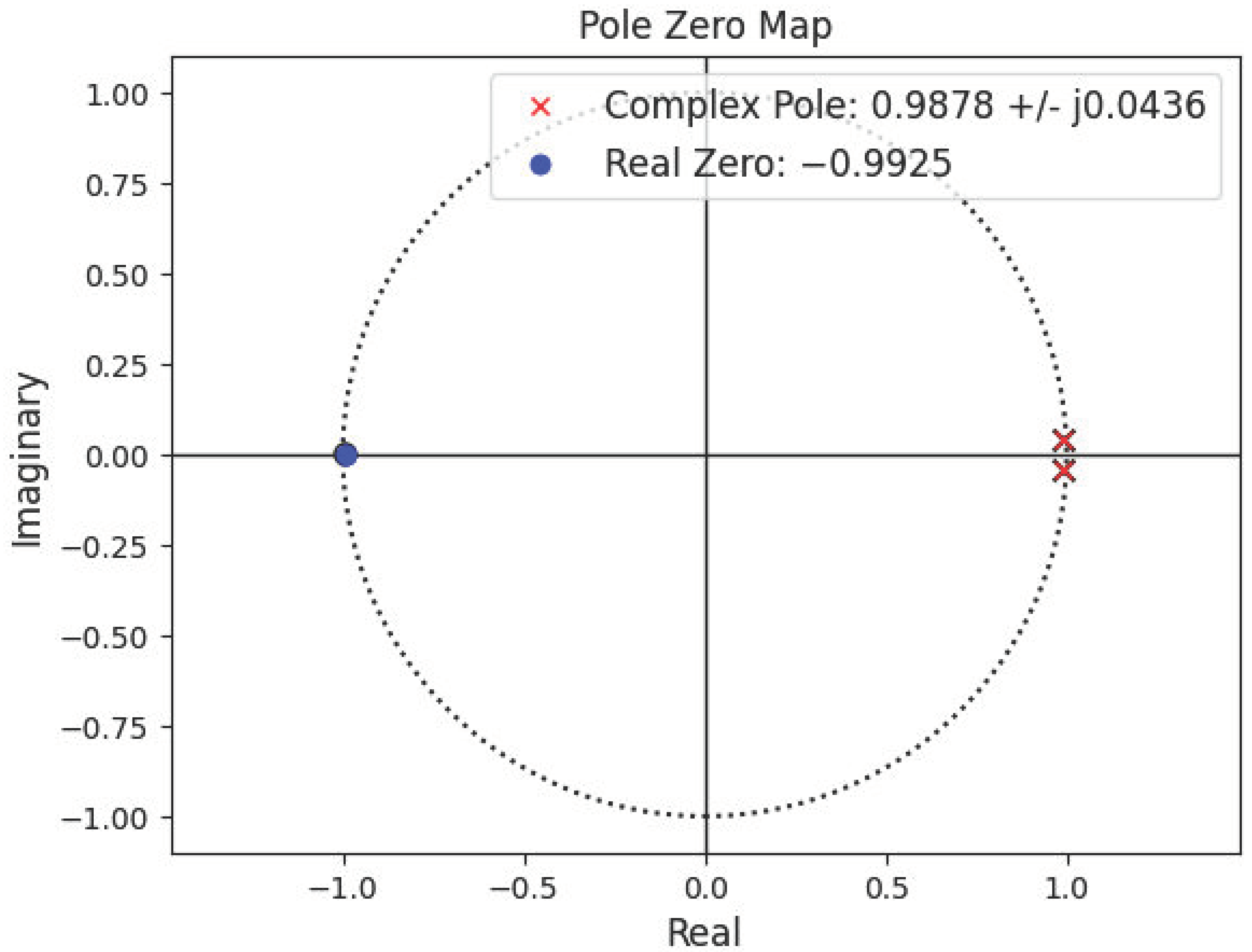
3. Discrete PID Control Design

As mentioned in Section 1, the output voltage of the discrete PID controller was designed for the linear model at the typical operating point, but the design aimed to control the output voltage at different operating points, by using the TS fuzzy exact model.
For the application of this control technique, the discrete transfer function of the output voltage is required [18,19]. This is obtained through the state-space linear model.
The linear modeling is found by replacing the duty cycle (D) with its numerical value. However, the linear model is limited to the linearization point, i.e., the transient and stationary performance parameters are relative to the linearization point.
Considering the non-idealities of the components, the duty-cycle value of the typical operating point of the buck–boost converter design is given by isolating the variable D from Equation (30) and replacing the output voltage by 14 V and the non-idealities of the components by the defined values. The typical operating point of the duty-cycle value is D ≈ 0.38472 [2].
Similarly, substituting the duty-cycle and the non-ideal component parameters into Equation (29) leads to the state-space model of the linearized buck–boost converter at the typical operating point, as depicted in Equation (53):
[ x 1 ( t ) ˙ x 2 ( t ) ˙ ] = [ 37.8774 3934.0008 1309.1015 1085.5406 ] · [ x 1 ( t ) x 2 ( t ) ] + [ 55 , 515.7359 0 ] · d ( t )
The continuous transfer function of the output voltage (Equation (54)) was extracted from Equation (53):
G v ( s ) = 7.268 × 10 7 s 2 + 1123 · s + 5.191 × 10 6
Discretizing Equation (54) using the zero-order hold (ZOH) method by applying a sampling period equal to the switching period of the converter (Ts = T = 20 ms), we obtain the discrete transfer function given by Equation (55).
G v ( z ) = 0.01442 · z + 0.01432 z 2 + 1.976 · z + 0.9778
To control the output voltage of the buck–boost converter, a discrete PID controller designed by the pole–zero cancellation method was proposed, following recent works [5,24,30]. Figure 6 contains the discrete pole–zero map, with the poles and zeros of the plant (Gv(z)).
Knowing the coordinates of the plant poles, the zeros of the discrete controller must be allocated near the plant poles to cancel the dominant poles’ transient effects and meet the requested design requirements [5].
Consider a discrete PID controller from the exact ZOH discretization whose transfer function is characterized by two fixed real poles at z = 0 and z = 1, and two adjustable conjugate complex zeros [1,31]. Equation (56) represents the discrete transfer function of the PID controller:
K ( z ) = ( k p + k d + k i ) · z 2 ( k p + 2 · k d ) · z + k d z · ( z 1 )
The literature establishes the design requirements for the controller in a closed loop as [31]:
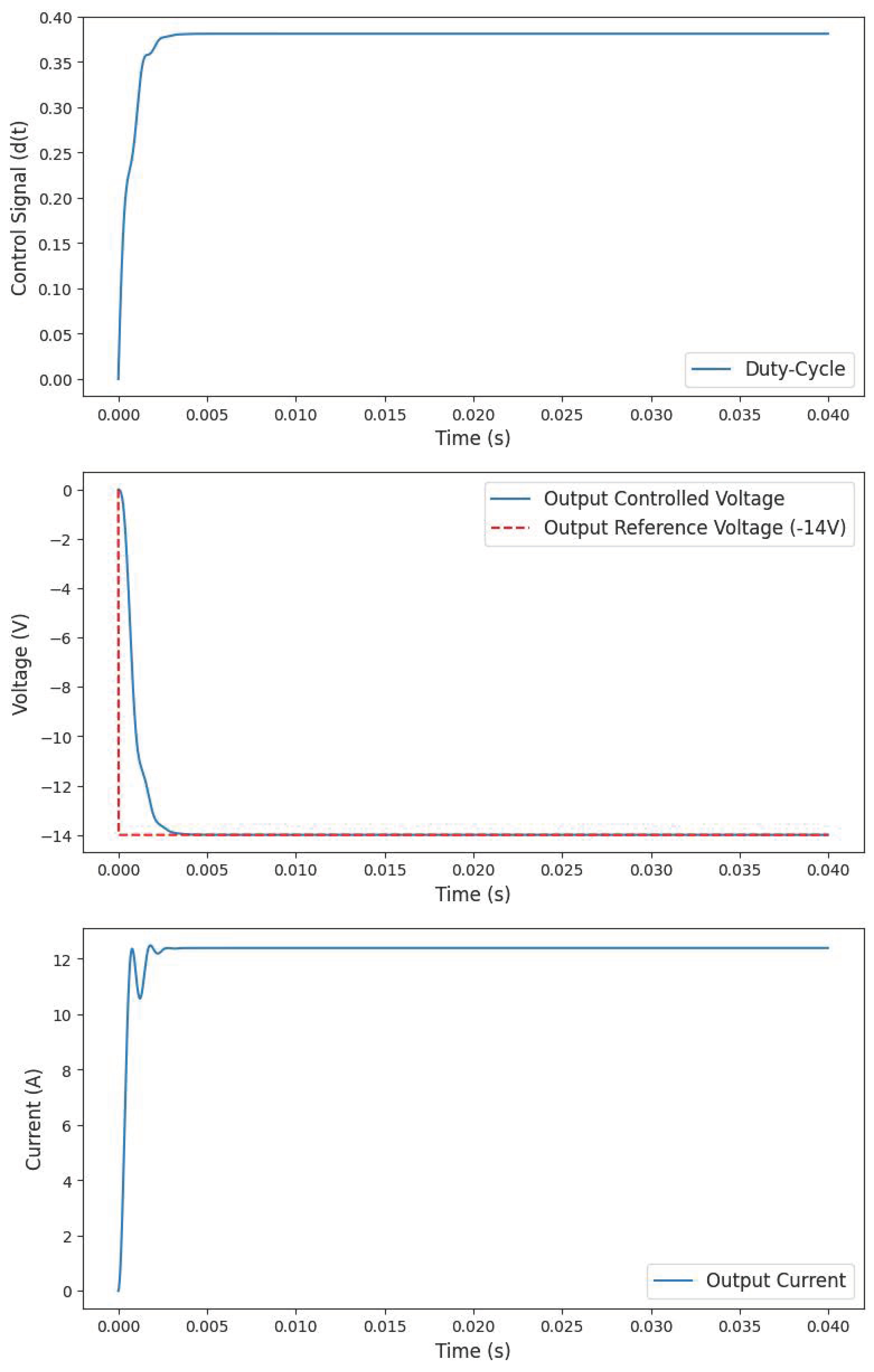
  • Zero stationary error for the reference voltages of −14 V (typical operating point).
  • Overshoot percentage of 10% (buck–boost design parameter).
From these considerations, the conjugate complex zeros of the PID controller (zeros PID = 0.96 ± j0.044) were allocated near the value of the plant poles, as shown in Figure 6. Moreover, we varied the direct gain of the controller, in order to satisfy the closed-loop design requirements, resulting in the following controller gains: kp = 0.02188, ki = 0.0011, and kd = 0.2771.
Figure 7 shows the closed-loop response of the buck–boost converter and the PID controller with the reference voltage at −14 V.

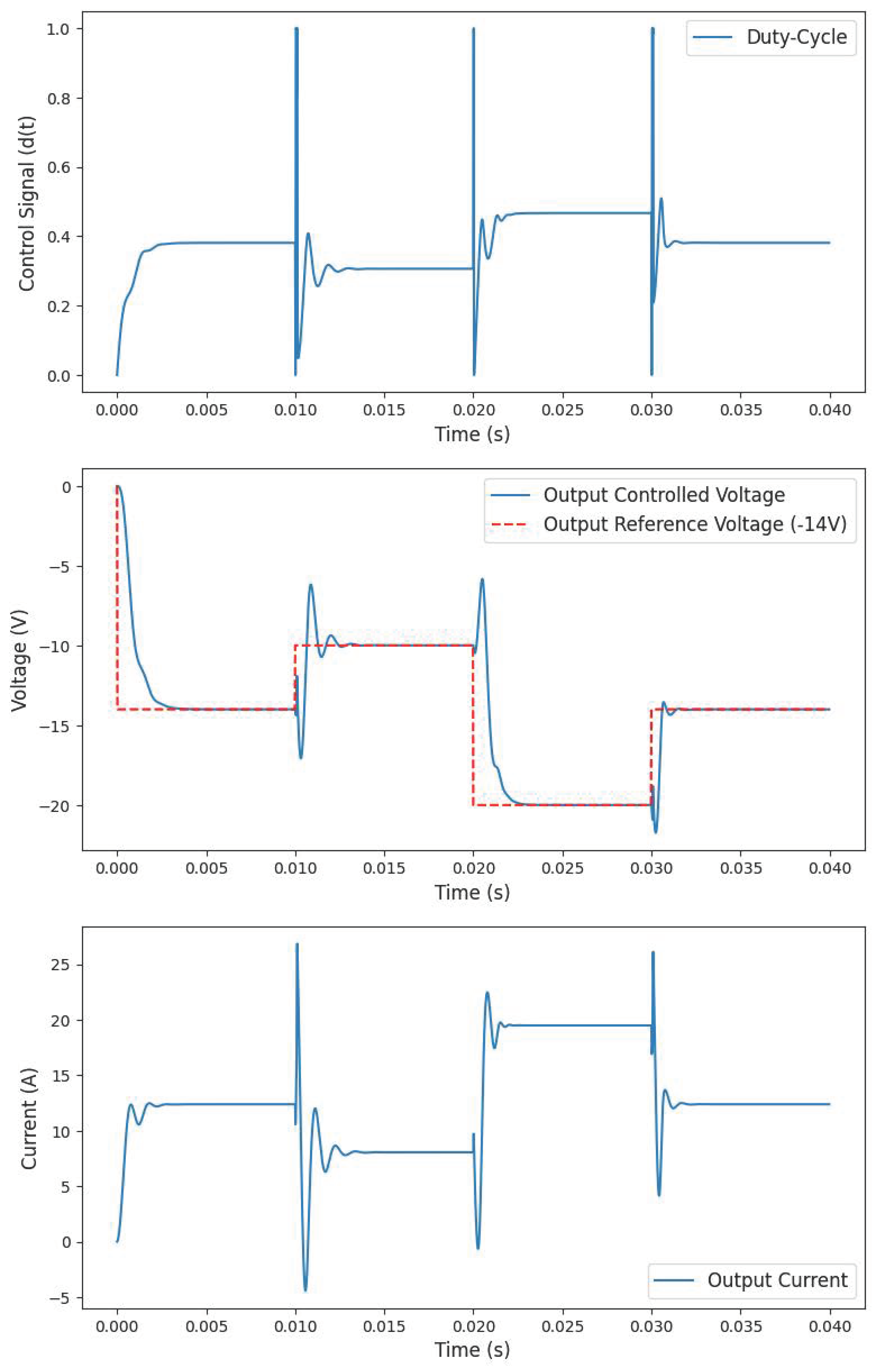
4. Results and Discussion

With the designed controller, stabilization tests were performed at values other than the typical output voltage point. Figure 8 illustrates the transient simulation of the buck–boost converter with the reference voltage changing initially from −14 V to −10 V at time t = 0.10 s to 20 V at time t = 0.20 s, and returning to 14 V at time t = 0.30 s. This simulation runs in a Python script using the Python control systems library [32].
Remarkably, the discrete PID controller was able to follow the reference voltage even when operating at a different point for which it was designed. However, comparing the response of the controller at its typical operating point with the previous works [5,6,7,24], the transient characteristics are compatible. However, if the performance at different operating points is compared with the works [11,21,22,23,24], the PID controller cannot obtain transient characteristics compatible with the specific operating point.
The fuzzy TS model of the buck–boost converter could represent the converter’s behavior at different operating points, enabling the testing of the discrete PID controller obtained by the method of pole cancellation operating under these conditions.
Such conditions highlight the fact that the linearized PID controller cannot manage the desired current-voltage tracking as designed at its typical operating point, Figure 7. As shown in Figure 8, overshoot requirements are extrapolated and compared to the typical operating point.
The linearized technique cannot handle a nonlinear approach, which changes the poles and zeros of the plant and directly impacts the controller performance. Furthermore, the control is limited to the output voltage, since it was obtained through the transfer function.
Thus, other control topologies can be proposed, such as optimized controllers, which are already applied to the control of DC–DC converters [6,7,8]. By aligning the optimized control techniques with the exact fuzzy TS model, the controllers can be optimized to find the best performance at different operating points.
Another control technique that can be applied from the fuzzy TS modeling is the control using the solution of linear matrix inequalities (LMI), which is a robust alternative control for nonlinear systems, because feedback is carried out by state space, enabling multiple control. This technique is currently applied in DC–DC converters in recent works [11,21,22,23,24,33]. The Lyapunov method validates and optimizes such a control technique, which can lead to a conservative solution [22].
We highlight the fact that the particle swarm optimization (PSO) or genetic algorithms (GA) are interesting candidates to minimize the absolute error integral (IAE) of the required operating conditions [8,34,35,36,37], and can be combined in adaptive PID controllers, such as GAPID, and fuzzy-PID to minimize the absolute error integral (AIE) in a non-linear approach.

5. Conclusions

DC–DC converters are widely used in a variety of engineering applications, such as switching power supplies, battery chargers, and power flow management for electric and hybrid vehicles. These converters are traditionally modeled and controlled using linear models. However, in applications where the converter is required to operate in different regions, traditional methods are not suitable, as they do not consider the inherent nonlinearity of the system.
This work obtained the exact fuzzy TS model of a buck–boost converter with specified non-idealities operating in continuous conduction mode. The obtained exact model was used to test the output voltage control found by traditional methods to check the linearly obtained controller in a non-linear model.
The discrete linear PID controller was able to follow the reference voltage signal, but did not achieve good transient performance parameters at the switching points. This occurs because, although the controller meets the requirement of zero stationary error at the various operating points, the controller parameters are not adjustable and do not consider the transient characteristics of the different operating points of the model. For future work, optimization techniques based on metaheuristics can be explored to design a robust controller applied to DC–DC converters with a non-linear approach provided by the fuzzy TS model.

Author Contributions

Conceptualization, M.H.B., J.D.G., G.H. and F.C.C.; methodology, M.H.B., J.D.G., G.H. and F.C.C.; software, M.H.B. and J.D.G.; validation, M.H.B. and F.C.C.; formal analysis, A.C. and H.V.S.; investigation, M.H.B., G.H. and M.S.R.M.; resources, A.C. and H.V.S.; data curation, M.B. and F.C.C.; writing—original draft preparation, M.H.B., G.H. and J.D.G.; writing—review and editing, M.S.R.M., A.C., M.B. and F.C.C.; visualization, M.H.B. and F.C.C.; supervision, A.C., H.V.S. and F.C.C.; project administration, F.C.C.; funding acquisition, A.C. All authors have read and agreed to the published version of the manuscript.

Funding

This study was financed in part by the Coordenação de Aperfeiçoamento de Pessoa de Nível Superior–Brasil (CAPES)-Finance Code 001. The authors thank the Brazilian National Council for Scientific and Technological Development (CNPq), process number 408053/2022-4, and Araucária Foundation, process number 51497, for their financial support.

Conflicts of Interest

The authors declare no conflict of interest.

References

  1. Ogata, K. Modern Control Engineering; Prentice Hall: Upper Saddle River, NJ, USA, 2010; Volume 5. [Google Scholar]
  2. de Kremes, W.J.; de Andrade, J.M.; Chokkalingam, B.; Illa Font, C.H.; Lazzarin, T.B. Input parallel–output parallel connected modular nonisolated DC-DC converters with current self-sharing capability operating in discontinuous conduction mode. Int. J. Circuit Theory Appl. 2023, 51, 340–359. [Google Scholar] [CrossRef]
  3. Syed, Z.A.; Wagner, J.R. Modeling and Control of a Multiple-Heat-Exchanger Thermal Management System for Conventional and Hybrid Electric Vehicles. Designs 2023, 7, 19. [Google Scholar] [CrossRef]
  4. Wester, G.W.; Middlebrook, R.D. Low-frequency characterization of switched DC-DC converters. IEEE Trans. Aerosp. Electron. Syst. 1973, AES-9, 376–385. [Google Scholar] [CrossRef]
  5. Cuoghi, S.; Ntogramatzidis, L.; Padula, F.; Grandi, G. Direct digital design of PIDF controllers with ComPlex zeros for DC-DC buck converters. Energies 2018, 12, 36. [Google Scholar] [CrossRef]
  6. Chander, S.; Agarwal, P.; Gupta, I. Auto-Tuned, Discrete PID Controller for DC-DC Converter for Fast Transient Response. In Proceedings of the India International Conference on Power Electronics 2010 (IICPE2010), New Delhi, India, 28–30 January 2011; pp. 1–7. [Google Scholar]
  7. Mirzaei, E.; Mojallali, H. Auto Tuning PID Controller Using Chaotic PSO Algorithm for a Boost Converter. In Proceedings of the 2013 13th Iranian Conference on Fuzzy Systems (IFSC), Qazvin, Iran, 27–29 August 2013; pp. 1–6. [Google Scholar] [CrossRef]
  8. Puchta, E.D.P.; Lucas, R.; Ferreira, F.R.V.; Siqueira, H.V.; Kaster, M.S. Gaussian Adaptive PID Control Optimized via Genetic Algorithm Applied to a Step-Down DC-DC Converter. In Proceedings of the 2016 12th IEEE International Conference on Industry Applications (INDUSCON), Curitiba, Brazil, 20–23 November 2016; pp. 1–6. [Google Scholar] [CrossRef]
  9. Liu, K.; Wang, R.; Dong, S.; Wang, X. Adaptive Fuzzy Finite-time Attitude Controller Design for Quadrotor UAV with External Disturbances and Uncertain Dynamics. In Proceedings of the 2022 8th International Conference on Control, Automation and Robotics (ICCAR), Xiamen, China, 8–10 April 2022. [Google Scholar]
  10. Gadari, S.K.; Kumar, P.; Mishra, K.; Bhowmik, A.R.; Chakraborty, A.K. Detailed analysis of fuzzy logic controller for second order DC-DC converters. In Proceedings of the 2019 8th International Conference on Power Systems (ICPS), Jaipur, India, 20–22 December 2019. [Google Scholar]
  11. Hazil, O.; Bououden, S.; Chadli, M.; Filali, S. Fuzzy Model Predictive Control of DC-DC Converters. In AETA 2013: Recent Advances in Electrical Engineering and Related Sciences; Springer: Berlin/Heidelberg, Germany, 2014; pp. 423–432. [Google Scholar] [CrossRef]
  12. Takagi, T.; Sugeno, M. Fuzzy identification of systems and its applications to modeling and control. IEEE Trans. Syst. Man Cybern. 1985, SMC-15, 116–132. [Google Scholar] [CrossRef]
  13. Reda, A.; Vásárhelyi, J. Design and Implementation of Reinforcement Learning for Automated Driving Compared to Classical MPC Control. Designs 2023, 7, 18. [Google Scholar] [CrossRef]
  14. Neto, P.S.D.M.; Firmino, P.R.A.; Siqueira, H.; Tadano, Y.D.S.; Alves, T.A.; De Oliveira, J.F.L.; Marinho, M.H.D.N.; Madeiro, F. Neural-based ensembles for particulate matter forecasting. IEEE Access 2021, 9, 14470–14490. [Google Scholar] [CrossRef]
  15. Liu, X.; Yang, C.; Luo, B.; Dai, W. Suboptimal control for nonlinear slow-fast coupled systems using reinforcement learning and Takagi–Sugeno fuzzy methods. Int. J. Adapt. Control Signal Process. 2021, 35, 1017–1038. [Google Scholar] [CrossRef]
  16. Ghany, M.A.A.; Bahgat, M.E.; Refaey, W.M.; Sharaf, S. Type-2 fuzzy self-tuning of modified fractional-order PID based on Takagi–Sugeno method. J. Electr. Syst. Inf. Technol. 2020, 7, 2. [Google Scholar] [CrossRef]
  17. Torres-Pinzón, C.; Paredes-Madrid, L.; Flores-Bahamonde, F.; Ramirez-Murillo, H. LMI-Fuzzy control design for non-minimum phase DC-DC converters: An application for output regulation. Appl. Sci. 2021, 11, 2286. [Google Scholar] [CrossRef]
  18. Borges, F.G.; Guerreiro, M.; Monteiro, P.E.S.; Janzen, F.C.; Corrêa, F.C.; Stevan, S.L., Jr.; Siqueira, H.V.; Kaster, M.d.S. Metaheuristics- Based Optimization of a Robust GAPID Adaptive Control Applied to a DC Motor-Driven Rotating Beam with Variable Load. Sensors 2022, 22, 6094. [Google Scholar] [CrossRef] [PubMed]
  19. Itaborahy Filho, M.A.; Puchta, E.; Martins, M.S.; Antonini Alves, T.; Tadano, Y.d.S.; Corrêa, F.C.; Stevan, S.L., Jr.; Siqueira, H.V.; Kaster, M.d.S. Bio-inspired optimization algorithms applied to the GAPID control of a Buck converter. Energies 2022, 15, 6788. [Google Scholar] [CrossRef]
  20. Taniguchi, T.; Tanaka, K.; Ohtake, H.; Wang, H.O. Model construction, rule reduction, and robust compensation for generalized form of Takagi-Sugeno fuzzy systems. IEEE Trans. Fuzzy Syst. 2001, 9, 525–538. [Google Scholar] [CrossRef] [PubMed]
  21. Cervantes, M.H.; Montiel, M.F.; Marín, J.A.; Anguiano, A.T.; Ramírez, M.G. Takagi-Sugeno Fuzzy Model for DC-DC Converters. In Proceedings of the 2015 IEEE International Autumn Meeting on Power, Electronics and Computing (ROPEC), Ixtapa, Mexico, 4–6 November 2015; pp. 1–6. [Google Scholar] [CrossRef]
  22. Nachidi; Meriem; El Hajjaji, A.; Bosche, J. An enhanced control approach for dc–dc converters. Int. J. Electr. Power Energy Syst. 2013, 45, 404–412. [Google Scholar] [CrossRef]
  23. Tatikayala, V.K.; Dixit, S. Takagi-Sugeno Fuzzy based Controllers for Grid Connected PV-Wind-Battery Hybrid System. In Proceedings of the 2021 International Conference on Recent Trends on Electronics, Information, Communication & Technology (RTEICT), Bangalore, India, 27–28 August 2021. [Google Scholar]
  24. Quispe, B.B.; e Melo, G.d.A.; Cardim, R.; Ribeiro, J.M.d.S. Single-Phase Bidirectional PEV Charger for V2G Operation with Coupled-Inductor Cuk Converter. In Proceedings of the 2021 22nd IEEE International Conference on Industrial Technology (ICIT), Valencia, Spain, 10–12 March 2021; Volume 1. [Google Scholar]
  25. Abe, S.; Zaitsu, T.; Obata, S.; Shoyama, M.; Ninomiya, T. Pole-Zero-Cancellation Technique for DC-DC Converter. In Advances in PID Control; IntechOpen: London, UK, 2011. [Google Scholar] [CrossRef]
  26. Awada, A.; Younes, R.; Ilinca, A. Optimized active control of a smart cantilever beam using genetic algorithm. Designs 2022, 6, 36. [Google Scholar] [CrossRef]
  27. TKDs. Aluminum Electrolytic Capacitors, 2019. Rev. 1. Available online: https://www.tdk-electronics.tdk.com/inf/20/30/db/aec/B41895.pdf (accessed on 10 January 2023).
  28. Siliconix, V. N-Channel 100 V (D-S) MOSFET, 2016. Rev. A. Available online: https://www.vishay.com/docs/62634/si7252dp.pdf (accessed on 10 January 2023).
  29. ON Semiconductor. Ultrafast Rectifiers 16 Amperes, 100600 Volts, 2015. Rev. 8. Available online: https://www.onsemi.com/pdf/datasheet/mur1620ct-d.pdf (accessed on 10 January 2023).
  30. Puchta, E.D.P.; Bassetto, P.; Biuk, L.H.; Itaborahy Filho, M.A.; Converti, A.; Kaster, M.d.S.; Siqueira, H.V. Swarm-Inspired Algorithms to Optimize a Nonlinear Gaussian Adaptive PID Controller. Energies 2021, 14, 3385. [Google Scholar] [CrossRef]
  31. Ogata, K. Discrete-Time Control Systems; Prentice-Hall, Inc.: Hoboken, NJ, USA, 1995. [Google Scholar]
  32. Fuller, S.; Greiner, B.; Moore, J.; Murray, R.; van Paassen, R.; Yorke, R. The Python Control Systems Library (Python-Control). In Proceedings of the 2021 60th IEEE Conference on Decision and Control (CDC), Austin, TX, USA, 14–17 December 2021. [Google Scholar]
  33. Siqueira, H.; Macedo, M.; Tadano, Y.d.S.; Alves, T.A.; Stevan, S.L., Jr.; Oliveira, D.S., Jr.; Marinho, M.H.N.; Neto, P.S.G.d.M.; Oliveira, F.L.d.; Luna, I.; et al. Selection of Temporal Lags for Predicting Riverflow Series from Hydroelectric Plants Using Variable Selection Methods. Energies 2020, 13, 4236. [Google Scholar] [CrossRef]
  34. Lian, K.Y.; Liou, J.J.; Huang, C.Y. LMI-based integral fuzzy control of DC-DC converters. IEEE Trans. Fuzzy Syst. 2006, 14, 71–80. [Google Scholar] [CrossRef]
  35. Siqueira, H.; Santana, C.; Macedo, M.; Figueiredo, E.; Gokhale, A.; Bastos-Filho, C. Simplified binary cat swarm optimization. Integr. Comput. Aided Eng. 2021, 28, 35–50. [Google Scholar] [CrossRef]
  36. Santos, P.; Macedo, M.; Figueiredo, E.; Santana, C.J.; Soares, F.; Siqueira, H.; Maciel, A.; Gokhale, A.; Bastos-Filho, C.J. Application of PSO-Based Clustering Algorithms on Educational Databases. In Proceedings of the 2017 IEEE Latin American Conference on Computational Intelligence (LA-CCI), Arequipa, Peru, 8–10 November 2017; pp. 1–6. [Google Scholar] [CrossRef]
  37. Puchta, E.D.P.; Siqueira, H.V.; Kaster, M.D.S. Optimization Tools Based on Metaheuristics for Performance Enhancement in a Gaussian Adaptive PID Controller. IEEE Trans. Cybern. 2020, 50, 1185–1194. [Google Scholar] [CrossRef] [PubMed]
Figure 1. Ideal buck–boost converter. Adapted from [2].
Designs 07 00063 g001
Figure 2. Waveforms of a buck–boost converter operating in continuous conduction mode. Adapted from [2].
Designs 07 00063 g002
Figure 3. Buck–boost converter with non-idealities. Adapted from [2].
Designs 07 00063 g003
Figure 4. Stage 1: Mosfet in conduction (0, D × Ts). Adapted from [2].
Designs 07 00063 g004
Figure 5. Stage 2: Diode in conduction (D × Ts, Ts). Adapted from [2].
Designs 07 00063 g005
Figure 6. Pole–zero map of output voltage discrete transfer function.
Designs 07 00063 g006
Figure 7. Closed-loop response with typical point operation (Vre f = −14 V).
Designs 07 00063 g007
Figure 8. Closed-loop response by varying the reference voltage.
Designs 07 00063 g008
Table 1. Acronyms.
Table 1. Acronyms.
TermAcronym
DC–DCDirect Current
TSTakagi–Sugeno
PIDProportional–integral–derivative
RLReinforcement learning
LMILinear matrix inequality
PSOParticle swarm optimization
Table 2. Static gain of main topologies of non-isolated DC–DC static converters. Adapted from [2].
TopologyStatic Gain (M)
BuckD
Boost1/(D − 1)
Buck–BoostD/(1 − D)
CúkD/(1 − D)
SEPICD/(1 − D)
ZetaD/(1 − D)
Disclaimer/Publisher’s Note: The statements, opinions and data contained in all publications are solely those of the individual author(s) and contributor(s) and not of MDPI and/or the editor(s). MDPI and/or the editor(s) disclaim responsibility for any injury to people or property resulting from any ideas, methods, instructions or products referred to in the content.

