CanDiag: Fog Empowered Transfer Deep Learning Based Approach for Cancer Diagnosis

Abstract

Breast cancer poses the greatest long-term health risk to women worldwide, in both industrialized and developing nations. Early detection of breast cancer allows for treatment to begin before the disease has a chance to spread to other parts of the body. The Internet of Things (IoT) allows for automated analysis and classification of medical pictures, allowing for quicker and more effective data processing. Nevertheless, Fog computing principles should be used instead of Cloud computing concepts alone to provide rapid responses while still meeting the requirements for low latency, energy consumption, security, and privacy. In this paper, we present CanDiag, an approach to cancer diagnosis based on Transfer Deep Learning (TDL) that makes use of Fog computing. This paper details an automated, real-time approach to diagnosing breast cancer using deep learning (DL) and mammography pictures from the Mammographic Image Analysis Society (MIAS) library. To obtain better prediction results, transfer learning (TL) techniques such as GoogleNet, ResNet50, ResNet101, InceptionV3, AlexNet, VGG16, and VGG19 were combined with the well-known DL approach of the convolutional neural network (CNN). The feature reduction technique principal component analysis (PCA) and the classifier support vector machine (SVM) were also applied with these TDLs. Detailed simulations were run to assess seven performance and seven network metrics to prove the viability of the proposed approach. This study on an enormous dataset of mammography images categorized as normal and abnormal, respectively, achieved an accuracy, MCR, precision, sensitivity, specificity, f1-score, and MCC of 99.01%, 0.99%, 98.89%, 99.86%, 95.85%, 99.37%, and 97.02%, outperforming some previous studies based on mammography images. It can be shown from the trials that the inclusion of the Fog computing concepts empowers the system by reducing the load on centralized servers, increasing productivity, and maintaining the security and integrity of patient data.

1. Introduction

A frequent and dangerous kind of cancer in women, breast cancer, affects around 36% of females. It is the most prevalent kind of cancer in women and the second-leading cause of cancer-related mortality, after lung cancer. According to the World Health Organization (WHO), breast cancer claims the lives of more than 2 million women each year. Breast cancer is the only illness that results in as many disability-adjusted life years (DALYs) of impairment for women worldwide. After puberty, breast cancer can affect women of any age, while the chance of getting it is increased later in life. According to the research, there will be more than 3 million new cases of breast cancer each year, and by 2040 there will be a 40% increase, with more than 1 million fatalities, i.e., a 50% increase in comparison with the year 2020 [1,2].

The core challenge of chronic illness research is image classification with deep learning, whereby several objective categories are created and a trained model to recognize each type is produced [3]. An early breast cancer diagnosis is the best way to prevent death and eventually lower healthcare costs. Technologies for the early detection and diagnosis of breast cancer are constantly developing to provide patients with less intrusive procedures and precise diagnoses. 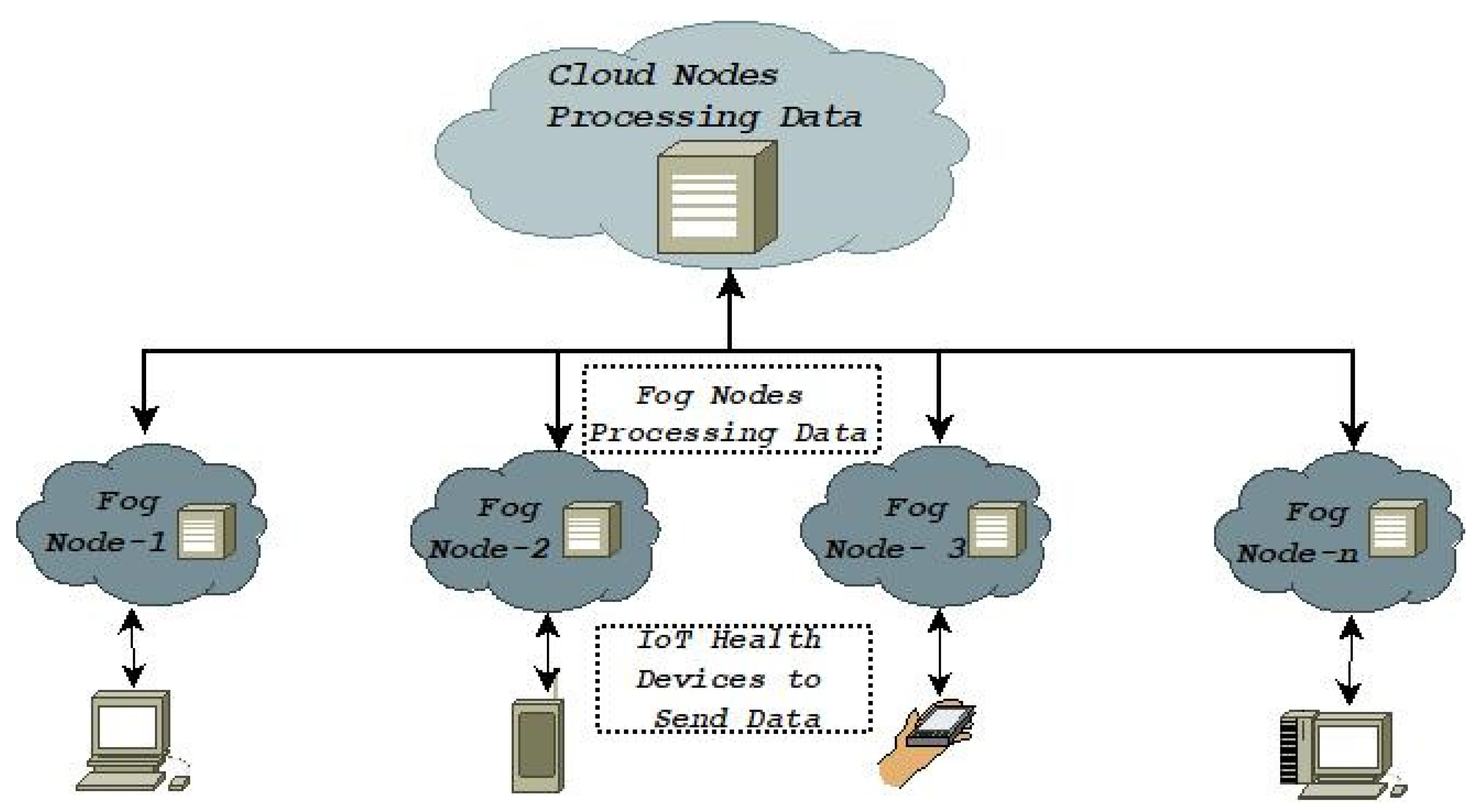Mammography is the key factor in reducing breast cancer mortality [4,5]. The Internet of Things (IoT) provides a wide variety of applications in the healthcare industry due to the quick advancement of smart medical equipment. However, these systems are built on a centralized connection with Cloud servers, increasing security and privacy risks. Fog computing, a distributed computing architecture developed by CISCO that integrates Cloud computing into the network to get around incompatible formats, keeps data computation, processing, and applications between the Cloud and the network’s edges [6]. Fog computing has brought up age-old problems such as host node movement, data center exchange, data security, and robustness. Additionally, in today’s healthcare system, people who are aged, ill, or physically challenged are becoming more in need of a trustworthy continuous health monitoring system. According to several research studies, the remote health monitoring system is what enables healthcare professionals to efficiently and quickly monitor patients’ health [7,8]. Figure 1 shows the Fog–Cloud-based distributions to IoT Healthcare systems.

Despite the abundance of literature studies on the subject of breast cancer diagnosis and classification, relatively few works have been performed on the classification of breast cancer using mammography images and on a distant instantaneous diagnosis based on Fog computing ideas. Despite the importance of image data pre-processing and segmentation approaches for breast cancer detection, ensemble deep learning (EDL) models perform in a wide variety of other contexts. In this study, we used publicly available mammography pictures from the Mammographic Image Analysis Society (MIAS) repository to train a novel transfer deep learning (TDL) enabled automated assistance system for breast cancer diagnosis and classification enabled with a Fog computing strategy. The data were pre-processed before being provided to the model. Transfer learning (TL) techniques, such as GoogleNet, ResNet50, ResNet101, In-ceptionV3, AlexNet, VGG16, and VGG19, were integrated with convolutional neural networks (CNNs), a common deep learning (DL) methodology. These TDLs were combined with the feature reduction method principal component analysis (PCA) and the classifier support vector machine (SVM) to further enhance their prediction capabilities. We ran comprehensive simulations to test how well the proposed model works in practice.

The important contributions of this study are listed below:

• The effectiveness of the proposed system is shown and evaluated in several scenarios, including predictive analysis, network capacity, low latency, bandwidth, secrecy, integrity, and protection;
• Automated remote diagnosis of benign and malignant breast cancer;
• Designed a TDL-based algorithm to analyze mammograms for the early detection of breast cancer;
• Installation of an IoT-based healthcare monitoring system utilizing Fog computing for real-time analysis;

The remainder of this manuscript is structured as shown below. Information about the pertinent work is provided in Section 2. The methods and datasets employed in this proposed study are described in detail in Section 3. Section 4 discusses the implementation of the experimental setting and the elaborate architectural design of the proposed work. Section 5 of the manuscript includes a discussion of the experiments and comparative analysis. Finally, in Section 6, we draw some final findings and provide some recommendations about the proposed approach.

2. Existing Works

Khan et al. [9] examined the effectiveness of six methods for extracting directional features for mass classification issues in digital mammograms. The feature extraction methods were assessed using the MIAS database’s extracted ROIs. The resultant imbalanced datasets were effectively classified using SELwSVM, or Successive Enhancement Learning-based weighted support vector machine.

Hepsag et al. [10] used DL with CNN to categorize anomalies in mammography pictures as benign or malignant by utilizing two distinct databases, namely, mini-MIAS and BCDR, and they found that accuracy, precision, recall, and f-score values were between roughly 60% and 72%. The authors used pre-processing techniques that included cropping, augmentation, and balancing picture data to enhance their findings.

To help doctors make an early diagnosis, Ting et al. [11] introduced CNN Improvement for Breast Cancer Classification (CNNI-BCC). Through studies, it has been found that CNNI-BCC is capable of accurately classifying incoming medical photos of patients as benign, malignant, or normal.

Mohanty et al. [12] developed a hybrid CAD framework to classify suspicious areas as normal, aberrant, benign, or malignant. The proposed framework consisted of four computational elements: A number of classifiers, such as SVM, KNN, NB, and C4.5, were used to categorize inputs as normal, abnormal, benign, or malignant on MIAS and DDSM; ROI generation using cropping operation; texture feature extraction using contourlet transformation; forest optimization algorithm (FOA), a wrapper-based feature selection algorithm, to select the best features.

Abd-Elmegid [13] presented a Fog computing-based architecture for predicting breast cancer prognosis. The proposed architecture employed the BCOAP model as a prediction tool and solved the issue of handling massive volumes of data in real-time without taxing the Cloud’s data center by employing Fog nodes to carry these out.

Chougrad et al. [14] proposed a tailored label choice system that calculates the best level of confidence for each visual notion. The authors used the CBIS-DDSM, BCDR, INBreast, and MIAS benchmark datasets to show the efficacy of their methodology and compared the findings to those of other widely used baselines.

The Fuzzy c-means clustering approach was utilized by Xu et al. [15] in their enhanced semi-supervised tumor identification system, which provides a pathological degree tree based on 10 3D and 2D tumor variables. The design of Fog computing also distributed a significant amount of complex data processing using the medical CT images of 143 individuals, including 452 tumors.

Zhu et al. [16] used DL approaches to build a technique for enhancing low-dose mammography picture quality. The CNN model for it focused on lowering the noise in low-dose mammography. After some practice, it may provide a picture of good quality from a low-dose mammogram verified on the datasets collected from TCIA.

Rajan et al. [17] proposed a unique technique that makes use of a DCNN and a modified vessel-ness assessment to detect the structure of the oral cancer region. Each linked component is independently examined utilizing the trained DCNN during classification by taking into account the feature vector values specific to that area, and the technique achieved a sensitivity of 92% and an accuracy of 96.8% on a training set of 1500 images.

Ragab et al. [18] developed a specific CAD system based on feature extraction and classification using DL methods to assist radiologists in identifying breast cancer lesions in mammograms. To decide the best course of action, four tests were conducted. End-to-end pre-trained fine-tuned DCNN networks made up the first one. In the second, an SVM classifier with multiple kernel functions was fed the deep features that were extracted from the DCNNs. In the third experiment, deep feature fusion was carried out to show that merging deep features would improve the SVM classifiers’ accuracy. To compress the enormous feature vector created by feature fusion and to lower the computing cost, PCA was finally used in the fourth trial.

In order to effectively aid in the automatic identification and diagnosis of the BC suspicious zone based on two approaches, namely 80-20 and cross-validation, Saber et al. [19] designed a special DL model based on the TL methodology. Using a pre-trained CNN architecture such as Inception V3, ResNet50, VGG-19, VGG-16, or Inception-V2, the features were retrieved from the MIAS dataset.

For the identification and classification of patients into three classifications (cancer, no cancer, and non-cancerous) under the supervision of a database, Allugunti [20] presented a CAD approach based on classifiers such as CNN, SVM, and RF. The scientists looked at the effects of pre-processing mammography images, which increases the accuracy of categorization.

For the identification of microcalcification clusters from mammograms and classification into malignant and benign categories, Rehman et al. [21] introduced the FC-DSCNN CAD system. The computer vision technology quickly distinguishes the MC item from mammograms while automatically reducing noise and background color contrast, enhancing the classification performance of the neural network.

Canatalay et al. [22] offered three standard techniques employing TL approaches to identify and categorize breast cancer in breast X-ray pictures depending on the DL framework. The proposed approach may quickly and accurately identify a mass area on an X-ray picture as benign or cancerous. The proposed model was examined using X-ray pictures from the Cancer Imaging Archive (CIA) repository. In order to increase prediction accuracy, the TL was used, and extensive simulations were run to evaluate the performance of the proposed model.

Zhu et al. [23] designed a unique Edge–Fog computing framework based on an ensemble ML approach. The proposed architecture provides healthcare with a Fog system that manages data from many sources to properly treat disorders by employing automated glioma illness diagnosis in real-world settings. This framework was made to work under various operational conditions, such as various Edge–Fog scenarios, user needs, and service quality, precision, and prediction accuracy requirements. The efficiency of the proposed model was evaluated in terms of power consumption, latency, accuracy, and execution time.

Kavitha et al. [24] presented Optimal Multi-Level Thresholding-based Segmentation with DL-enabled Capsule Network (OMLTSDLCN), a brand new digital mammogram-based breast cancer screening model. This approach uses adaptive fuzzy-based median filtering (AFF) during pre-processing to minimize mammography image noise. The Optimal Kapur’s Shell Game Optimization (SGO) method is also used to segment breast cancer (OKMTSGO). The proposed technique recognizes breast cancer by using a Back-Propagation Neural Network (BPNN) classification model and a CapsNet-based feature extractor.

An evolutionary method for identifying and diagnosing breast cancer that is based on ML and image processing was reported by Jasti et al. [25]. In order to categorize and identify skin issues, this model integrates feature extraction, feature selection, and machine learning approaches. The quality of the image is improved using the geometric mean filter. Features are extracted using AlexNet, and features are chosen using the relief approach. The model uses ML methods including LS-SVM, KNN, RF, and NB for disease classification and detection.

Nasir et al. [26] developed a DL-based automated detection method based on whole slide images (WSIs) to automatically diagnose osteosarcoma, achieving an accuracy rate of up to 99.3%. This strategy uses blockchain technology to guarantee the confidentiality and accuracy of patient data and increases efficiency and lessens the burden on centralized servers by utilizing Edge and Fog computing technologies.

3. Materials and Methods

This research aims to build and train a mammography image model based on TDL. Information about the dataset and the research methods used is detailed in this section.

3.1. Dataset Description and Acquisition

The digital mammography database from the MIAS, a consortium of UK research organizations, was utilized in this study as the dataset to evaluate the effectiveness of the proposed system [27]. This dataset was in the portable gray map (PGM) format, as shown in Figure 2. A 50 m pixel edge was applied to the digitized films. There were 1024 × 1024 versions of each image. The University of Essex’s Pilot European Image Processing Archive (PEIPA) provided access to mammogram images. The 322 left and right breast annotated photos in the MIAS dataset were divided into normal and pathologic lesions. Six categories, including calcification, architectural distortion, asymmetry, well-defined, spiculated, and ill-defined masses, were used to categorize the atypical samples. Additionally, each anomalous sample was accompanied by a description of its severity, such as normal, benign, or malignant, as depicted in

Table 1. MIAS Datasets Short Description.

Dataset	Number of Images				Total Classes
	Normal Class	Benign Class	Malignant Class	Total Images
MIAS	207	64	51	322	3

, whereas the quantity of normal, benign, and malignant samples was not standardized. Therefore, we solely consistently distinguished between normal and abnormal classes.

3.2. Methodologies Employed

This work used DCNN with seven TL methods, including GoogleNet, ResNet50, ResNet101 InceptionV3, AlexNet, VGG16, and VGG19 [28,29,30,31]. Additionally, we used the SVM classifier and the PCA dimensionality reduction technique, which are briefly covered in this subsection, to improve performance metrics and make the proposed work cost-effective. The procedures for binary categorization in this proposed work structure are briefly stated below, as shown in Figure 3.

Step 1 (Image Data Pre-processing): The MIAS dataset’s photos were improved and segmented by the data they contained. To enhance the picture quality of the input dataset, adaptive histogram equalization (AHE), an enhanced version of contrast-limited adaptive histogram equalization (CLAHE), was utilized. The area of interest (ROI) was likewise clipped from the input picture using the aforementioned method. The kind of data augmentation employed in this work was rotation, which has various variations including flipping and transformation. The four rotation angles used were 0, 90, 180, and 270 degrees for each original picture. As a result, four more photos were added to each original image.

Table 2. The number of Pre-processed Samples Considered in this Work with a Splitting Ratio.

Dataset	Dataset Splits into Sets		Instances as per Class Variables		Total
	Training Set	Test Set	Benign	Malignant
MIAS	901	387	836	452	1288

shows the total number of samples utilized for the MIAS dataset as well as the number of training and testing pre-processed samples.

Step 2 (Deep Features Extraction): Researchers manually retrieved high-density malignant zone features. The low detection accuracy of current diagnosis methods is a result of their lengthiness, subjectivity, and reliance on the inspectors’ prior experiences [31,32]. Even after a lengthy extraction, handcrafted qualities may not differentiate cancerous portions. New DL techniques are popular for their high classification accuracy, consistency, and absence of hand-made traits [33,34]. The primary benefit of DL is training the deep convolutional neural network (DCNN) to discover and extract the most valuable features. In order to characterize DCNN pictures, several non-linear or quasi-non-linear layers are required. As compared with conventional approaches, DL’s ability to classify raw images without the need for image pre-processing such as enhancement, segmentation, or feature extraction improves classification and streamlines the design process. Convolutional layers, pooling layers, and fully connected (FC) layers are all part of a DCNN and are used to collect features, decrease feature maps and network parameters, and classify features based on input. GoogleNet, ResNet50, Res-Net101, InceptionV3, AlexNet, VGG16, and VGG19 are only a few of the TL architectures used to assess DCNNs in this work. TL is a popular ML strategy that entails generating and training a model for one task, then applying that model to a new task.

InceptionV3 expands and deepens the network to improve computing. A million photos trained 48 layers with missed connections. Maximally pooling the initial modules reduces dimensionality. InceptionV3 is modular, where each module has various-sized maximum pooling and convolution. The GoogleNet model has 9 inception blocks. Correlations eliminate most deep network activations, according to GoogleNet. Thus, the most efficient deep network has minimal activation links. GoogleNet’s inception module mimics a dense, sparse CNN. This study employs GoogleNet, a 22-layer DCNN based on Inception-v1. GoogleNet layers have nine inception units, an FC layer, and an output. AlexNet, the primary deep network, greatly improved ImageNet Classification. In this study, AlexNet contained five convolution layers, three pooling layers, and two FC layers. Each convolutional neuron performed dot products using Weights and the input-connected local area. The visual geometry group (VGG), the extension of AlexNet, is a popular DCNN where its type VGG16 contains 16 hidden layers and VGG19 contains 19 layers. ImageNet identification, localization, Coco segmentation, and detection use the residual network (ResNet), a modern medical image architecture whose core is left. This network efficiently processes convolutional layer data. A vanishing gradient issue occurs when backpropagation trains neural networks and gradient descent runs out of data. ResNet has many residual block stacks with several convolutional layers; those layers receive feature map output fields. Leftover blocks input and output identity mapping routes. ResNet50 and ResNet101 were involved in this study. The time taken while training various DCNN architectures is depicted in

Table 3. The training time of the DCNN architectures for the MIAS dataset.

DCNN Architectures	InceptinV3	GoogleNet	AlexNet	VGG16	VGG19	ResNet50	ResNet101
Training Time (in min)	186	322	284	656	782	803	1109

.

The activation function (AF) computes the weighted sum and takes bias into account to decide whether a neuron should be activated. This process non-linearly alters the input and output of a neuron, enabling it to learn and carry out challenging tasks. The types of AF include linear, sigmoid (Sig) or logistic, rectified linear unit (ReLU), hyperbolic tangent (tanh), Leaky ReLU, SoftMax, etc. From these, we have considered sigmoid, ReLU, and SoftMax in this work, which can be formulated as in Equations (1)–(3), respectively.

$$\mathrm{S}\mathrm{i}\mathrm{g}(\mathrm{z})=\frac{1}{1+{\mathrm{e}}^{-\mathrm{z}}}$$

(1)

$$\mathrm{R}\mathrm{e}\mathrm{l}\left(\mathrm{z}\right)=\max (0,\mathrm{z})$$

(2)

$${\mathrm{S}\mathrm{o}\mathrm{f}\mathrm{t}}_{\mathrm{M}}=\frac{{\mathrm{e}}^{{\mathrm{z}}_{\mathrm{j}}}}{{\sum }_{\mathrm{i}=1}^{\mathrm{m}}{\mathrm{e}}^{{\mathrm{z}}_{\mathrm{i}}}}$$

(3)

Step 3 (Dimensionality Reduction based on PCA): One of the well-known dimensionality reduction methods for lowering the number of features in a dataset to improve classification or prediction accuracy is PCA [35]. The Eigen value and Eigen Vectors are taken into account while using PCA to minimize the dimensionality. Initially, Equation (4) is used to determine the mean F of each feature (F), whereas Equation (5) is used to generate the covariance matrix (CM) once the mean has been determined. PCA shrinks the feature space by grouping multiple features into a principal component (PC)-sized subset while retaining the pertinent features for improved classification.

$$\overline{\mathrm{F}}=\frac{1}{\mathrm{z}}{\sum }_{\mathrm{i}=1}^{\mathrm{z}}{\mathrm{F}}_{\mathrm{i}}$$

(4)

$$\mathrm{C}\mathrm{M}=\frac{1}{\mathrm{z}-1}{\sum }_{\mathrm{i}=1}^{\mathrm{z}}({\mathrm{F}}_{\mathrm{i}}-\overline{\mathrm{F}}){({\mathrm{F}}_{\mathrm{i}}-\overline{\mathrm{F}})}^{\mathrm{T}}$$

(5)

Step 4 (Classification based on SVM): An SVM aims to accurately separate the classes in an n-dimensional space by introducing a decision boundary known as the hyperplane [36]. The best line or decision boundary, known as a hyperplane, may be found with the help of SVM. The SVM approach finds the Support Vectors (SV) points on the lines closest to the intersection of both classes. Using hyperparameters such as cost, gamma, and the kernel improves SVM performance. In order to categorize the breast cancer lesions, the SVM was used using several kernels, including the RBF, Linear, Nonlinear, Sigmoid, and Polynomial.

Step 5 (Evaluation of Features): The classification of the patient as normal or abnormal is the last phase of this process. Using the evaluative measure accuracy, it is possible to carry out the study’s main goal, which is to correctly binarily categorize the images. We have included the performances as MCR, precision, sensitivity, specificity, f1-score, and MCC for the assessment of the study, in addition to demonstrating the uniqueness of the proposed work.

4. Proposed Work

This section discusses the proposed work’s architecture, experimental setup, and working method. This proposed work’s architecture is made up of a variety of parts, each of which is described in greater depth below and illustrated in Figure 4. For the best predictive analytics, the proposed study combines IoT, Fog, and Cloud computing technologies.

4.1. Components Employed

The hardware components that make up the proposed work include, to mention a few, Cloud nodes (CNs), master PC (MP), gateway devices (GTs), Fog worker nodes (FW), and IoT Healthcare devices (IHC). Data from breast cancer patients were collected and sent to the GTs via IHCs. Patient data were accepted and sent to either the MP or FWs via GTs including PCs, tablets, and mobile phones. These GTs operate similarly to Fog ends. As soon as the MP received a task request from a GT, it either allocated FWs to perform it using an information manager (IM) or handled it using a trained TDL model (TTM) and output the results. When MP determined insufficient resources were available, i.e., when MP and FWs were overloaded, MP converted into a GT and sent the job request to CNs using a Cloud Manager (CM). FW and/or CN nodes analyzed data in response to requests from GTs or MP, used the TTM to create results, and then sent the results back. Raspberry Pi devices were deployed as FWs in this research. The CN was used to access Cloud resources when they were requested. The information manager (IM), service manager (SM), protection manager (PM), Cloud manager (CM), service checker (SC), and trained TDL model (TTM) are only a few of the software components in the proposed work. Data from discovered and evaluated IHCs were collected by the IM. It may also combine data from several sources and change the frequency of data transmissions based on the situation. The IM controls the data’s further communications, including which FWs it will speak with next. The SM is responsible for choosing enough resources for program execution. The SM of the computer server determines the resource state of each MP and FW node. It takes advantage of the directory of warehouse services apps to ascertain the requirements of diverse applications. After obtaining the necessary data, the SM builds the resources on FWs and the CNs for applications. The FW-PM supervises the seamlessly protected contacts of an FW with others while performing computing tasks, and the MPPM supervisor validates user authentication credentials after receiving them from a GT. The CM notifies the framework about Cloud-based instances such as containers and virtual devices by submitting storage and resource-providing requests to the Cloud. The SC distributes resources to different programs and continuously assesses how effectively they can fulfill their implementation requirements. When resource utilization reaches a threshold set by the SM or an unanticipated issue arises, it alerts the SC. The dataset is used by the DL component to train the TTM to classify vector points, which are feature vectors produced after IoT device data pre-processing. Additionally, it predicts and offers outcomes for data obtained via GTs based on the duties given to the SM.

4.2. Experimental Set-Up and Implementation

For the purpose of calculating latency, congestion, energy usage, and cost, iFogSim simulated IoT and Fog infrastructures [37]. Developers may evaluate cost, network use, and perceived latency with iFogSim. The Cloud, IoT, and Fog were connected through FogBus [38]. Platform-independent IoT interfaces were made possible via FogBus. Pay-as-you-go Cloud computing platforms and APIs are available from AWS to individuals, businesses, and governments [39]. Applications and Cloud computing capabilities were provided by AWS server farms. Cloud applications were conducted by Aneka [40]. Both public and private Clouds were supported by its.NET runtime and APIs. Some of the hardware configurations used in the setup as evaluation hardware for the tests in this study included the main MP (6 GB RAM with 10 64-bit of Windows OS Dell laptops with a Core i3), the Public Cloud (Windows server AWS and Aneka platform), the GT (a MI 10T running Android v.10), and the FW Nodes (4 GB SDRAM of 5 Raspberry Pi 4 devices). A workstation running Ubuntu 20.04 and furnished with 32 GB of RAM, a 1 TB SSD, and an Intel Core i7 CPU was employed. The proposed work’s implementation section looks at several ways to implement the aforementioned elements. Python, one of the computer languages that has gained the most popularity in recent years, was used to pre-process and train TTM models.

4.3. Working Principle

This proposed task was demonstrated by utilizing several computational techniques. In the proposed work, MP is the master, and FW nodes are the slaves. The MP, FWs, and GTs connect to the same network. The MP alone, the MP and the FWs, or the CN alone can all be used for communication. In the first scenario, the MP completed the task and delivered the outcome, but in the second, the FW node did so. The MP acted as a GT, forwarding to the Clouds when the MP and the FW nodes were overburdened owing to a lack of resources. The principal function of CanDiag is described in Algorithm 1. The hardware elements of this work communicated with one another inside the predefined framework. The internal working process based on the active devices is shown in Algorithm 2.

Algorithm 1 Principal Function of the Proposed CanDiag Framework

Require: UserInfo

Ensure: BinaryResponse

1: For Active GTDevices

while (1) do

Acquire UserInfo using IHCDevices

Accept UserInfo to GTDevices

if GTDevices connected to MP then

Send UserInfo to MP using GTDevices

Call Procedure ACTIVEDEVICES ()

Acquire BinaryResponse

else

Reboot to Acquire UserInfo and Accept to GTDevices again

end if

end while

Algorithm 2 Function of Active Devices in the Proposed CanDiag Framework

Require: UserInfo Acquired via MP

Ensure: BinaryResponse Sent to MP

procedure ACTIVEDEVICES ()

Acquire UserInfo

if (MP (Accessible) ∨ (FWNodes(Accessible) ∨ CNNodes (Accessible))) then

if BinaryResponse = = 0 then

Reply ResultNormal

else

Reply ResultAbnormal

end if

end if

Reply BinaryResponse to GTDevices using MP

end procedure

5. Simulations and Results

A significant portion of any proposed research involves the empirical examination of the outcomes. With a set of evaluation criteria, performance metrics seek to create a real-to-anticipated-class confusion matrix. The confusion matrix is abbreviated as T^P and F^P for true and false positives, and T^N and F^N for true and false negatives. Several performance metrics including Acc, MCR, Pre, Sen, Spc, F1S, and MCC for accuracy, misclassification rate, precision, sensitivity, specificity, f1-scores, and Mathew’s correlation coefficient, respectively, were used to classify data in this study. These metrics can be expressed as Equations (6)–(12) [41,42,43].

$$\mathrm{A}\mathrm{c}\mathrm{c}=\frac{{\mathrm{T}}^{\mathrm{P}}+{\mathrm{T}}^{\mathrm{N}}}{{\mathrm{T}}^{\mathrm{P}}+{\mathrm{T}}^{\mathrm{N}}+{\mathrm{F}}^{\mathrm{P}}+{\mathrm{F}}^{\mathrm{N}}}$$

(6)

$$\mathrm{M}\mathrm{C}\mathrm{R}=\frac{{\mathrm{F}}^{\mathrm{P}}+{\mathrm{F}}^{\mathrm{N}}}{{\mathrm{T}}^{\mathrm{P}}+{\mathrm{T}}^{\mathrm{N}}+{\mathrm{F}}^{\mathrm{P}}+{\mathrm{F}}^{\mathrm{N}}}$$

(7)

$$\mathrm{P}\mathrm{r}\mathrm{e}=\frac{{\mathrm{T}}^{\mathrm{P}}}{{\mathrm{T}}^{\mathrm{P}}+{\mathrm{F}}^{\mathrm{P}}}$$

(8)

$$\mathrm{S}\mathrm{e}\mathrm{n}=\frac{{\mathrm{T}}^{\mathrm{P}}}{{\mathrm{T}}^{\mathrm{P}}+{\mathrm{F}}^{\mathrm{N}}}$$

(9)

$$\mathrm{S}\mathrm{p}\mathrm{c}=\frac{{\mathrm{T}}^{\mathrm{N}}}{{\mathrm{T}}^{\mathrm{N}}+{\mathrm{F}}^{\mathrm{P}}}$$

(10)

$$\mathrm{F}1\mathrm{S}=\frac{2\times \mathrm{P}\mathrm{r}\mathrm{e}\times \mathrm{S}\mathrm{e}\mathrm{n}}{\mathrm{P}\mathrm{r}\mathrm{e}+\mathrm{S}\mathrm{e}\mathrm{n}}=\frac{2\times {\mathrm{T}}^{\mathrm{P}}}{2\times {\mathrm{T}}^{\mathrm{P}}+{\mathrm{F}}^{\mathrm{P}}+{\mathrm{F}}^{\mathrm{N}}}$$

(11)

$$\mathrm{M}\mathrm{C}\mathrm{C}=\frac{\left({\mathrm{T}}^{\mathrm{P}}+{\mathrm{T}}^{\mathrm{N}}\right)-\left({\mathrm{F}}^{\mathrm{P}}+{\mathrm{F}}^{\mathrm{N}}\right)}{\sqrt{\left({\mathrm{T}}^{\mathrm{P}}+{\mathrm{F}}^{\mathrm{P}}\right)\left({\mathrm{T}}^{\mathrm{P}}+{\mathrm{F}}^{\mathrm{N}}\right)\left({\mathrm{T}}^{\mathrm{N}}+{\mathrm{F}}^{\mathrm{P}}\right)\left({\mathrm{T}}^{\mathrm{N}}+{\mathrm{F}}^{\mathrm{N}}\right)}}$$

(12)

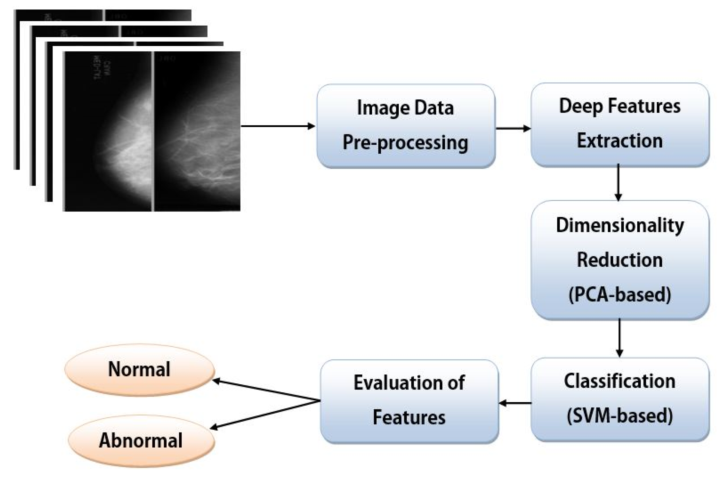
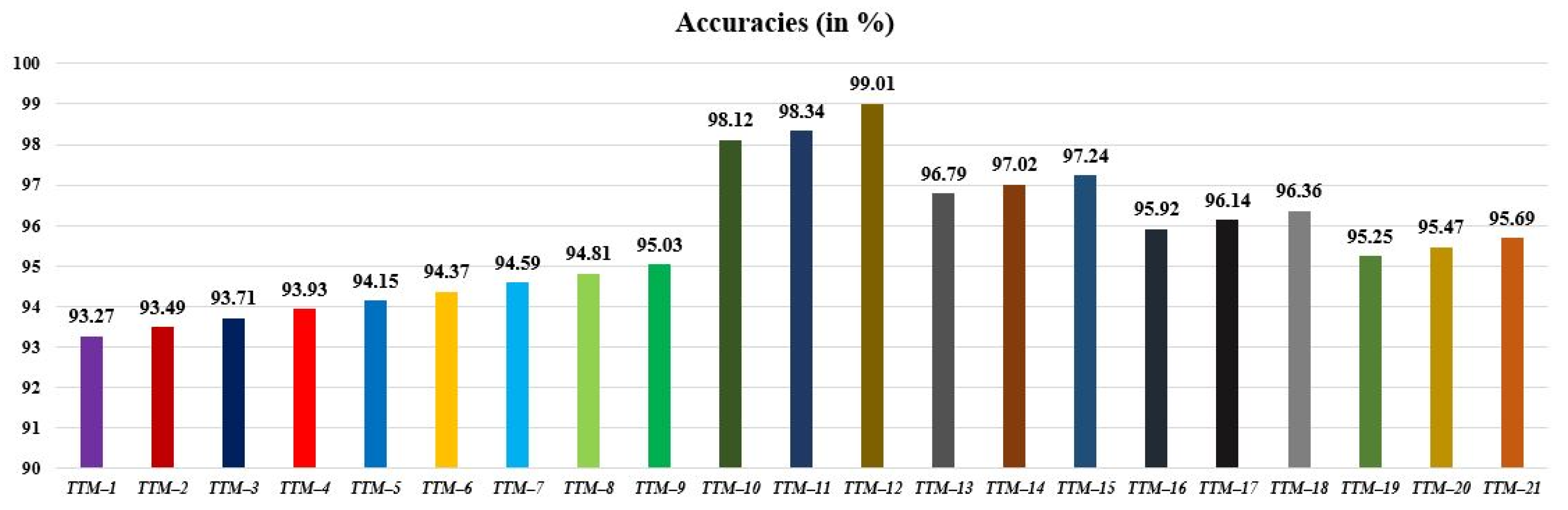
In this work, after image data pre-processing, the deep features were extracted by DCNN with seven TL approaches including InceptionV3, GoogleNet, AlexNet, VGG16, VGG19, ResNet50, and ResNet101. Then, feature dimensions were reduced using PCA and the final features were classified by SVM with three different kernels: linear, polynomial, and RBF. The twenty-one trained TDL models (TTMs) were constructed using these concepts as TTM-1 (InceptionV3 + PCA + SVMLinear), TTM-2 (InceptionV3 + PCA + SVMPolynomial), TTM-3 (InceptionV3 + PCA + SVM-RBF), TTM-4 (GoogleNet + PCA + SVMLinear), TTM-5 (GoogleNet + PCA + SVMPolynomial), TTM-6 (GoogleNet + PCA + SVM-RBF), TTM-7 (AlexNet + PCA + SVMLinear), TTM-8 (AlexNet + PCA + SVMPolynomial), TTM-9 (AlexNet + PCA + SVM-RBF), TTM-10 (VGG16 + PCA + SVMLinear), TTM-11 (VGG16 + PCA + SVMPolynomial), TTM-12 (VGG16 + PCA + SVMRBF), TTM-13 (VGG19 + PCA + SVMLinear), TTM-14 (VGG19 + PCA + SVMPolynomial), TTM-15 (VGG19 + PCA + SVM-RBF), TTM-16 (ResNet50 + PCA + SVMLinear), TTM-17 (ResNet50 + PCA + SVMPolynomial), TTM-18 (ResNet50 + PCA + SVM-RBF), TTM-19 (ResNet101 + PCA + SVMLinear), TTM-20 (ResNet101 + PCA + SVMPolynomial), and TTM-21 (ResNet101 + PCA + SVM-RBF).

Table 4. Findings in % based on various Proposed Approaches.

Proposed TTM Approaches	Findings (in %)
	Acc	MCR	Pre	Sen	Spc	F1S	MCC
TTM–1	93.27	6.73	95.24	96.19	82.33	95.71	80.05
TTM–2	93.49	6.51	95.38	96.33	83.33	95.85	80.71
TTM–3	93.71	6.29	95.52	96.47	83.84	95.99	81.36
TTM–4	93.93	6.07	95.66	96.61	84.34	96.13	82.02
TTM–5	94.15	5.85	95.81	96.75	84.85	96.28	82.67
TTM–6	94.37	5.63	95.94	96.89	85.35	96.42	83.33
TTM–7	94.59	5.41	96.08	97.03	85.86	96.56	83.98
TTM–8	94.81	5.19	96.22	97.18	86.36	96.71	84.64
TTM–9	95.03	4.97	96.36	97.32	86.87	96.84	85.29
TTM–10	98.12	1.88	98.33	99.29	93.81	98.81	94.38
TTM–11	98.34	1.66	98.47	99.44	94.33	98.95	95.04
TTM–12	99.01	0.99	98.89	99.86	95.85	99.37	97.02
TTM–13	96.79	3.21	97.49	98.45	90.86	97.96	90.49
TTM–14	97.02	2.98	97.63	98.59	91.37	98.11	91.15
TTM–15	97.24	2.76	97.77	98.73	91.88	98.25	91.81
TTM–16	95.92	4.08	96.92	97.88	88.89	97.39	87.91
TTM–17	96.14	3.86	97.06	98.02	89.39	97.54	88.57
TTM–18	96.36	3.64	97.21	98.16	89.91	97.68	89.22
TTM–19	95.25	4.75	96.51	97.46	87.37	96.98	85.95
TTM–20	95.47	4.53	96.64	97.61	87.88	97.12	86.59
TTM–21	95.69	4.31	96.78	97.74	88.38	97.26	87.26

displays the obtained findings in % of various proposed TTMs. The TTM-12 had the greatest classification accuracy of 99.01%, as shown in Figure 5, from the observations that outperformed all other twenty hybrid approaches. In addition, this proposed approach also outperformed all others stated in terms of precision, sensitivity, specificity, f1-scores, and MCC.

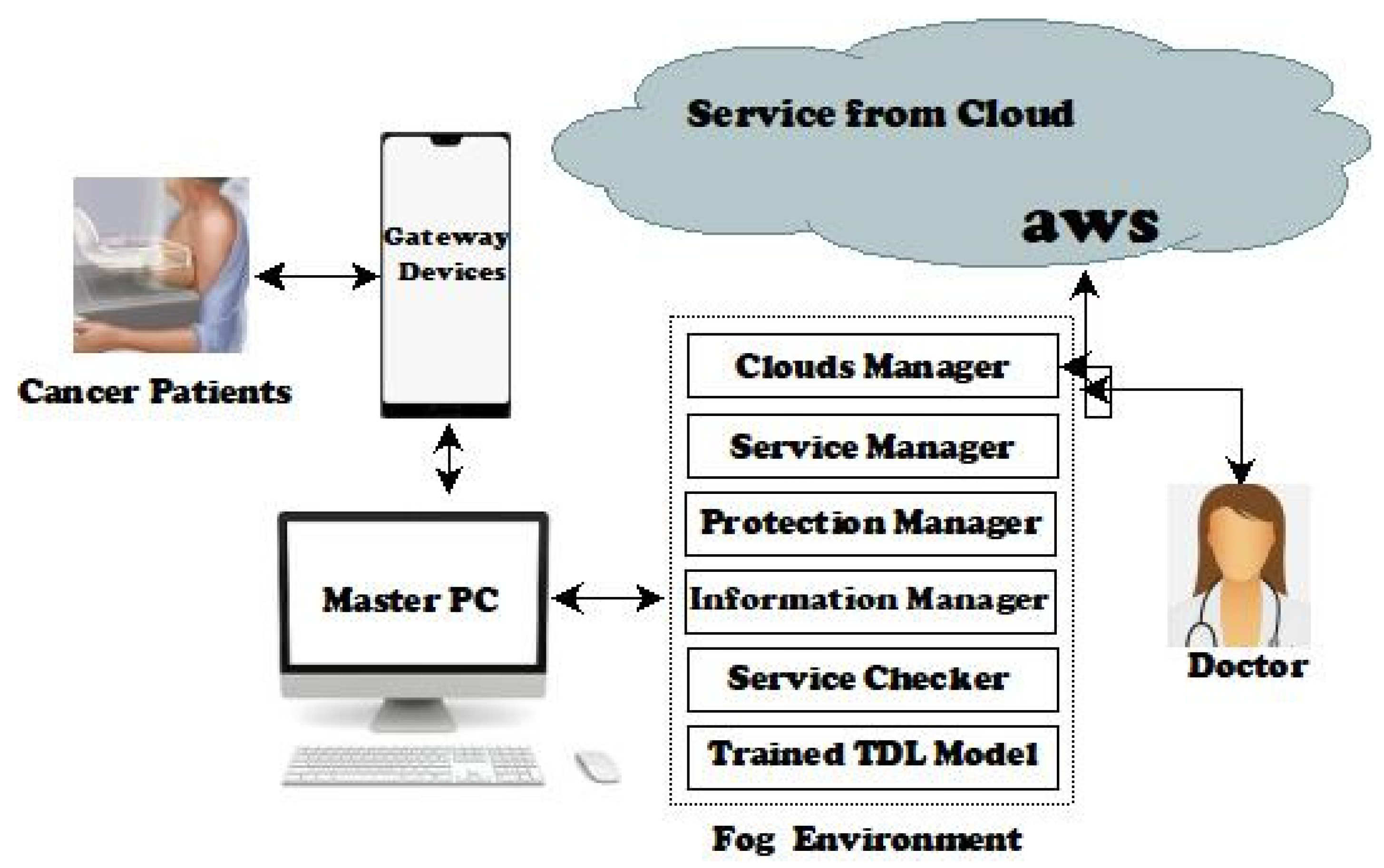
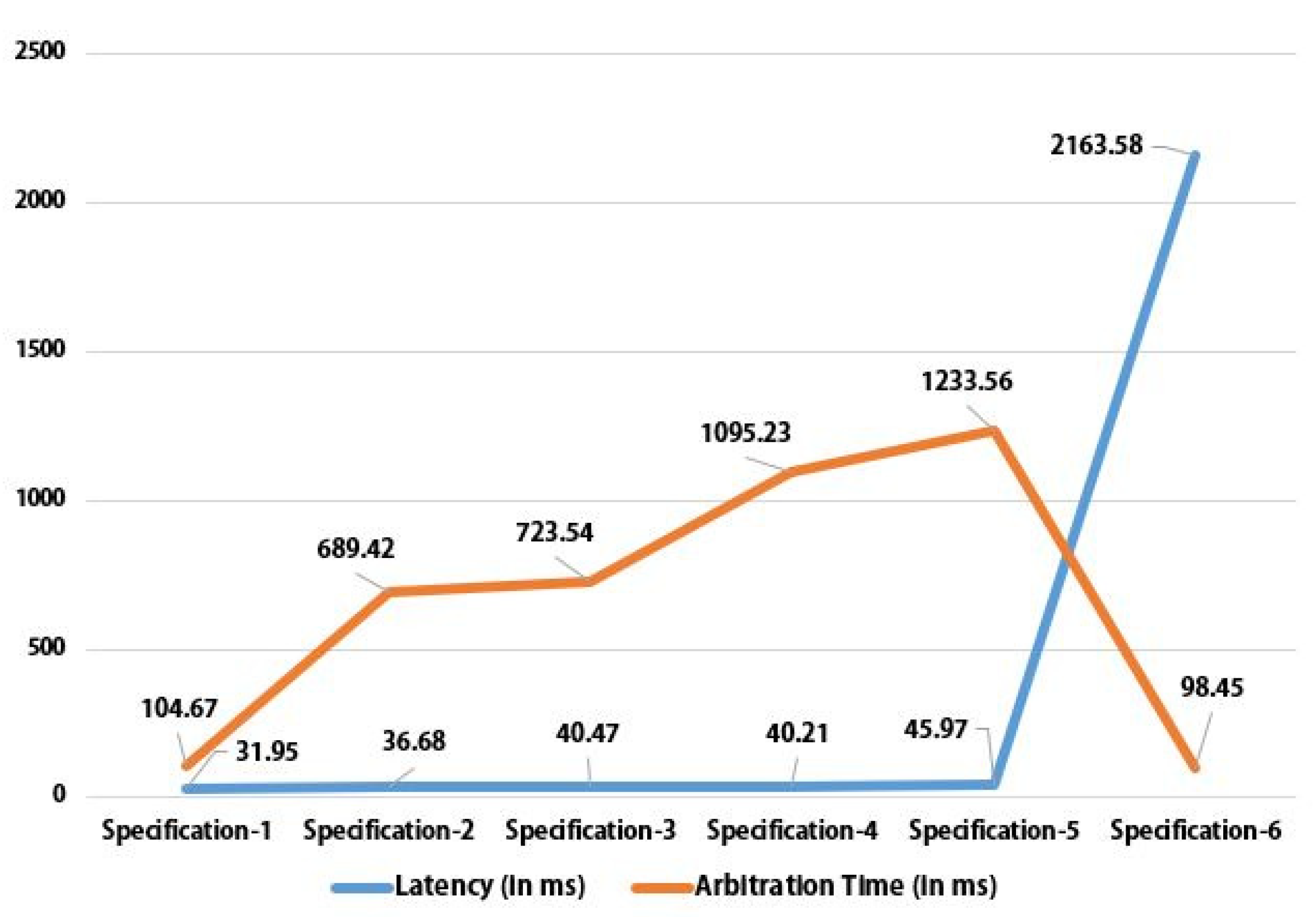
The computing strategy or coordination level utilized by the Fog-enabled IoT application has a big impact on network characteristics. Several network metrics were used to confirm the proposed work for demonstrating the importance of enabling IoT with Fog computing, including latency, arbitration, total processing time, jitter, network, and energy consumption. Specification-1 for Master PC alone, Specification-2 for Master PC with one Fog Worker Node, Specification-3 for Master PC with two Fog Worker Nodes, Specification-4 for Master PC with three Fog Worker Nodes, Specification-5 for Master PC with four Fog Worker Nodes, and Specification-6 for Cloud node only are just a few of the multiple configurations that were employed in this study to evaluate various network metrics.

Data transit time over a network is referred to as latency. It is the time it takes to gather, transport, process, and receive a data packet. Figure 6 illustrates how to compute the difference in latencies by combining transmission time and queuing delay. Because only single-hop data transfers are used for interactions, the latency will be almost identical whether the job is submitted to the MP or the FW Nodes. Fog computing’s principal function of multi-hop data transport outside of the network results in rather significant latency in a Cloud architecture. The “arbitration time” refers to the MP’s reaction time to GTs, depending on how the network is set up. The arbitration time is shown in Figure 6 for varied levels of Fog architectures. Arbitration is less likely to take place when assignments are given directly to Master PC or Cloud nodes. Other times, it takes time to equally distribute the load among the nodes, reducing the arbitration rate. Figure 6 provides a comparative analysis of latency and arbitration time based on various specifications.

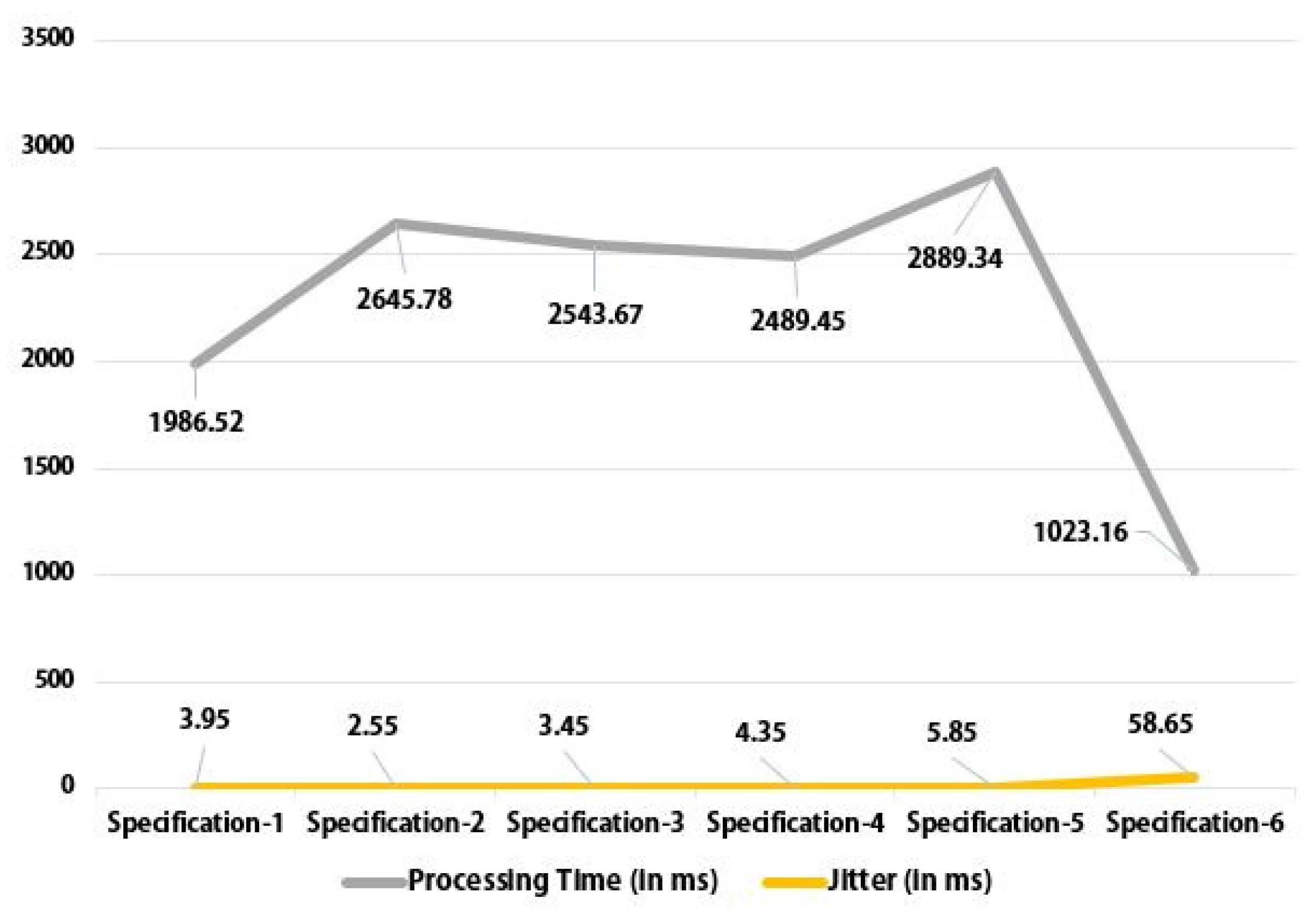
The processing time is the amount of time needed to start, finish, and deliver the work to the users. Figure 7 depicts the processing characteristics under various Fog circumstances. One apparent thing is that employing Cloud communications significantly reduces the overall processing time. The difference in response times between task requests is known as jitter. It is required for many practical applications, including the analysis of data in e-Healthcare systems. The jitter fluctuation for various settings is shown in Figure 7. Because the MP handles resource management, security checking, and arbitration, the jitter is larger in the MP-alone scenario than when tasks are dispersed to FW nodes. When jobs are sent to the Cloud, the jitter is significantly higher. Figure 7 provides a comparative analysis of processing time and jitter based on various specifications.

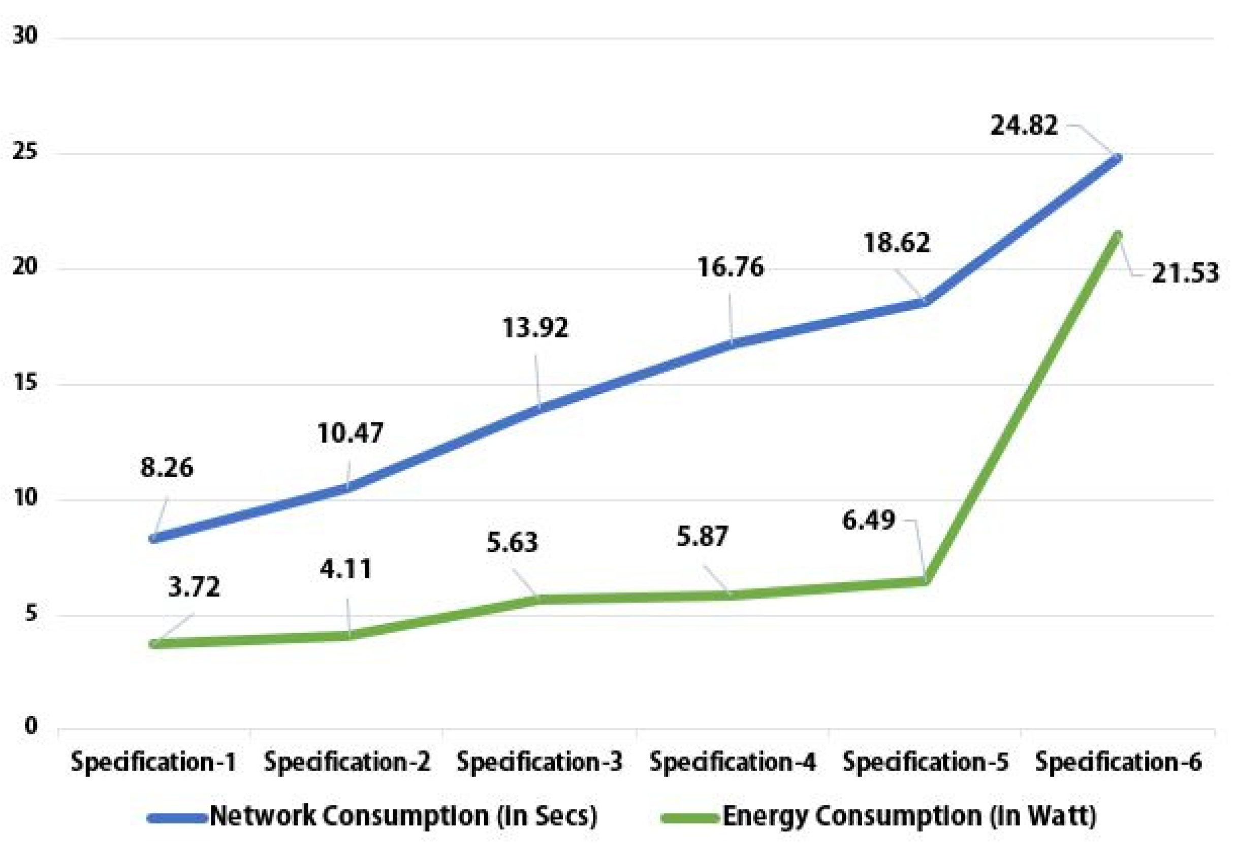
Fog computing uses fewer networks than a Cloud computing system does. The issue has an impact on both the number of FW nodes and the network consumption, which may include MP-alone, FW, or CN nodes. Because the Fog environment, as shown in Figure 8, limits the number of user requests that are sent to the Cloud, network usage time for MP and/or FW nodes is significantly lower than that of CN nodes. The entire amount of energy that the system uses is called energy consumption, which is required by sensors and other system components. As seen in Figure 8, a CN needs a lot more energy than an MP or an FW node. Due to this, CN nodes consume a lot more energy than FW nodes. The proposed work consumes more energy as the quantity of FW nodes increases. Figure 8 provides a comparative analysis of network and energy consumption based on various specifications. Based on the data gathered,

Table 5. Results of various network characteristics as observed using various configurations.

Specifications	Network Parameters
	Latency (in ms)	Arbitration Time (in ms)	Processing Time (in ms)	Jitter (in ms)	Network Utilization (in Secs)	Energy Consumption (in Watt)
Specification-1	31.95	104.67	1986.52	3.95	8.26	3.72
Specification-2	36.68	689.42	2645.78	2.55	10.47	4.11
Specification-3	40.47	723.54	2543.67	3.45	13.92	5.63
Specification-4	40.21	1095.23	2489.45	4.35	16.76	5.87
Specification-5	45.97	1233.56	2889.34	5.85	18.62	6.49
Specification-6	2163.58	98.45	1023.16	58.65	24.82	21.53

displays the averages of the observed results of different network parameters for various specifications.

A scalable infrastructure may add resources while retaining its limits to satisfy changing application needs. Our key concern is whether the system can scale up in quantity as consumers demand it over time, as indicated in Figure 9. The average response time increases as the volume of requests rises, considering specification-5 as the configuration. Additionally, it is highlighted that average response times do not exponentially increase when the number of requests rises, demonstrating the framework’s scalability.

The proposed framework, CanDiag, is compared with some of the current studies that have been taken into consideration in terms of various performance parameters. In

Table 6. A comparison of CanDiag with certain existing state-of-the-art works based on mammogram images.

Work	Methodologies Employed	Dataset(s) Employed	Performance Measures (in %)
			Acc	Pre	Sen	Spc	F1-S	MCR	MCC
[9]	PCA, LDA, SVM	MIAS	97.33	-	-	-	-	-	-
[10]	CNN	mini-MIAS and BCDR	87.00	78.00	90.00	-	84.00	-	-
[11]	CNN	MIAS	90.50	-	89.47	90.71	-	-	-
[12]	FOA, Contourlet, SVM, KNN, NB, and C4.5	MIAS and DDSM	100.00	-	100.00	100.00	-	-	100.00
[14]	CNN, VGG	CBIS-DDSM, BCDR, INBreast, and MIAS	-	-	-	-	94.20	-	-
[16]	CNN	CBIS-DDSM	-	-	-	-	-	-	-
[18]	DCNN, SVM, PCA	MIAS and DDSM	97.90	-	98.00	98.00	96.00	-	-
[19]	CNN, InceptionV2, InceptionV3, ResNet50, VGG-19, VGG-16	MIAS	98.96	97.35	97.83	99.13	97.66	-	-
[20]	CNN, SVM, RF	Dataset from Kaggle	99.65	-	-	-	-	-	-
[21]	DCNN, VGG-16, VGG-19	DDSM and PINUM	90.00	89.00	99.00	83.00	85.00	-	-
[22]	ResNet-164, AlexNet, InceptionV3, VGG-19	Dataset from TCIA	97.00	-	-	-	98.00	-	-
[24]	DLCN, SGO, BPNN	mini-MIAS and DDSM	98.50	-	98.46	99.08	98.91	-	-
[25]	AlexNet, LS-SVM, KNN, RF, and NB	MIAS	98.00	96.00	97.00	97.00	97.50	-	-
Proposed Work	DCNN, GoogleNet, ResNet50, ResNet101 InceptionV3, AlexNet, VGG16, VGG19, PCA, SVM	MIAS	99.01	98.89	99.86	95.85	99.37	0.99	97.02

, the proposed work is compared with some state-of-the-art works based on DL and TL approaches and mammogram imaging datasets considering the comparison parameters as methodologies, datasets employed, and the performance parameters including accuracy, precision, sensitivity, specificity, f1-score, MCR, and MCC. Based on the experimental outcomes, it can be concluded that this proposed work outperforms in some cases and also falls short in some cases.

The proposed framework, CanDiag, was also compared with previous studies on performance and network parameters concerning cancer diseases with Fog computing concepts. The network’s consumption, energy consumption, scalability, etc., were examined for the first time, showing the work’s novelty.

Table 7. A contrast of CanDiag with certain state-of-the-art works based on approaches and parameters of cancer diagnosis with Fog computing.

Author	Concepts Employed					Performance Parameters Employed							Network Parameters Employed
	IoT	CC	FC	ML/DL	TL	Acc	MCR	Pre	Sen	Spc	F1S	MCC	LT	AT	PT	JT	EC	NC	SB
[13]	1	1	1	-	-	1	-	-	-	-	-	-	1	-	-	-	-	-	-
[15]	1	1	1	1	-	1	-	-	-	-	-	-	1	-	1	-	-	-	-
[17]	1	1	1	1	-	1	-	1	1	-	-	-	-	-	-	-	-	-	-
[23]	1	1	1	1	-	1	-	-	-	-	-	-	1	-	1	-	-	1	-
[26]	1	1	1	1	1	1	1	1	1	1	1	-	-	-	-	-	-	-	-
Proposed Work	1	1	1	1	1	1	1	1	1	1	1	1	1	1	1	1	1	1	1

compares DiaFog with numerous key outcomes from this research. Table 7 abbreviates the Presence of Concepts (1), Jitter (JT), Energy Consumption (EC), Processing Time (PT), Network Consumption (NC), Arbitration Time (AT), Latency (LT), and Scalability (SB).

6. Conclusions and Future Scope

Fog computing with IoT applications has become more crucial to make people’s lives easier and better. Given the severity of the breast cancer situation, allowing the patient to use IoT applications for remote self-diagnosis is beneficial. Formal IoT implications, however, simply call for cloud infrastructures for instantaneous data storing, scrutiny, etc., which have several concerns including latency, network, and energy consumption, security and privacy, etc. To solve these problems, Fog computing should be combined with IoT and Cloud computing. This study suggests using numerous TDL techniques along with PCA and SVM in a Fog-enabled system for instantaneous breast cancer patient diagnosis. A dataset made up of mammography images that were collected from the MIAS warehouse was used to create this TTM model. Various performance and network parameters of this study are investigated. With an accuracy, MCR, precision, sensitivity, specificity, f1-scores, and MCC of 99.01%, 0.99%, 98.89%, 99.86%, 95.85%, 99.37%, and 97.02%, respectively, the research on the dataset of mammography images categorized as normal and abnormal outperformed some earlier studies.

This proposed work can be beneficial from the instantaneous remote self-diagnosis of individuals relating to breast cancer diseases. However, there are some limitations to this work, including the cost and difficulty of the entire development and execution of the proposed work that can be included in future works as summarized and listed: (i) Applying these frameworks on various Image-based datasets having multi-class variables; (ii) Inclusion of LDA as an alternative to PCA for dimensionality reduction; (iii) Expansions of this study could be utilized to treat a variety of other chronic illnesses; (iv) Alternative Cloud computing platforms, including Edge computing, Mist computing, and Surge computing, should also be employed to enhance the architecture provided; and (v) The challenge of a single network platform is another area that we should focus on in the future.

References

1. Arnold, M.; Morgan, E.; Rumgay, H.; Mafra, A.; Singh, D.; Laversanne, M.; Vignat, J.; Gralow, J.R.; Cardoso, F.; Siesling, S.; et al. Current and future burden of breast cancer: Global statistics for 2040. Breast 2022, 66, 15–23. [Google Scholar] [CrossRef] [PubMed]
2. Pati, A.; Parhi, M.; Pattanayak, B.K. IABCP: An Integrated Approach for Breast Cancer Prediction. In Proceedings of the 2022 2nd Odisha International Conference on Electrical Power Engineering, Communication and Computing Technology (ODICON), Bhubaneswar, India, 11–12 November 2022; pp. 1–5. [Google Scholar]
3. Kshirsagar, P.R.; Manoharan, H.; Shitharth, S.; Alshareef, A.M.; Albishry, N.; Balachandran, P.K. Deep learning approaches for prognosis of automated skin disease. Life 2022, 12, 426. [Google Scholar] [CrossRef] [PubMed]
4. Saxena, S.; Shukla, S.; Gyanchandani, M. Breast cancer histopathology image classification using kernelized weighted extreme learning machine. Int. J. Imaging Syst. Technol. 2021, 31, 168–179. [Google Scholar] [CrossRef]
5. Goen, A.; Singhal, A. Classification of Breast Cancer Histopathology Image using Deep Learning Neural Network. Int. J. Eng. Res. Appl. 2021, 11, 59–65. [Google Scholar]
6. Pati, A.; Parhi, M.; Pattanayak, B.K.; Singh, D.; Samanta, D.; Banerjee, A.; Biring, S.; Dalapati, G.K. Diagnose Diabetic Mellitus Illness Based on IoT Smart Architecture. Wirel. Commun. Mob. Comput. 2022, 2022, 7268571. [Google Scholar] [CrossRef]
7. Mutlag, A.A.; Abd Ghani, M.K.; Mohammed, M.A.; Lakhan, A.; Mohd, O.; Abdulkareem, K.H.; Garcia-Zapirain, B. Multi-Agent Systems in Fog–Cloud Computing for Critical Healthcare Task Management Model (CHTM) Used for ECG Monitoring. Sensors 2021, 21, 6923. [Google Scholar] [CrossRef]
8. Pati, A.; Parhi, M.; Pattanayak, B.K. HeartFog: Fog Computing Enabled Ensemble Deep Learning Framework for Automatic Heart Disease Diagnosis. In Intelligent and Cloud Computing; Springer: Singapore, 2022; pp. 39–53. [Google Scholar]
9. Khan, S.; Hussain, M.; Aboalsamh, H.; Bebis, G. A comparison of different Gabor feature extraction approaches for mass classification in mammography. Multimed. Tools Appl. 2017, 76, 33–57. [Google Scholar] [CrossRef]
10. Hepsag, P.U.; Ŏzel, S.A.; Yazıcı, A. Using deep learning for mammography classification. In Proceedings of the 2017 International Conference on Computer Science and Engineering (UBMK), Antalya, Turkey, 5–8 October 2017; pp. 418–423. [Google Scholar]
11. Ting, F.F.; Tan, Y.J.; Sim, K.S. Convolutional neural network improvement for breast cancer classification. Expert Syst. Appl. 2019, 120, 103–115. [Google Scholar] [CrossRef]
12. Mohanty, F.; Rup, S.; Dash, B.; Majhi, B.; Swamy, M.N.S. Mammogram classification using contourlet features with forest optimization-based feature selection approach. Multimed. Tools Appl. 2019, 78, 12805–12834. [Google Scholar] [CrossRef]
13. Abd-Elmegid, L.A. A Proposed Architecture for Predicting Breast Cancer using Fog Computing. Communications 2019, 7, 32–35. [Google Scholar]
14. Chougrad, H.; Zouaki, H.; Alheyane, O. Multi-label transfer learning for the early diagnosis of breast cancer. Neurocomputing 2020, 392, 168–180. [Google Scholar] [CrossRef]
15. Xu, J.; Liu, H.; Shao, W.; Deng, K. Quantitative 3-D shape features based tumor identification in the fog computing architecture. J. Ambient. Intell. Humaniz. Comput. 2019, 10, 2987–2997. [Google Scholar] [CrossRef]
16. Zhu, G.; Fu, J.; Dong, J. Low-Dose Mammography via Deep Learning. J. Phys. Conf. Ser. 2020, 1626, 012110. [Google Scholar] [CrossRef]
17. Rajan, J.P.; Rajan, S.E.; Martis, R.J.; Panigrahi, B.K. Fog computing employed computer-aided cancer classification system using deep neural network in internet of things-based healthcare system. J. Med. Syst. 2020, 44, 34. [Google Scholar] [CrossRef] [PubMed]
18. Ragab, D.A.; Attallah, O.; Sharkas, M.; Ren, J.; Marshall, S. A framework for breast cancer classification using multi-DCNNs. Comput. Biol. Med. 2021, 131, 104245. [Google Scholar] [CrossRef]
19. Saber, A.; Sakr, M.; Abo-Seida, O.M.; Keshk, A.; Chen, H. A novel deep-learning model for automatic detection and classification of breast cancer using the transfer-learning technique. IEEE Access 2021, 9, 71194–71209. [Google Scholar] [CrossRef]
20. Allugunti, V.R. Breast cancer detection based on thermographic images using machine learning and deep learning algorithms. Int. J. Eng. Comput. Sci. 2022, 4, 49–56. [Google Scholar]
21. Rehman, K.U.; Li, J.; Pei, Y.; Yasin, A.; Ali, S.; Mahmood, T. Computer vision-based microcalcification detection in digital mammograms using fully connected depth-wise separable convolutional neural network. Sensors 2021, 21, 4854. [Google Scholar] [CrossRef]
22. Canatalay, P.J.; Ucan, O.N.; Zontul, M. Diagnosis of breast cancer from X-ray images using deep learning methods. PONTE Int. J. Sci. Res. 2021, 77, 2505. [Google Scholar] [CrossRef]
23. Zhu, X.; Zhu, Y.; Li, L.; Pan, S.; Tariq, M.U.; Jan, M.A. IoHT-enabled gliomas disease management using fog Computing for sustainable societies. Sustain. Cities Soc. 2021, 74, 103215. [Google Scholar] [CrossRef]
24. Kavitha, T.; Mathai, P.P.; Karthikeyan, C.; Ashok, M.; Kohar, R.; Avanija, J.; Neelakandan, S. Deep learning-based capsule neural network model for breast cancer diagnosis using mammogram images. Interdiscip. Sci. Comput. Life Sci. 2022, 14, 113–129. [Google Scholar] [CrossRef] [PubMed]
25. Jasti, V.; Zamani, A.S.; Arumugam, K.; Naved, M.; Pallathadka, H.; Sammy, F.; Raghuvanshi, A.; Kaliyaperumal, K. Computational technique based on machine learning and image processing for medical image analysis of breast cancer diagnosis. Secur. Commun. Netw. 2022, 2022, 1918379. [Google Scholar] [CrossRef]
26. Nasir, M.U.; Khan, S.; Mehmood, S.; Khan, M.A.; Rahman, A.U.; Hwang, S.O. IoMT-Based Osteosarcoma Cancer Detection in Histopathology Images Using Transfer Learning Empowered with Blockchain, Fog Computing, and Edge Computing. Sensors 2022, 22, 5444. [Google Scholar] [CrossRef] [PubMed]
27. Suckling, J.; Parker, J.; Dance, D.; Astley, S.; Al, E. The mammographic image analysis society digital mammogram database. Exerpta Medica. Int. Congr. Ser. 1994, 1069, 375–378. [Google Scholar]
28. Khan, R.U.; Zhang, X.; Kumar, R. Analysis of ResNet and GoogleNet models for malware detection. J. Comput. Virol. Hacking Tech. 2019, 15, 29–37. [Google Scholar] [CrossRef]
29. Theckedath, D.; Sedamkar, R.R. Detecting affect states using VGG16, ResNet50 and SE-ResNet50 networks. SN Comput. Sci. 2020, 1, 1–7. [Google Scholar]
30. Ullah, A.; Elahi, H.; Sun, Z.; Khatoon, A.; Ahmad, I. Comparative analysis of AlexNet, ResNet18 and SqueezeNet with diverse modification and arduous implementation. Arab. J. Sci. Eng. 2022, 47, 2397–2417. [Google Scholar] [CrossRef]
31. Selvaraj, T.; Rengaraj, R.; Venkatakrishnan, G.; Soundararajan, S.; Natarajan, K.; Balachandran, P.; David, P.; Selvarajan, S. Environmental Fault Diagnosis of Solar Panels Using Solar Thermal Images in Multiple Convolutional Neural Networks. Int. Trans. Electr. Energy Syst. 2022, 2022, 2872925. [Google Scholar] [CrossRef]
32. Yu, Y.; Samali, B.; Rashidi, M.; Mohammadi, M.; Nguyen, T.N.; Zhang, G. Vision-based concrete crack detection using a hybrid framework considering noise effect. J. Build. Eng. 2022, 61, 105246. [Google Scholar] [CrossRef]
33. Sahu, B.; Panigrahi, A.; Rout, S.K.; Pati, A. Hybrid Multiple Filter Embedded Political Optimizer for Feature Selection. In Proceedings of the 2022 International Conference on Intelligent Controller and Computing for Smart Power (ICICCSP), Hyderabad, India, 21–23 July 2022; pp. 1–6. [Google Scholar]
34. Yu, Y.; Liang, S.; Samali, B.; Nguyen, T.N.; Zhai, C.; Li, J.; Xie, X. Torsional capacity evaluation of RC beams using an improved bird swarm algorithm optimised 2D convolutional neural network. Eng. Struct. 2022, 273, 115066. [Google Scholar] [CrossRef]
35. Pati, A.; Parhi, M.; Pattanayak, B.K. IHDPM: An integrated heart disease prediction model for heart disease prediction. Int. J. Med. Eng. Inform. 2022, 14, 564–577. [Google Scholar]
36. Pati, A.; Parhi, M.; Pattanayak, B.K. A review on prediction of diabetes using machine learning and data mining classification techniques. Int. J. Biomed. Eng. Technol. 2023, 41, 83–109. [Google Scholar] [CrossRef]
37. Gupta, H.; Vahid Dastjerdi, A.; Ghosh, S.K.; Buyya, R. iFogSim: A toolkit for modeling and simulation of resource management techniques in the Internet of Things, Edge and Fog computing environments. Softw. Pract. Exp. 2017, 47, 1275–1296. [Google Scholar] [CrossRef]
38. Tuli, S.; Mahmud, R.; Tuli, S.; Buyya, R. FogBus: A Blockchain-based Lightweight Framework for Edge and Fog Computing. J. Syst. Softw. 2019, 154, 22–36. [Google Scholar] [CrossRef]
39. Narula, S.; Jain, A. Cloud computing security: Amazon web service. In Proceedings of the 2015 Fifth International Conference on Advanced Computing & Communication Technologies, Haryana, India, 21–22 February 2015; pp. 501–505. [Google Scholar] [CrossRef]
40. Vecchiola, C.; Chu, X.; Buyya, R. Aneka: A software platform for .NET-based cloud computing. High Speed Large Scale Sci. Comput. 2009, 18, 267–295. [Google Scholar]
41. Pati, A.; Parhi, M.; Alnabhan, M.; Pattanayak, B.K.; Habboush, A.K.; Al Nawayseh, M.K. An IoT-Fog-Cloud Integrated Framework for Real-Time Remote Cardiovascular Disease Diagnosis. Informatics 2023, 10, 21. [Google Scholar] [CrossRef]
42. Parhi, M.; Roul, A.; Ghosh, B.; Pati, A. Ioats: An intelligent online attendance tracking system based on facial recognition and edge computing. Int. J. Intell. Syst. Appl. Eng. 2022, 10, 252–259. [Google Scholar]
43. Sahu, B.; Panigrahi, A.; Mohanty, S.; Sobhan, S. A hybrid cancer classification based on SVM optimized by PSO and reverse firefly algorithm. Int. J. Control Autom. 2020, 13, 506–517. [Google Scholar]
Figure 1. Fog–Cloud-based distributions to IoT Healthcare systems.
Designs 07 00057 g001
Figure 2. Samples from MIAS Dataset (First two are examples of Abnormal and the last one belongs to the Normal Class).
Designs 07 00057 g002
Figure 3. Block Diagram of the Proposed Trained Model.
Designs 07 00057 g003
Figure 4. The Architecture of the Proposed CanDiag Framework.
Designs 07 00057 g004
Figure 5. Comparative analysis of various proposed TTM approaches based on their achieved accuracies in %.
Designs 07 00057 g005
Figure 6. Latency vs. Arbitration time based on various specifications.
Designs 07 00057 g006
Figure 7. Processing time vs. Jitter based on various specifications.
Designs 07 00057 g007
Figure 8. Network vs. Energy consumption based on various specifications.
Designs 07 00057 g008
Figure 9. The average response duration is given to the volume of requests.
Designs 07 00057 g009