Article

CFD Investigation of Ventilation Strategies to Remove Contaminants from a Hospital Room

1
Wind Energy Research Laboratory, The University of Quebec at Rimouski, Rimouski, QC G5L 3A1, Canada
2
École de Technologie Supérieure, Montréal, QC H3C 1K3, Canada
*
Author to whom correspondence should be addressed.
Submission received: 30 November 2022 / Revised: 26 December 2022 / Accepted: 29 December 2022 / Published: 4 January 2023
(This article belongs to the Topic Building Energy and Environment)

Abstract

:
The primary requirement in designing air conditioning systems in healthcare facilities is eliminating contaminants. It is considered one of the crucial health elements in building design, particularly in the presence of many airborne diseases such as COVID-19. The purpose of this numerical research is to simulate various ventilation designs for a hospital room model by taking into account results obtained by previous researchers. Four designs with three airflows, 9, 12, and 15 ACH (Air Change per Hour), are applied to explore the capacity of the ventilation system to remove contaminants. The objective is to determine the influence of airflow and the diffuser location distribution on the pollutants elimination represented by carbon dioxide. The Reynold Averaged Navier–Stokes (RANS) equations and the k-ε turbulence model were used as the underlying mathematical model for the airflow. In addition, boundary conditions were extracted from ASHRAE (American Society of Heating, Refrigeration, and Air-Conditioning Engineers Society) ventilation publications and relevant literature. Contrary to what was expected, this study’s results demonstrated that increased ventilation alone does not always improve air distribution or remove more contaminants. In addition, pollutant removal was significantly affected by the outlet’s location.

1. Introduction

The coronavirus pandemic has resulted in more than 15 million infections and over 619,000 deaths worldwide in 2020. The regions most affected by the pandemic are Asia, particularly China, Europe, the United States, South America, and Mexico. Severe acute respiratory syndrome (SARS-CoV-2) can spread over long distances in the air. Therefore, airborne transmission played a significant role in the rapid propagation of the epidemic [1]. Given the rapid spread of the disease, hospitals are compelled to treat patients in isolation. When an infected individual sneezes or coughs, microscopic particles are disseminated throughout the environment. If another person inhales these particles, they may become sick. Therefore, airborne infectious diseases can rapidly spread in an inadequately ventilated isolation room. Rooms with a proper ventilation system will be free of infectious airborne particles, such as viruses, bacteria, or microorganisms [2,3].
During the ventilation system operation, the occupants’ attention is focused on thermal comfort because the sensation of thermal comfort is immediate and thermal discomfort cannot be tolerated. However, poor air quality is hard to notice, so the occupants’ response takes longer [4]. Therefore, efficient ventilation and adequate indoor air quality (IAQ) are essential for human health, well-being, and productivity. For instance, a good IAQ effectively removes indoor pollutants and introduces an adequate quantity of fresh outdoor air for occupants [5]. Several indicators assess ventilation efficiency.
Contaminant removal efficiency (CRE) and air exchange efficiency (ACE) are indicators regularly used as they can be easily measured both in a laboratory and in the field and can be applied to all ventilation methods. In addition, they are generic, and almost all other indicators are extensions of them. For example, CRE is an indicator of the pollution level in a room that depends not only on the airflow pattern but also on the characteristics of pollutant sources, such as density, area, and position [4].
IAQ can be assessed in terms of the concentration of gaseous ingredients. Many gaseous ingredients such as volatile organic compounds (VOCs), formaldehyde, nitrogen oxides, sulfur oxide, carbon dioxide, carbon monoxide, particulates, and infectious pollutants often degrade indoor air quality. The high concentration of these pollutants leads to serious health effects and inconvenience for patients. However, pollutants other than carbon dioxide are usually recorded as sufficiently below the standard limit [6]. In addition, the carbon dioxide concentration depends on the number of humans inside an occupied space. Therefore, carbon dioxide concentration is widely used as an indicator of IAQ.
No sole ventilation design solution can solve all the airborne transferable particle concentration problems and consistently be cost-effective. Therefore, ventilation designers must always consider the cost of installing and operating their systems and need effective control strategies for air systems to make a feasible design [7]. Therefore, various healthcare facility ventilation designs provide a minimum ventilation equivalent to 12 ACH (Air Change per Hour) for isolation rooms [8]. According to [9], the transmission of air pollutants can spread disease to healthcare workers and patients.
The pressure value of the air inside a hospital room should be checked and adjusted correctly accordingly to its usage. For example, if the room is host to a transmissible disease, the room’s pressure is lowered to prevent particles from leaking out of the room; if the room is used for an operation, the room’s pressure is increased to prevent particles from entering so the space can be kept sterile [10]. Therefore, for the systems serving Airborne Infection Isolation Rooms (AIIR), negative air pressure must be designed relative to adjacent rooms or hallways. However, an AIIR plan with negative pressure involves a complex decision-making process [11].
Several studies have noted an interdependence between ventilation and health, but the actual relationship and attributable mechanisms remain unclear. In addition, the data was insufficient to define minimum ventilation standards to control the prevalence of airborne disease in any setting. Consequently, it revealed the uncertainty about the connection between ventilation and health [12].
Researchers have examined how different vent placements affect the flow and heat transmission characteristics inside an enclosed system with a volumetric heat source. Three aspect ratios H/W = 1, 2, 3, and three Rah = 103, 104, 105, have been examined together with two global factors, the mass flow rate and Nu. The conclusion is that the position of the vent should minimize the dead zone size. In addition, the transfer properties of the system would improve if the dead zones were reduced [13].
The airflow direction depends on the room pressure and the inlet/outlet distribution through the space. Accordingly, a cautious and intentional ventilation device can be more effective in containing and removing airborne contaminants [12]. Unfortunately, the literature does not provide enough indication of the location of outlets and inlets. For example, it does not limit the maximum and minimum distances between the two openings [14]. As per ASHRAE standards, space air diffusion has defined some particular rules, trying to guide the designers toward the best solution. For example, it mentions that the outlet diffuser should be located on the side of the room away from the supply diffuser to reduce short-circuiting of supplied air [14].
Using computational fluid dynamics modeling and field measurement, a comparison of the efficiency of three ventilation systems has been made in a study by Cho [11]. The research aimed to protect medical personnel from inhaling patients’ respiratory droplets of sputum in an isolation room provided with negative pressure. A new ventilation approach for isolation rooms is proposed based on empirical data and simulated findings from three ventilation systems that have been effective in removing pollutants. The results show that ventilation systems using the “low-level extraction” method are superior for removing contaminants from the breathing zone.
The air change rate and pollutant removal efficiency were used to assess AIIR ventilation performance in three Finnish hospitals [14,15]. The results showed that the AIIR’s and anteroom’s high ventilation rates (4–24) ACH were insufficient to stop the spread of infectious microorganisms due to improper airflow.
Researchers at the University of Cordoba [16] conducted an experimental and numerical study to assess ventilation at three different rates of air change of 6, 9, and 12 ACH in the transport of pollutants to a patient (P) lying in a hospital bed to a healthcare worker (HCW) standing beside the bed. They found that increasing ACH cannot reduce exposure and, in some circumstances, may increase it.
Another numerical study [17] aimed to recognize the role of ventilation in preventing and controlling infection in general hospital wards and obtain a simple design, cost-effective ventilation system to reduce infection. The study’s results revealed that rearranging the air return diffuser position and increasing the aeration rate to 12 ACH kept the ventilation under control and enhanced its ability to reduce the risk of transmitting diseases to public wards.
Experimental and numerical tests have been performed [18] in a hospital to monitor the circulation and removal of inhalable aerosols (0.5–10 μ m ) based on the ventilation rate in the isolation room. It was found that increased ventilation from 2.5 to 5.5 ACH resulted in reducing aerosol concentrations by only 30%. Higher ventilation rates were not relatively effective in reducing the concentration of pollutants.
A numerical computational fluid dynamics (CFD) approach is applied by Lu et al. [19] to investigate if the representation of CO2 could be achieved and explore contaminant distribution in a two-bed hospital ward with two patients and one healthcare worker under different types of ventilation. For simulating the exhaled and coughed contaminants by patients with different postures, a tracer gas (CO2) is applied. The results demonstrate that stratum ventilation minimizes the exposure risk of healthcare workers in hospital wards. Furthermore, under stratum ventilation, the contaminant concentration in the breathing zone at 1.3–1.7 m above the floor is lower, and the contaminant removal effectiveness is comparably higher.
The primary limitations and solutions in the epidemic era have been assessed by Fan et al. [20]. They reviewed the most up-to-date scientific literature on indoor ventilation modes and manuals from different countries, identifying characteristics of different ventilation modes and evaluating effects in different application occasions. In addition, they studied which virus spread regulations and operating modes, including non-uniform and unstable ones, demonstrated the best performance for air quality.
To determine the importance of the air outlet near the patient, Borro et al. [1] investigated the role of HVAC systems in spreading infection through CFD simulation cough at Bambino Gesu Children’s Hospital in the Vatican State. In addition, the potential role of exhaust ventilation systems placed over the mouth of a coughing patient was also assessed. Despite doubling the airflow in the HVAC system providing a significant reduction in the concentration of airborne pollutants, it also results in a significant increase in turbulent air movement, which gives the droplets and air pollutants a spread of increased and faster long-range in the room. However, the presence of the local exhaust ventilation (LEV) unit above the patient’s face illustrates a very high capacity to reduce droplets and polluted air in the room, guaranteeing the total absence of exposure to infection risks for the patient.
Another study [21] examined the ventilation system’s performance in a standard hospital room using SolidWorks flow simulation software. Achieving indoor air quality (IAQ) depends on many factors, including removing pollutants. Therefore, CRE greater than one is strongly recommended for the optimal ventilation system. The simulation gives a CRE of 1.23 for exhaled air, which means that the ventilation system is reasonably efficient in removing polluted air, although the study result was satisfactory. However, the results obtained through this study are not blindly applicable to hot and humid countries.
The primary goal of this research is to conduct a numerical study of several ventilation system strategies for a hospital isolation room. This study focuses on determining the optimum strategy to protect healthcare workers from being inoculated, eliminate infectious sources, or reduce their spread. The findings were explored in detail via the Local Air Quality Index (LAQI) by demonstrating the efficiency of the ventilation to eliminate contaminants at each point in the space. In addition, we present the trace study to illustrate the steady-state diffusion of the contaminants and CRE to demonstrate the efficiency with which the ventilation system eliminates them.

2. Methodology

CFD is the most advanced building simulation method and uses Navier–Stokes equations to solve the flow field in the fluid domain inside the building [22,23].

2.1. Governing Equations

2.1.1. Turbulence Model

Reynolds number is the product of representative velocity and length scales divided by kinematic viscosity and characterizes laminar and turbulent flows. Most of the fluid flows encountered in engineering practice are considered turbulent, so flow simulations were mainly developed to simulate and study turbulent flows. Average Favre-Navier–Stokes equations are used to predict turbulent flows, in which the effects of time-averaged flow turbulence on flow parameters are considered.
Previous publications have established that the Reynolds-averaged-Navier–Stokes approach is adequate for modeling airflow in closed spaces. Two additional partial differential equations associated with the k-ε turbulence model complete mathematical closure [12,23].
The general laws of mass, angular momentum, and energy conservation can be written in a cartesian frame rotating at an angular speed around an axis passing through the origin of the frame in the following conservation form (Solidworks Flow Simulation). The subscripts, unless stated otherwise, are used to denote summation over the three coordinate directions, x, y, and z, associated with i = 1, i = 2, and i = 3, respectively [24,25]:
ρ t + x i ( ρ u i ) = 0
ρ u i t + x i ( ρ u i u j ) + p x i = x i ( τ i j + τ i j R ) + S i ; i = 1 , 2 , 3
ρ H t + ρ u i H x i = x i ( u j ( τ i j + τ i j R ) + q i ) + p t τ i j R u i x j + ρ ε + S i u i + Q H ,
H = h + u 2 2 + 5 3 k Ω 2 r 2 2 m h m 0 y m ,
Here, u is the fluid velocity, ρ is the fluid density, S i is a mass-distributed external force per unit mass due to a porous media resistance ( S i p o r o u s ) , a buoyancy ( S i g r a v i t y = ρ g i ) , where g i is the gravitational acceleration component along the i-th coordinate direction, and the coordinate system’s rotation ( S i r o t a t i o n ) , i.e., S i = ( S i p o r o u s + S i g r a v i t y + S i r o t a t i o n ) .   h is the thermal enthalpy, Q H is a heat source or sink per unit volume, τ i j is the viscous shear stress tensor, q i   is the diffusive heat flux, Ω is the angular velocity of the coordinate system in rotation, r is the distance between a point and the axis of rotation in the frame of rotation, k is the kinetic energy of the turbulence, h m 0 is an individual thermal enthalpy of the m-th component of the mixture, y m   is a concentration of the m-th component of the mixture. Subscripts are used to indicate grouping across the three coordinate directions. In our study, there is no rotation of the flow domain and no porous media resistance. Therefore, those terms are set to zero in the simulations.
The viscous shear tensor for Newtonian fluids is defined as:
τ i j = μ ( u i x j + u j x i 2 3 δ i j u k x k )
The Reynolds-stress tensor as the following Boussinesq assumption has the following form:
τ i j R = μ t ( u i x j + u j x i 2 3 δ i j u k x k ) 2 3 ρ k δ i j
Here, is δ i j the Kronecker delta function (it is equal to unity when i = j , and zero otherwise), μ is the dynamic viscosity parameter, μ t   is the turbulent eddy viscosity coefficient and k is the turbulent kinetic energy. Note that μ t and k are zero for laminar flows. Within k- ε turbulence model, μ t   is computed using the turbulent dissipation ε and the turbulent kinetic energy k .
μ t = f μ C μ ρ k 2 ε
Here f μ is a turbulent viscosity factor. It is defined by the expression
f μ = [ 1 exp ( 0.0165 R y ) ] 2 × ( 1 + 20.5 R T ) ,
where: R T = ρ k 2 μ ε   , R y = ρ k y μ . with y the distance to the wall. This function makes it possible to take into account the laminar-turbulent transition. Two additional transport equations are used to describe turbulent kinetic energy and dissipation,
ρ k t + x i ( ρ u i k ) = x i ( ( μ + μ t σ k ) k x i ) + S k   ,
ρ ε t + x i ( ρ u i ε ) = x i ( ( μ + μ t σ ε ) ε x i ) + S ε   ,
Here, the source terms S k and S ε   are given by:
S k   = τ i j R u i x j ρ ε + μ t P B
S ε   = C ε 1 ε k ( f 1 τ i j R u i x j + μ t C B P B ) C ε 2 f 2 ρ ε 2 k
Here, P B   represents the turbulent generation due to buoyancy forces and can be written as: P B = g i σ B 1 ρ ρ x i , where g i is the component of gravitational acceleration in the direction x i , the constant σ B = 0.9, and constants C B is defined as: C B = 1 when P B > 0 , and 0 otherwise;
f 1 = 1 + ( 0.05 f μ ) 3 ,   f 2 = 1 exp ( R T 2 )
The constants C μ , C ε 1 , C ε 2 , σ k , σ ε are defined empirically. In Solidworks Flow Simulation, the following typical values are used [24]:
C μ = 0.09 ,   C ε 1 = 1.44 ,   C ε 2 = 1.92 ,   σ k = 1.3 , σ ε = 1
With the Lewis number L e = 1 , the diffusive heat flux is defined as:
q i = ( μ P r + μ t σ c ) h x i ; i = 1 , 2 , 3 .
The constant is fixed at σ c = 0.9 ,   P r is the Prandtl number, and h is the enthalpy. These equations apply to laminar and turbulent flows. In addition, it is possible to switch from one state to another and vice versa. Parameters k and μ t are zero for purely laminar flows.

2.1.2. Contaminant Substance

The contaminant substance in the room diffuses in a gaseous (or liquid) form in the ambient air, called the carrier fluid. As the contaminant substance mass fraction y is minimal (y << 1), it will not impact the carrier fluid flow’s properties. The contaminant substance distribution in the room is modeled using the “Tracer Study Option” of the software SolidWorks Flow Simulation. The following equation integrates the substance’s non-uniform concentration and the carrier fluid’s pressure gradient [11,24].
ρ y t + x i [ ρ y u i ρ R T p m ( μ p r · L e + μ t p r t · L e t ) y x i ]                                                                                                                         = x i m 1 m 2 m 2 [ ρ y v 1 y p ( μ p r · L e + μ t p r t · L e t ) p x i ]
Here, ρ is the density of both carrier fluid and substance’s mixture (as y << 1, ρ can be considered similar for both), t is time, x i is the i - th component of the coordinate system used, u i is the i - th component of the velocity of the carrier fluid (the substance has the same velocity), p is the static pressure of the carrier fluid, R is the universal constant of gas. In addition, m is the molar mass (for both the carrier fluid and the substance’s mixture), m 1 is the substance’s molar mass, m 2 is the molar mass of the carrier fluid,  is the specific volume of the substance. The other values are μ-the laminar viscosity, μ t -the turbulent viscosity,   P r ,   P r t -the laminar and turbulent Prandtl numbers, L e , L e t -the laminar and turbulent Lewis numbers, all of the carrier fluid.

2.1.3. Removal Effectiveness

(a)
Contaminant Removal Efficiency (CRE)
CRE measures how well the ventilation system works to clear a room of contaminants. It is defined, when more than one fluid is present in the control space [26], as:
C R E = C e < C >
Here, C e is the average contaminant’s mass fraction flowing outside the computational domain, and < C > is the average contaminant’s mass fraction inside the computational domain.
A value of C R E = 1 means an equilibrium, an uniformly mixed system. CRE values greater than 1 mean that contaminant is removed from space, while a value less than 1 refers to an increasing contaminant concentration.
(b)
The Local Air Quality Index (LAQI)
The LAQI indicates the ventilation system’s efficiency in removing polluted air from a specific point in the computational domain. It can be defined, when there is more than one fluid in the control space, [19] as:
L A Q I = C e C
where C e is the average contaminant’s mass fraction flowing outside the computational domain, and C is the mass fraction of the contaminant at a specific point.
A value of LAQI = 1 characterizes a perfectly mixed system. Otherwise, a higher LAQI characterizes a better capacity of the ventilation system to exhaust polluted air from that specific point.

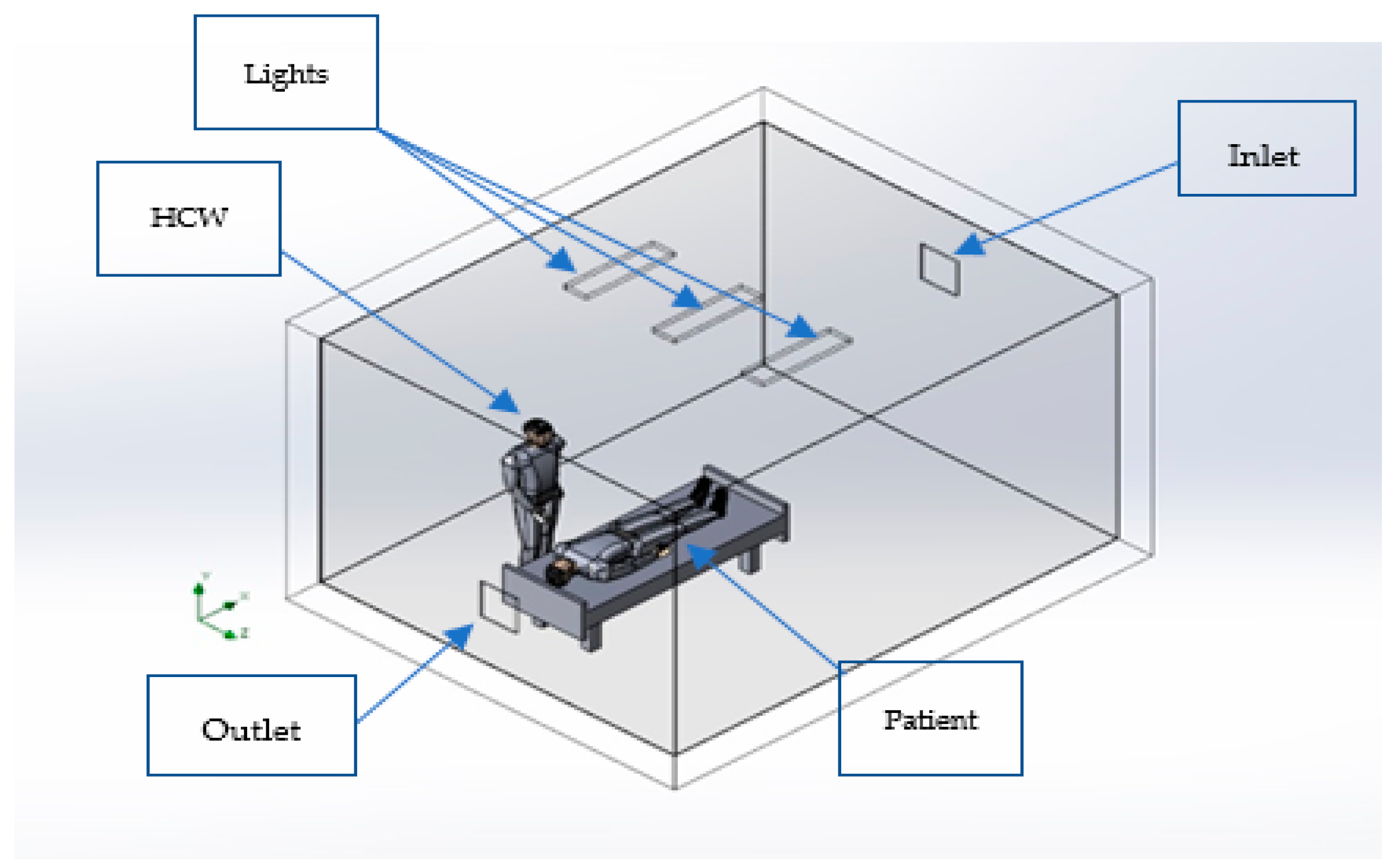
2.2. Model Description

A sample of a hospital isolation room (Table 1 and Table 2) was developed to conduct the present research. Inside the room, three models have been added. The first is the bed, then the health care worker (HCW) standing beside the bed and the patient lying on the bed. The air enters the room conditioned and refreshed at the inlet, while the contaminated air is eliminated through the outlet. Three light bulbs are mounted overhead, as shown in Figure 1. Previous studies suggested some designs that achieved optimum performance for either removing contaminants or enhancing thermal comfort. Based on that, we investigated how these designs influence the environment inside the space. As a result, the designs of (Figure 2a,b) were recommended by Çuhadaroğlu and Sungurlu [27], and the design of (Figure 2c) was selected by Thatiparti et al. [28]. Lastly, the design shown in (Figure 2d) was chosen by Cho [11] for optimal results.

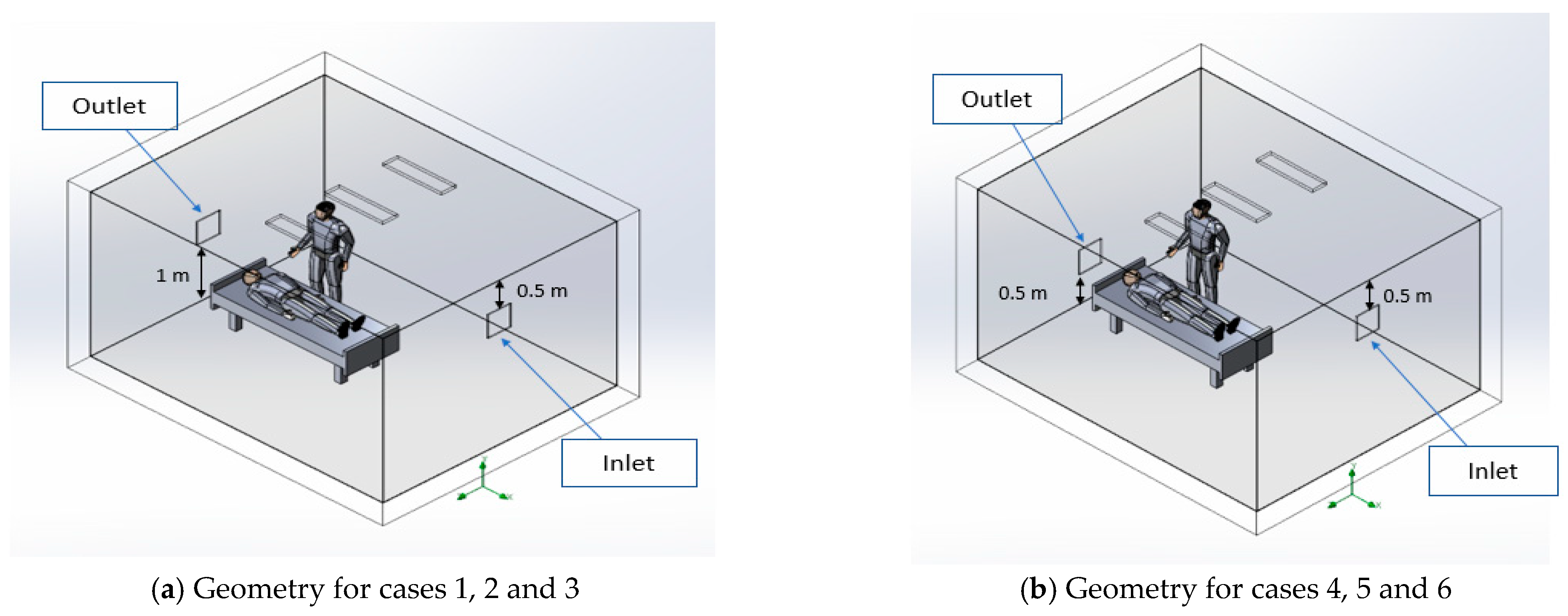
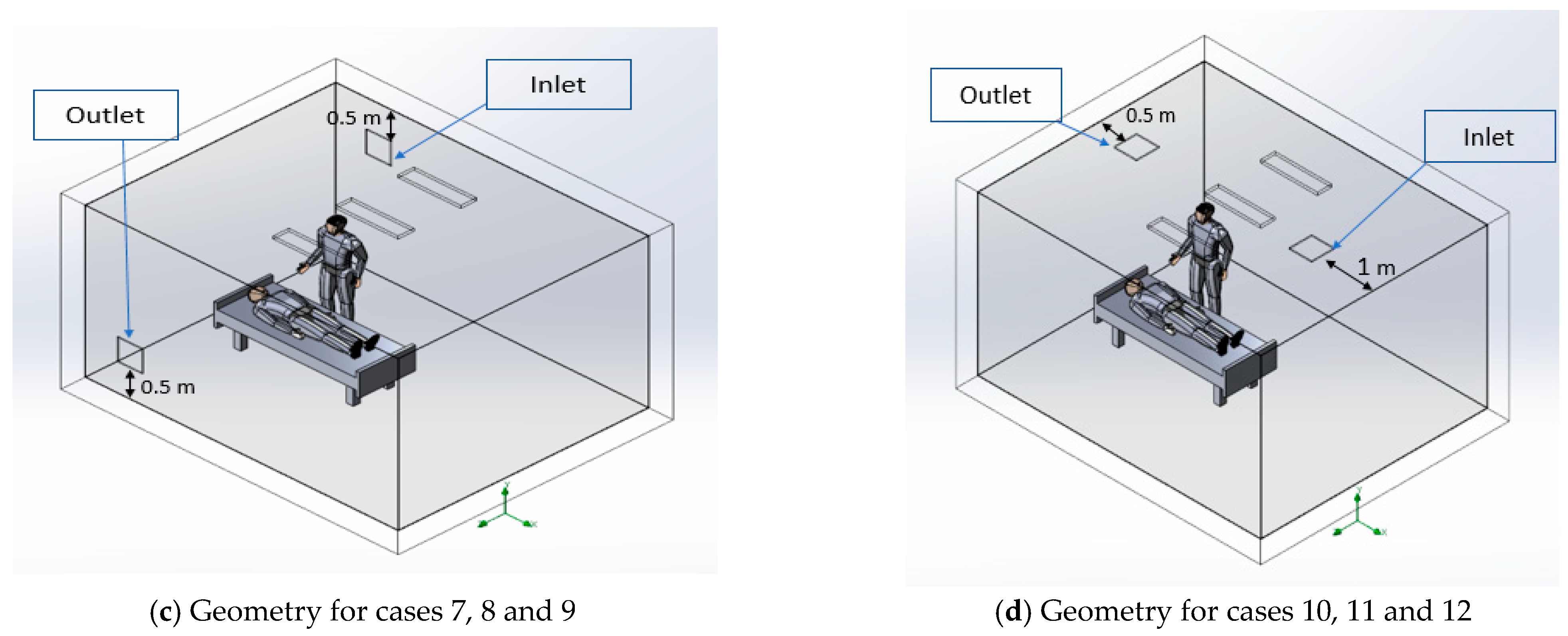
2.3. Boundary Conditions

Steady-state simulations are performed to verify pollutant concentration and thermal comfort through different ventilation designs. Initially, the airflow supply was maintained at 9   ACH with no return air [19]. Afterward, the 12   and   15   ACH were applied. For the system airborne infectious isolation rooms (AIIR), according to the American standard ASHRAE 170 [31], the pressure difference is essential to be maintained, and it was set at   2.5   Pa at the outlet. Heat sources for both the health care worker and patient, as well as the ceiling light, have been chosen to be 144   W / m 2 , 81   W / m 2 , and 11   W / m 2 , respectively [21,31]. In addition, it was assumed that the walls are adiabatic, with no heat transfer or storage within, and the air inlet temperature is 25   ° C , while the initial room temperature is 16   ° C , the pressure is 101,325   Pa and the relative humidity is 50 % . Moreover, pollutants are represented by carbon dioxide, which is excreted through the patient’s mouth with a mass flow of 0.00014   kg / s , at a temperature of 34   with 100 % humidity [19,32]. The turbulence intensity in the inlet was set at 20% within the recommended limits (10–30%) [33]. For the low-velocity value, 2% has been chosen in the range of 1–5% [34]. The length scale variation does not influence the flow pattern at a low inlet turbulence intensity value. However, its effect starts to appear from the 40% value of turbulence intensity. The turbulence length was chosen for both the inlet and the patient’s mouth based on the recommendations in reference [35].

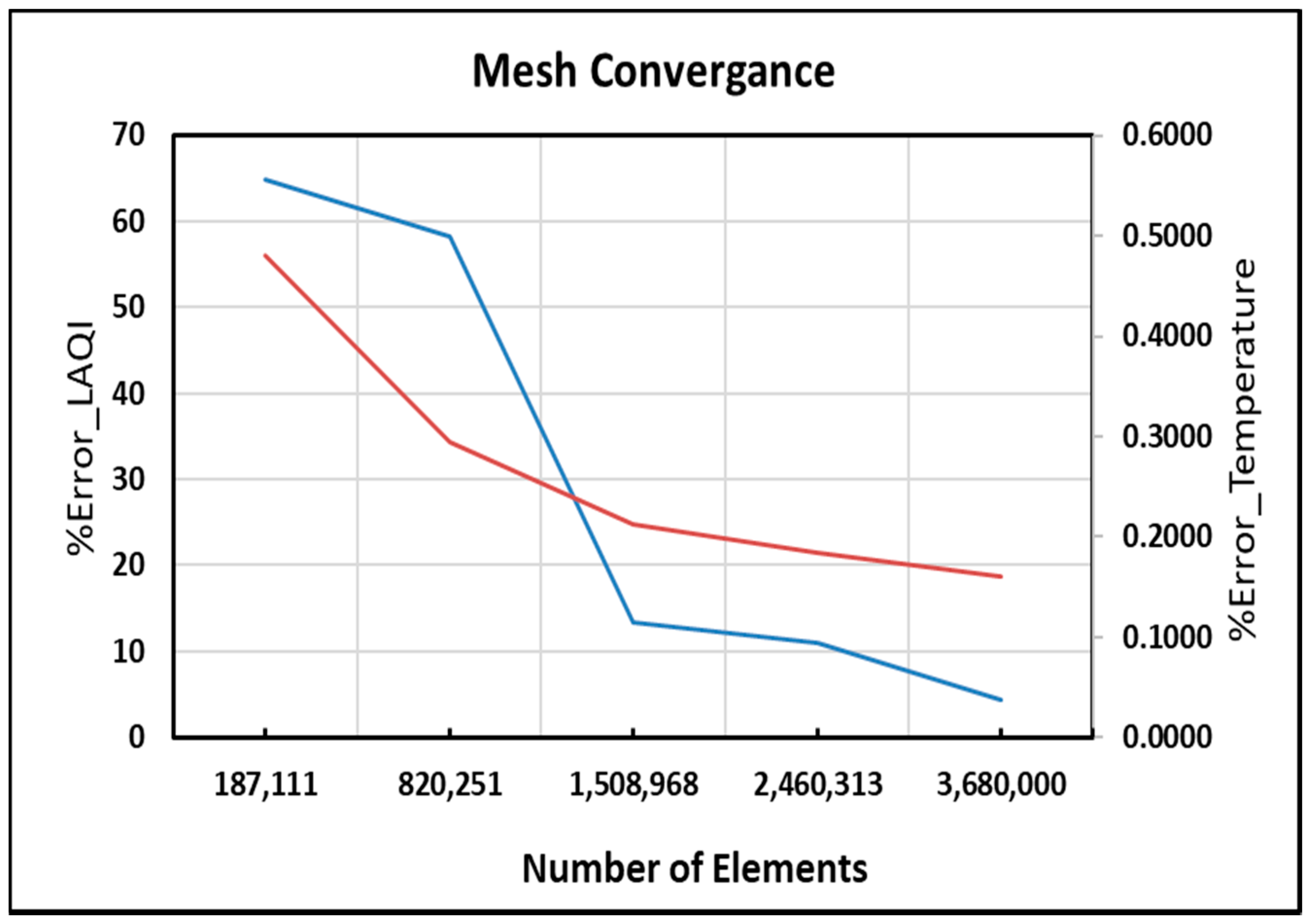
2.4. Mesh Independency Study and Solution Convergence Criteria

The domain has been split through a computational mesh along the coordinate system’s axes as rectangular parallelepipeds cells using a set of orthogonal planes. First, the original parallelepiped cells containing boundaries are split into several parts. The basic mesh is coarse. It is constructed for the whole domain at the beginning of the process and formed by dividing the domain by parallel planes into slices orthogonal to the Global Coordinate System’s axes. Next, the mesh is refined locally by splitting a cell into eight through three orthogonal planes that divide the cell’s edges into halves. The level of the initial mesh (Lini) is specified between (3–7) for each mesh, respectively, and the minimum gap size (hgap) is 0.01   m . This ensures that the flow passage through the gap is a width larger than the specified minimum gap size.
The local mesh was applied as a cube surrounding the occupants (the area of interest). The mesh is refined near the fluid/solid boundary to have the first grid point inside the viscous sublayer (y+ ≤ 5). We encountered convergence issues for higher values of y+ for the first grid point, although the study is steady state. Therefore, the log-law for the mean velocity near the walls is applied when 5 < y+ < 11.225, and the laminar stress–strain relationship is applied for lower values.
Furthermore, the enhanced wall treatment is applied for the standard k-epsilon with the low Reynolds model. This near-wall modeling method combines the two-layer model with enhanced wall functions [2,12,36]. Different grid sizes have been tested for accuracy. Five simulations were carried out from 125,843 to 3,680,531 cells to increase the precision of the results. An internal point was chosen in the domain to determine the temperature error throughout the refined meshes to assess mesh convergence. Figure 3 illustrates LAQI error fluctuation at the outlet for different mesh sizes. The convergence is achieved with a 2 million cells mesh.
Regarding the last two meshes (until 3.68 million cells), the convergence error is reduced to 4.43% for LAQI and less than 0.2% for the temperature, as shown in Figure 3. According to [2], a convergence error of less than 5% for the LAQI is acceptable. This accuracy is sufficient for doing the simulations, considering the power of the CPU, the domain magnitude, and the complicated curvy surfaces [37].
Convergence occurs when the solution no longer changes with successive iterations [24,25]. The convergence takes around 1100 iterations with a computation time of around 28 hours for each case on a single-processor desktop computer.

3. Results and Discussion

The results allow an understanding of how the mechanism of pollution transmission would be affected by adjusting the flow and the location of the air diffusers to find the optimum case through the results.

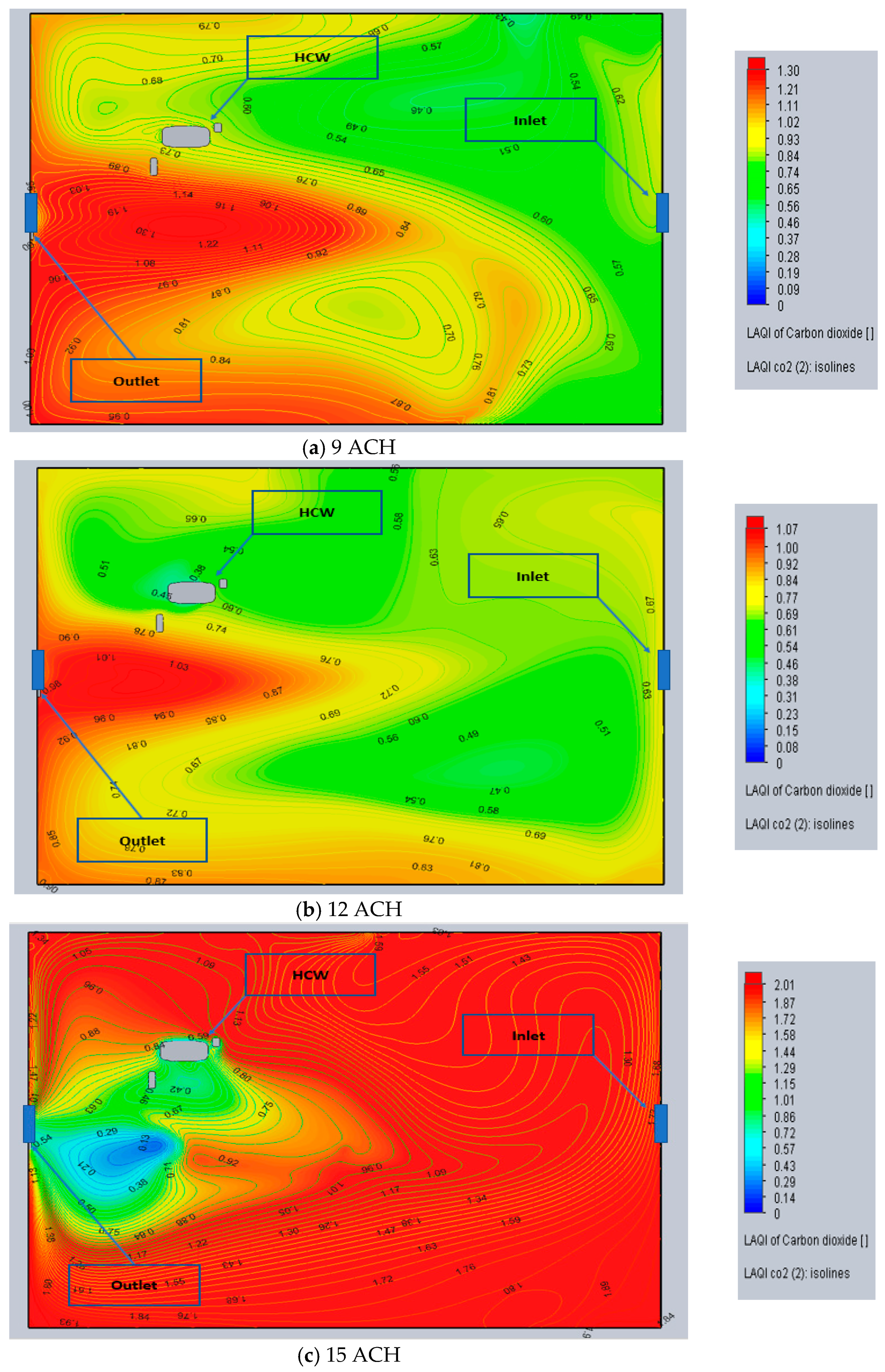
3.1. Cases 1, 2 and 3

As mentioned, each design has been tested using three cases with different airflows. In this design, the inlet is close to the ceiling at 0.5 m, and the outlet is located on the other side behind the patient at level 1 m from the floor, as shown in Figure 2a.

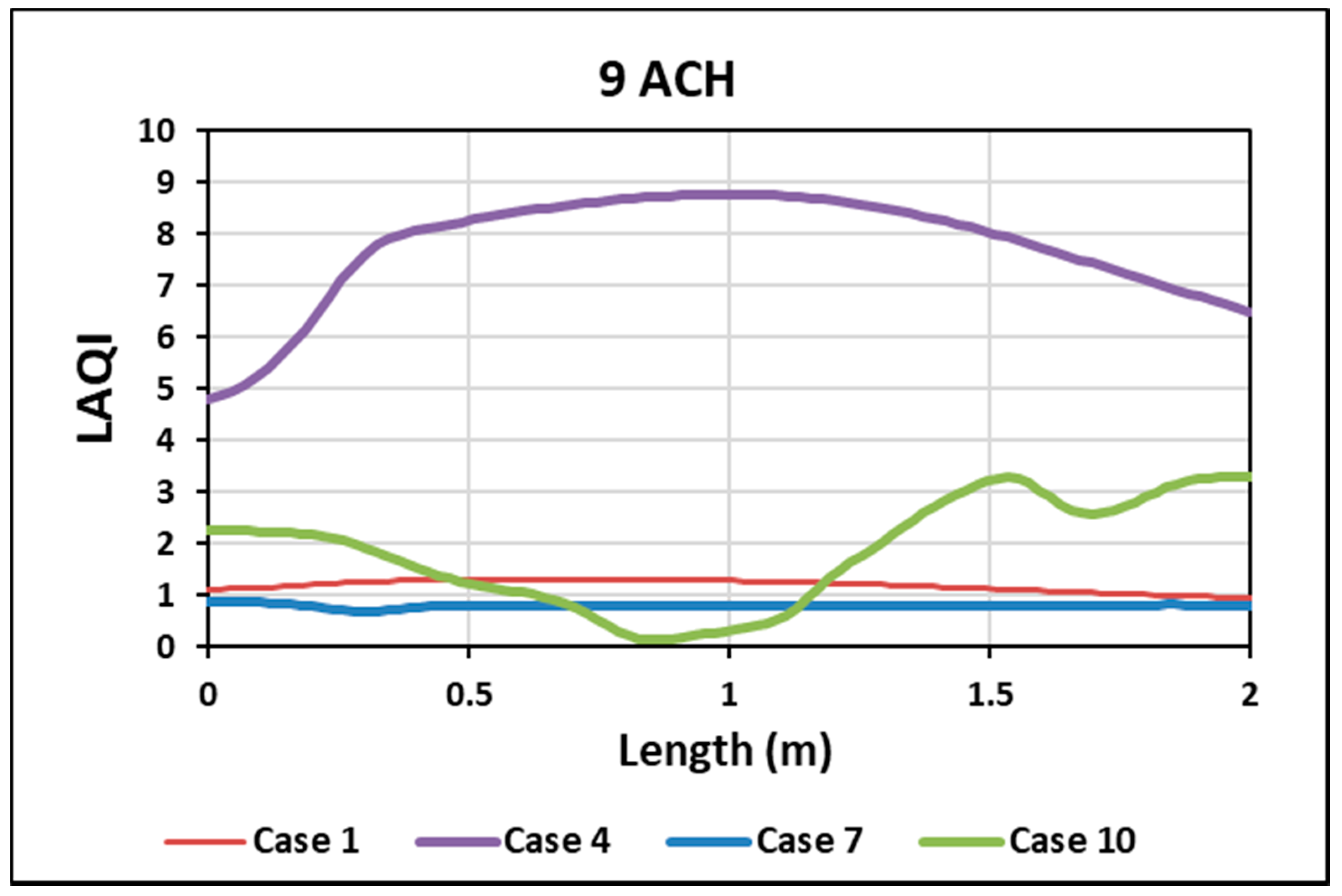
3.1.1. Local Air Quality Index (LAQI)

Using carbon dioxide as a proxy for the exhaled contaminant is one of the ways to study the air quality. Results were taken at the height of 1 m from the ground. Pollutant concentrations are lower when the value of LAQI is high. Figure 4a at 9 ACH indicates that the area near the exhaust is where most pollutants are removed, especially at the center of the outlet. LAQI gradually decreases away from the outlet.
In contrast, the HCW area behind the bed and the area near the inlet is characterized by a LAQI of approximately 0.6. It is less effective in removing contaminants as the force of the air is not strong enough to push the pollutants toward the outlet. This influence of ACH number on the airflow and the mixing process has also been illustrated by Berlanga, F. A. et al. [30].
At 12 ACH (Figure 4b), it can be observed that the removal is less effective at the lower part of the outlet level, while it is higher in the upper part, up to the inlet level. The removal effectiveness in the upper part will also be apparent in the the Trace Study of CO2 (Flow Trajectories) section of each case.

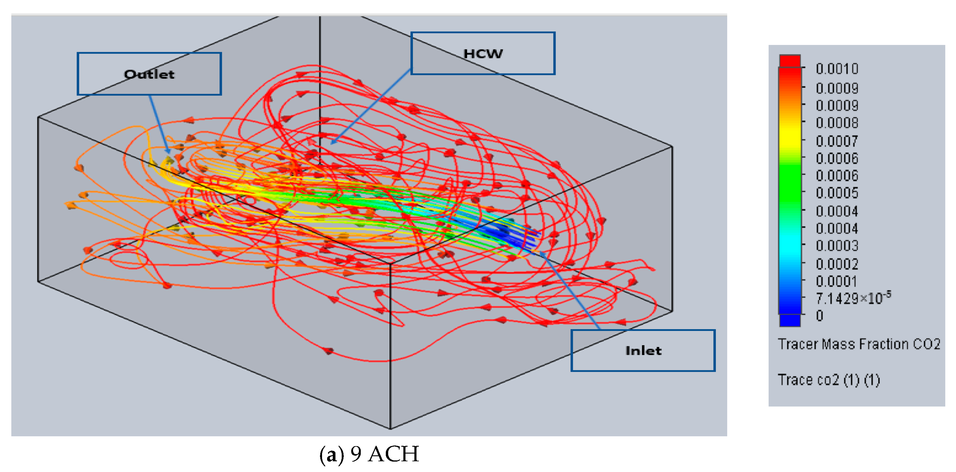
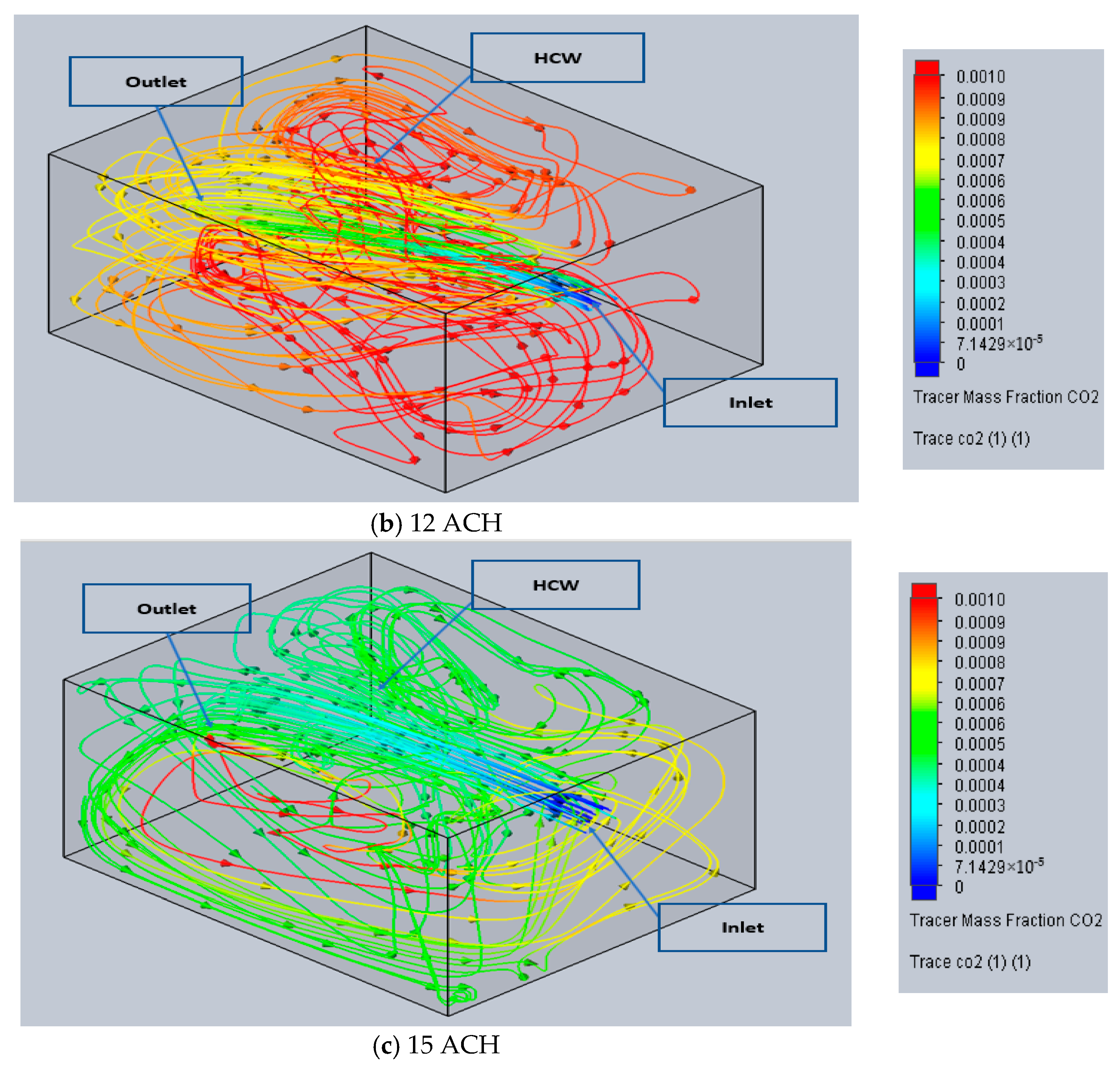
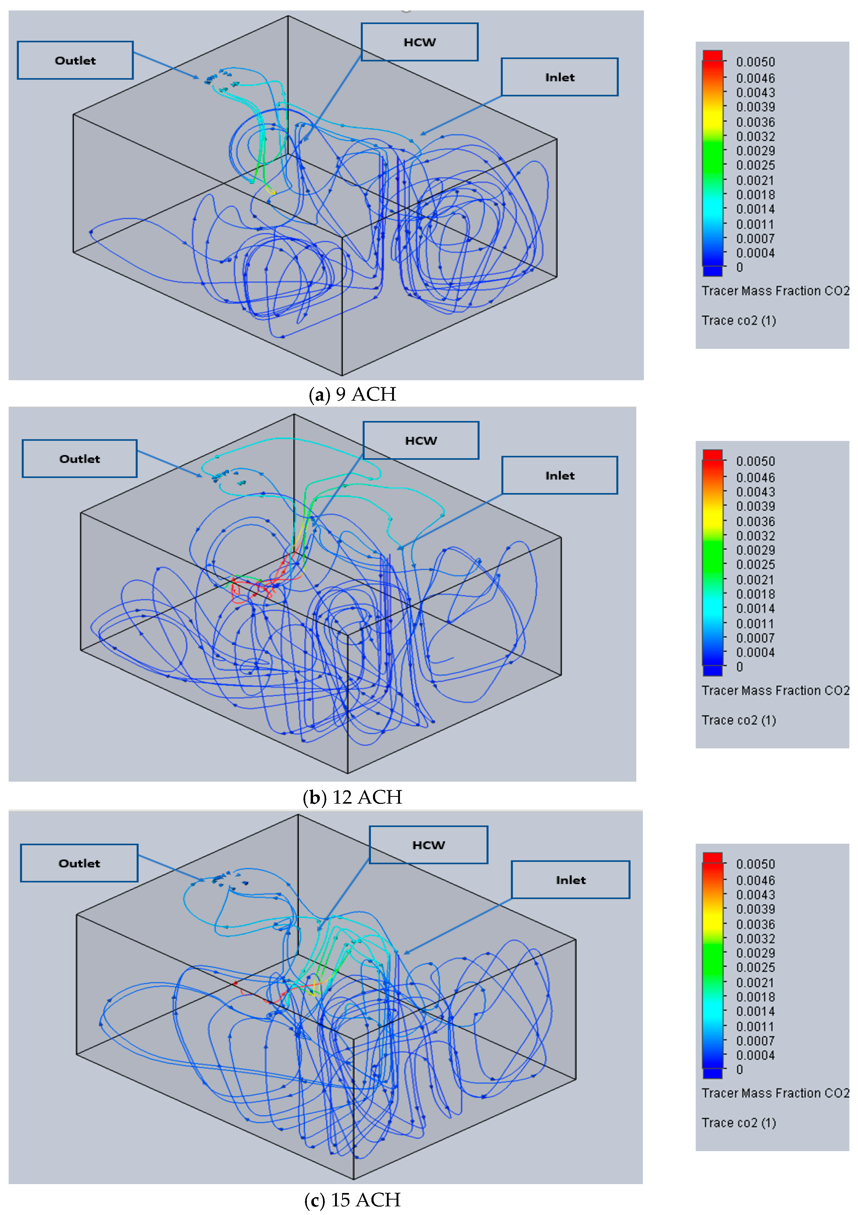
3.1.2. Tracer Study of CO2 (Flow Trajectories) Section of Each Case

When the ventilation increases to 15 ACH (Figure 4c), the pollutants are concentrated near the outlet. LAQI value is about 0.15 near the source (patient’s mouth), and 0.54 near the outlet as the particles are forced out of the outlet more quickly. However, the contaminants are extended over a larger area. This result agrees with Ameer et al. [26]. They found that a higher airflow velocity results in a larger polluted region with a lower concentration of pollutants, as the particles are forced out of the outlet more quickly. This finding corresponds with an experimental study concluding that an increased airflow decreases exposure to contaminants [30].

3.1.3. Tracer Study of CO2 (Flow Trajectories)

As mentioned, the pollutant is represented by the carbon dioxide emitted by the patient’s exhale, and its movement and concentration are explored over the room. The concentration is given as parts per million, ppm. The flow from the patient’s mouth has been considered 0.00014 kg/s. At a level of 1 m, there is noticeably less concentration at the outlet, around 0.0008 ppm, and about 0.001 ppm inside the air stream at 9 ACH (Figure 5a). However, at 12 ACH (Figure 5b), it is found that the mixing is more significant, and the pollutant concentration is approximately 0.00065 ppm lower on the opposite side of HCW. However, the area of HCW still has a high pollution concentration of about 0.0008 ppm. On the contrary, at 15 ACH (Figure 5c) demonstrates that a more extensive air volume circulation improves pollutant removal. The concentration is about 0.0004 ppm. These results correspond to a similar experimental study, which shows that a higher ACH increases removal [30] while some contaminants are still contained under the inlet at 0.0007 ppm.

3.2. Cases 4, 5 and 6

In the following cases, the design is similar to the previous one, with a different outlet location. The new position is 0.5 m from the floor instead of 1 m, as shown in Figure 2b.

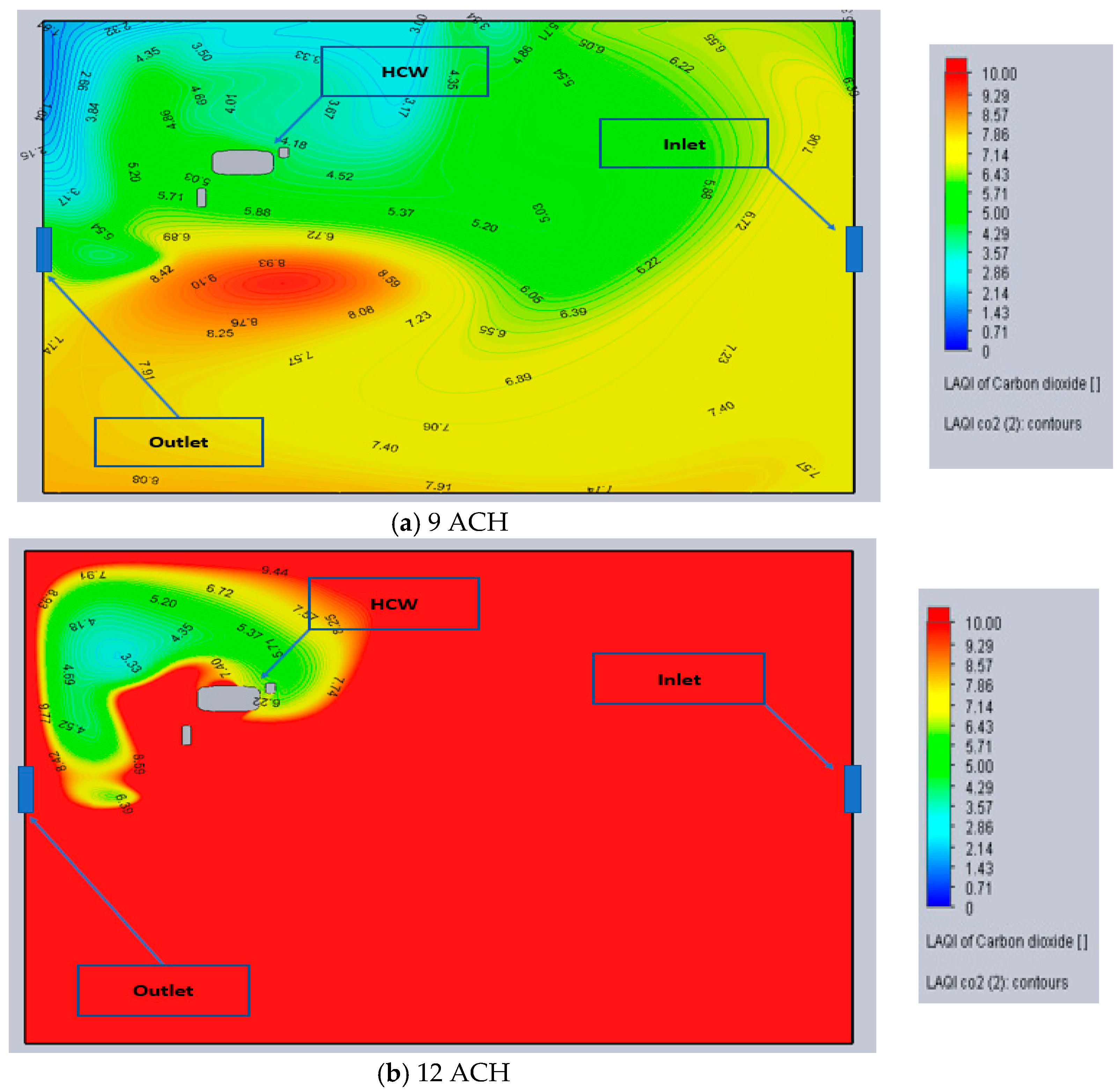
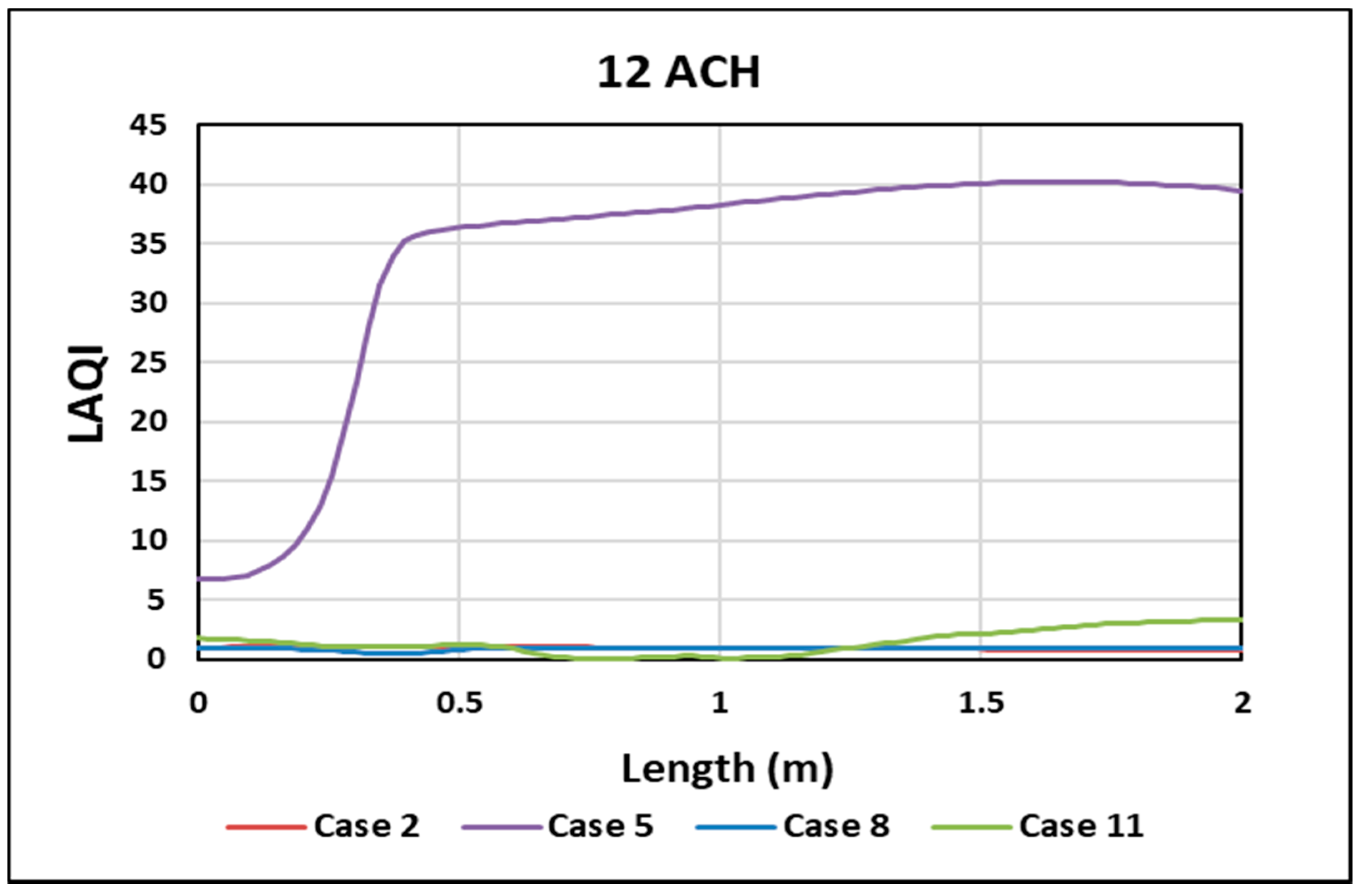
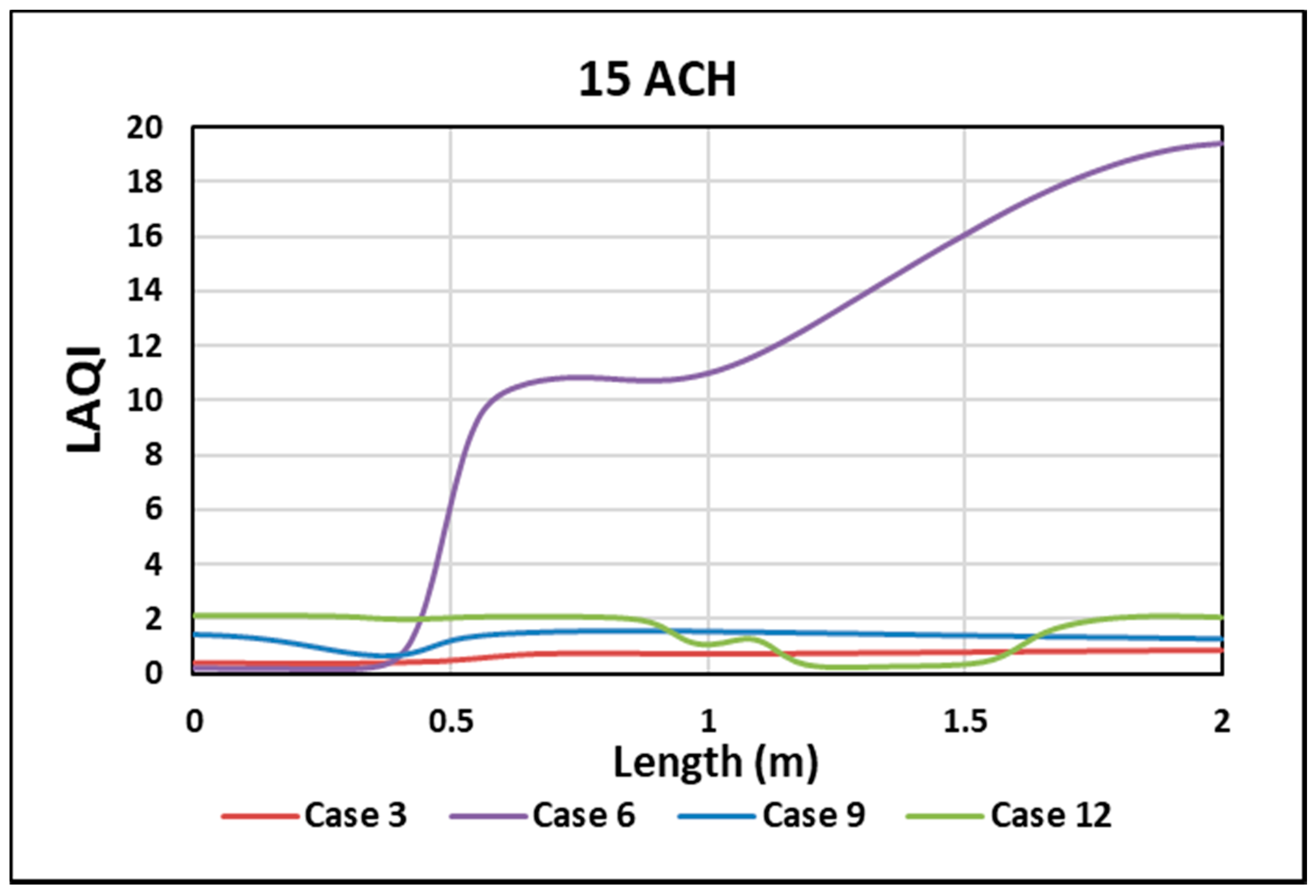
3.2.1. Local Air Quality Index (LAQI)

The elimination of pollutants after adjusting the outlet place at the level of the head is seen as supplementary and practical. This is due to removing pollutants from the patient’s mouth directly towards the outlet. This behavior corresponds to an experimental study showing that the outlet position affects the removal effectiveness [30].
The LAQI value in Figure 6a, at 9 ACH, is around 5 in the HCW area, while it is 0 in the area behind HCW, close to the corner. This area has a lot of contaminants due to the shortness of mixing.
In Figure 6b, for 12 ACH, the LAQI values are, in general, close to 10, which is excellent. However, the HCW area is still exposed to contamination, with LAQI values between 3.5–7.
For 15 ACH, in Figure 6c, the strong airflow and strategic placement of the outlet, as indicated by Ameer et al. [26], keep the whole room relatively clean. The most contaminated area is near the outlet and has a LAQI value of between 1.45 and 3.3.

3.2.2. Tracer Study of CO2 (Flow Trajectories)

Pollutant removal must also consider the pollutant’s particle circulation inside the room. The simulation results were shown for 9 ACH in (Figure 7a)). The presence of contaminants is at 0.0005 ppm behind the HCW, which is considered a high value. The majority of the area of the HCW side has contaminants around 0.0004 ppm. In Figure 7b, for 12 ACH, the concentration decreases in the same area to 0.0003 ppm.
On the other hand, near the outlet, the value exceeds 0.001 ppm due to the outlet being near the source of CO2 (patient’s mouth). Moreover, as shown in Figure 7c, for 15 ACH, almost all concentrations within the room are less than 0.0001 ppm except for the area above the bed. This configuration, associated with the ACH value and the outlet position, has been predicted and recommended by Berlanga, F. A. et al. [30].

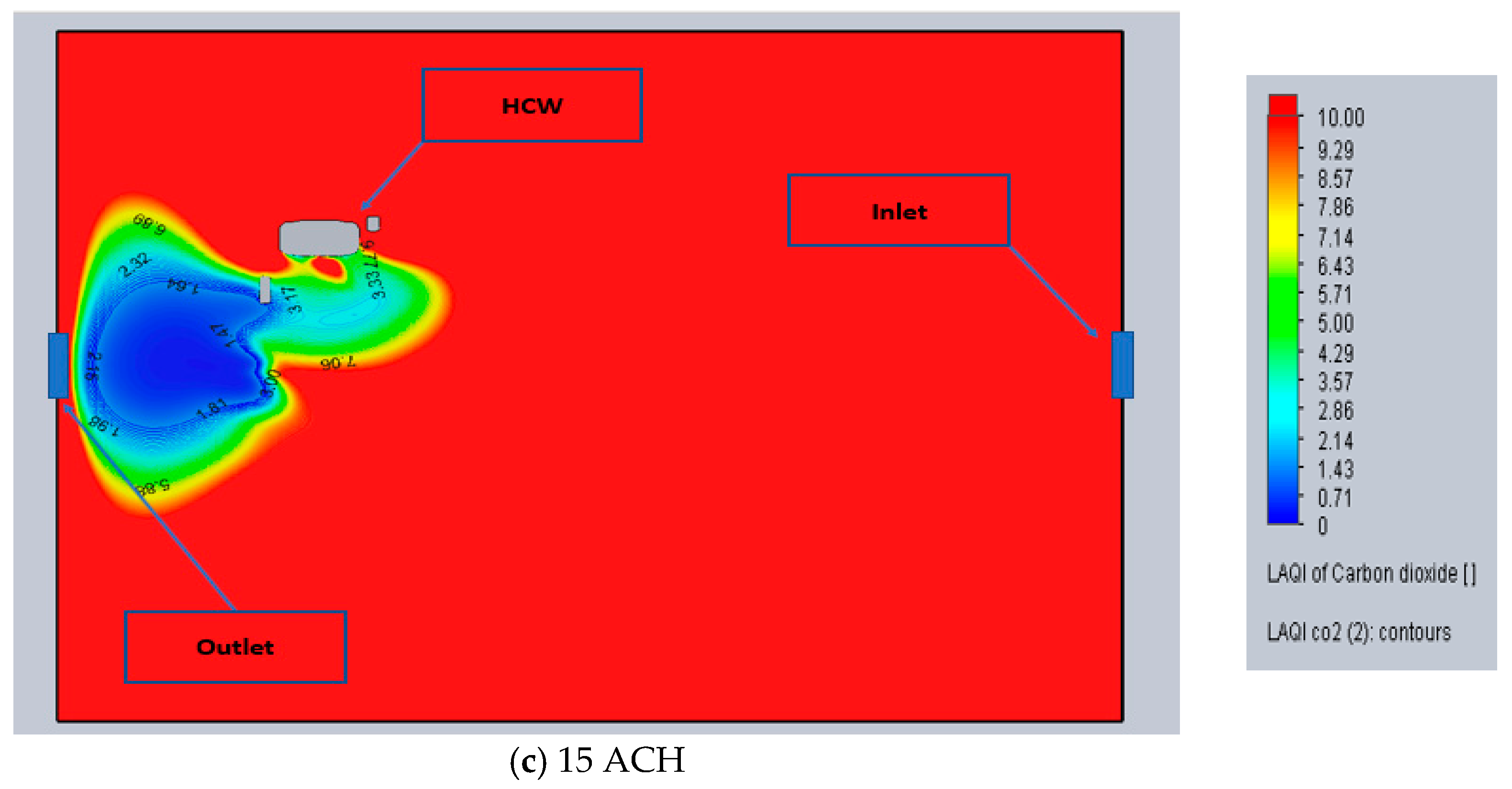
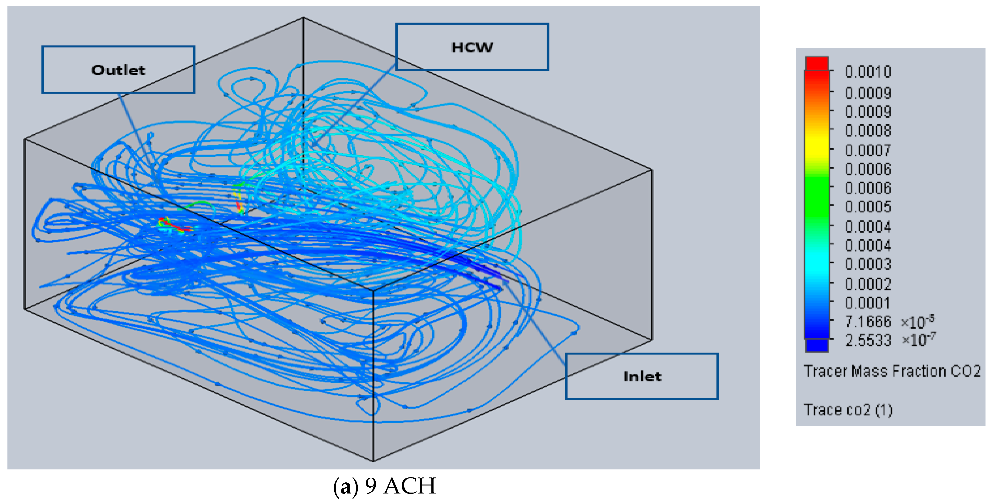
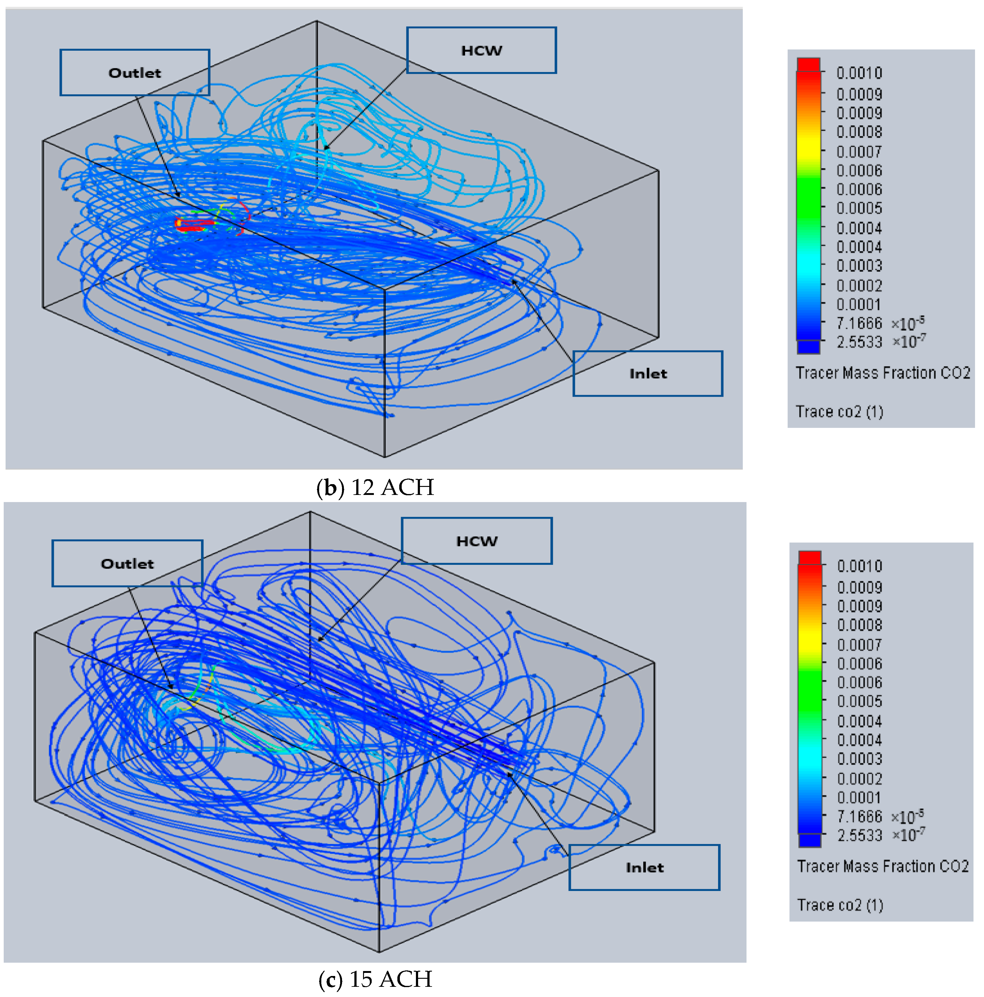
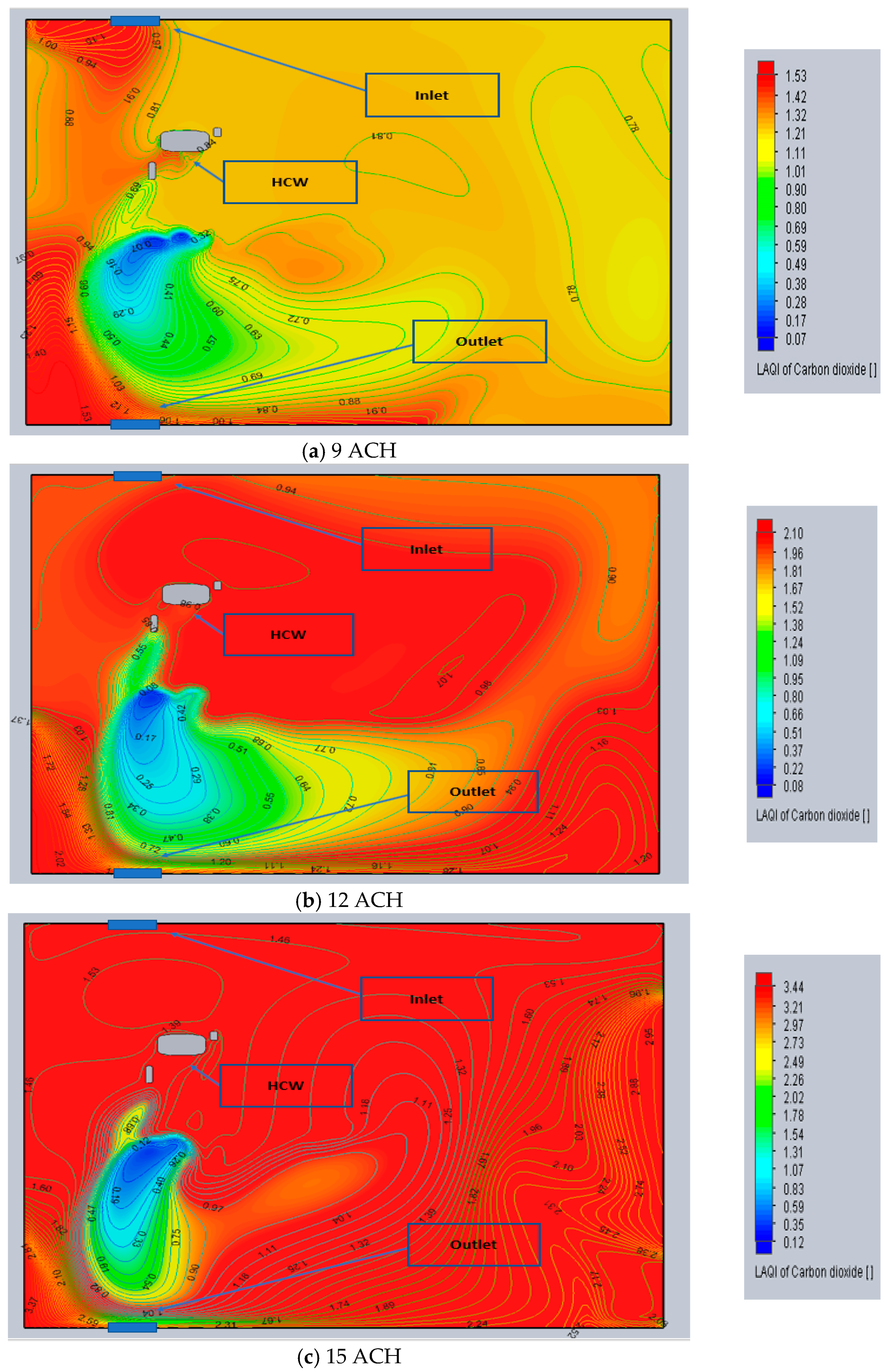
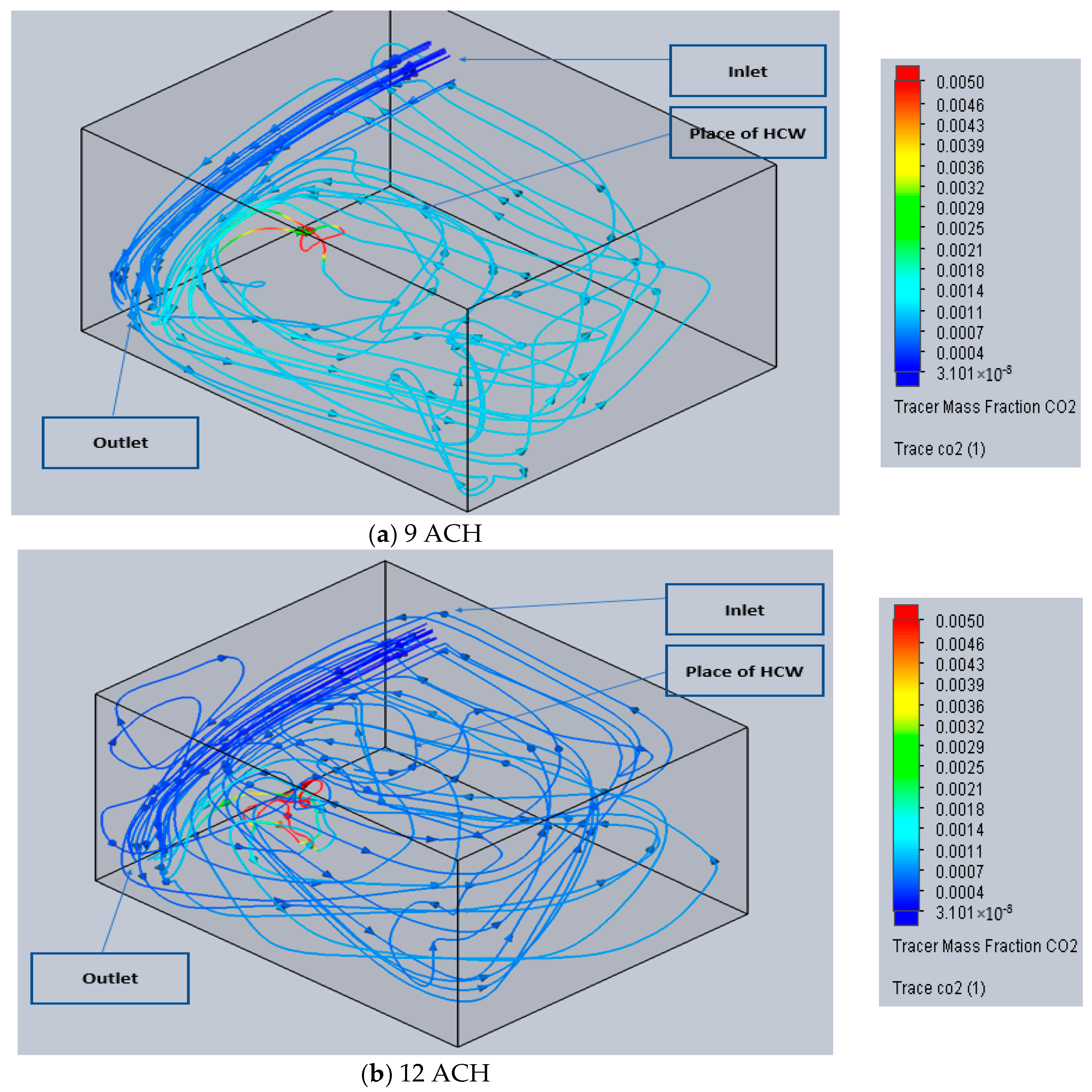
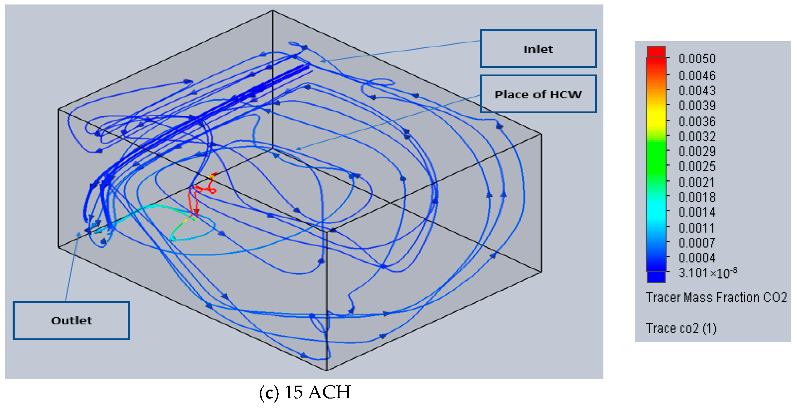
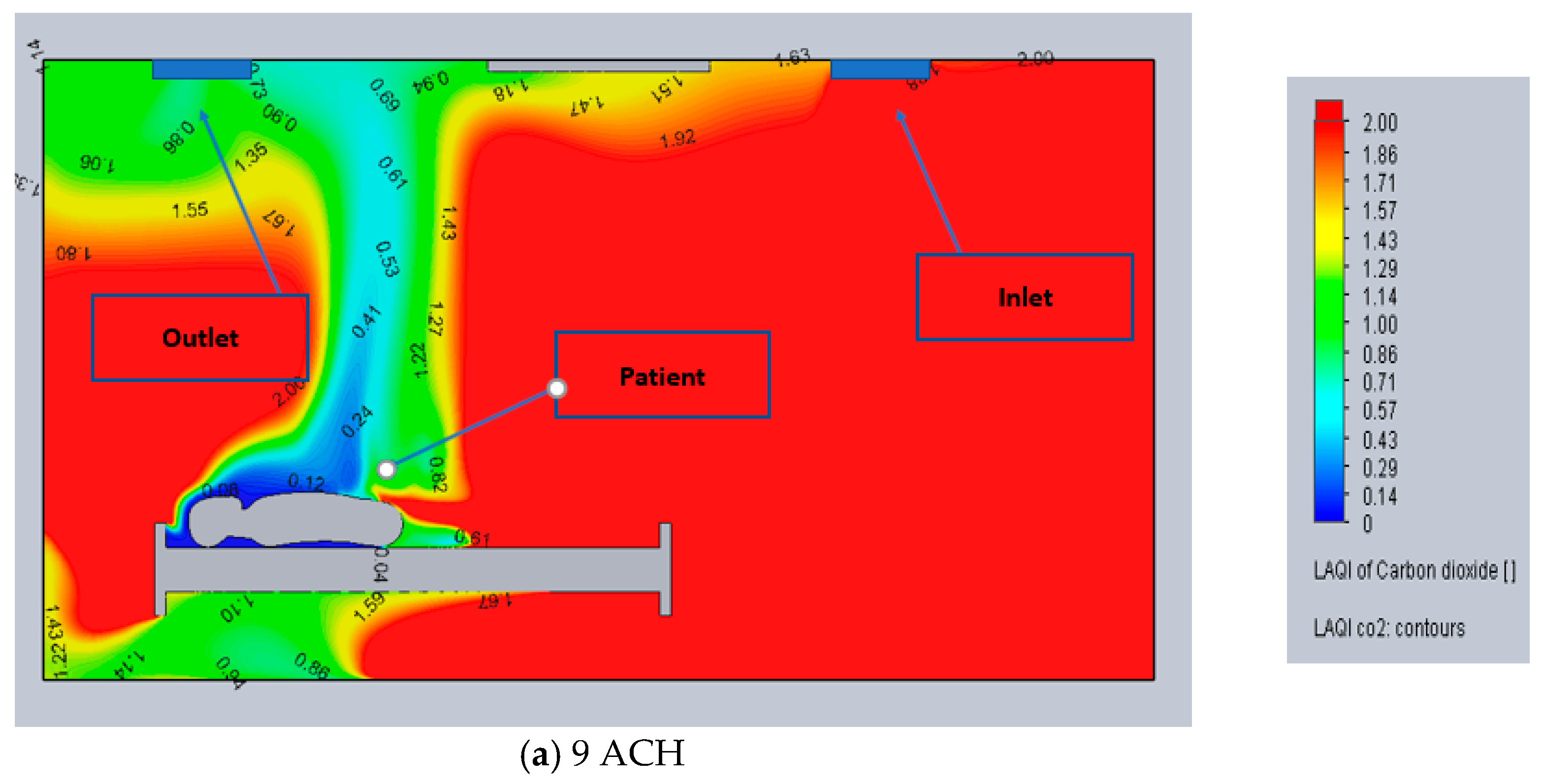
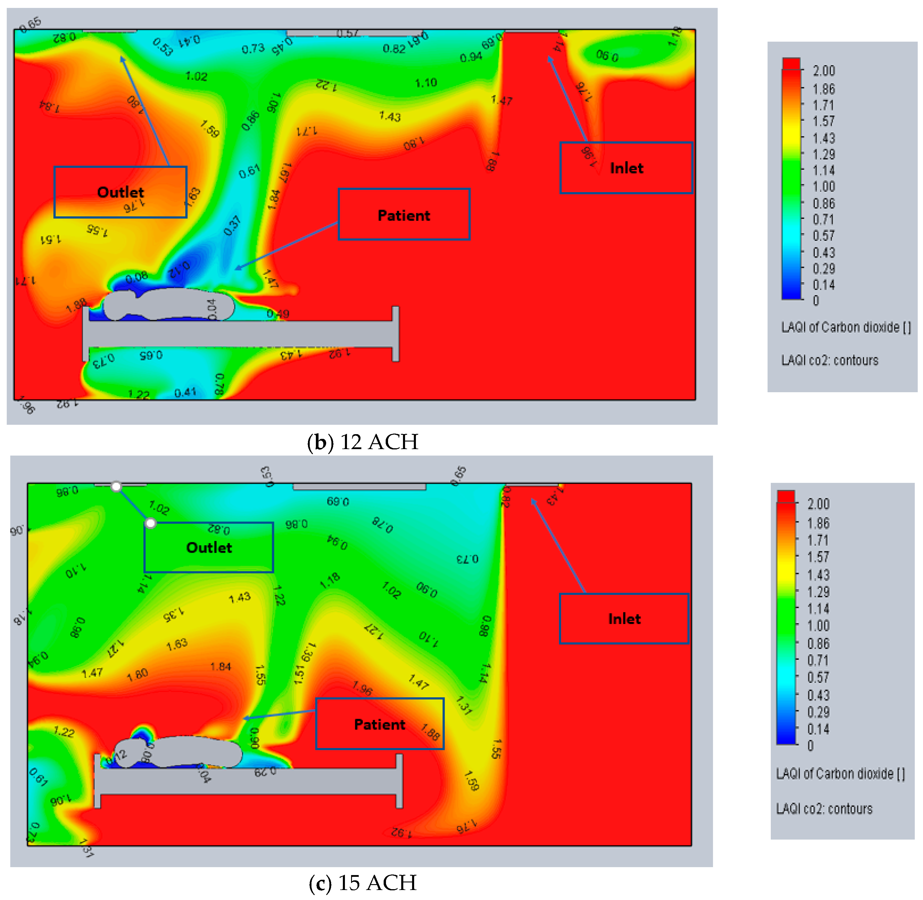
3.3. Cases 7, 8 and 9

In this design, the inlet is at the top of the wall behind the HCW at a distance of 0.5 m from the roof, and the outlet is located on the bottom, close to the floor on the other wall’s side at a distance of 0.5 m as shown in Figure 2c.

3.3.1. Local Air Quality Index (LAQI)

The placement of the inlet and outlet is a significant factor in determining how well pollutants are eliminated [26]. Figure 8a for 9 ACH shows that the area of minimum contamination appears on the right side of the HCW with LAQI values between 0.8 and 1. However, the region, as a whole, is still exposed to pollution due to the air pushing pollutants and not pulling them directly.
An improved contamination removal is observed at 12 ACH (Figure 8b), the area surrounding the HCW has a LAQI value near 0.95. However, there is still some spread toward the unoccupied region because of the air path, which makes the other side (close to the outlet) full of pollutants. It seems that the air velocity was not sufficient to remove the pollutants effectively.
The 15 ACH (Figure 8c) appears as the best flow rate for this design in eliminating pollutants based solely on the force of the air. As a result, most of the space has an optimum value of LAQI of more than 1, except the region between the pollutants source and the outlet. This result corresponds with the experimental study by Berlanga, F. A. et al. Furthermore, higher airflow enhances the elimination of the existing contaminants inside the space [30].

3.3.2. Tracer Study of CO2 (Flow Trajectories)

Figure 9a at 9 ACH shows that the pollutant concentration is reduced in the air path between the inlet and the outlet, which helps to ensure a clean area. The concentration near the patient is 0.0005 ppm. Nevertheless, the rest of the room has a concentration of approximately 0.0018 ppm, which corresponds with the outcomes from the LAQI analysis. For 12 ACH (Figure 9b), the results show the area far from the ventilation pathway has a slightly lower concentration, about 0.0011 ppm. As for 15 ACH (Figure 9c), the efficiency improves, where the values are approximately 0.0007 ppm for the unoccupied region. Kong X. et al. observed a similar impact of various ventilation systems on pollutant emissions through an experimental study [38].

3.4. Cases 10, 11 and 12

Both inlet and outlet are roof-mounted in this design. The distance from the side wall is 1 m for the inlet and 0.5 m for the outlet, as shown in Figure 2d.

3.4.1. Local Air Quality Index (LAQI)

As illustrated in Figure 10a for 9 ACH, the outlet absorbs contaminants emitted from the patient’s mouth, but some fall due to gravity and are stuck in the lower level. The value of LAQI starts around 0.1 close to the source, and it goes up gradually as the concentration of the contaminants reduces towards the outlet. At the same time, Figure 10b at 12 ACH results show that the increase in the airflow leads to more polluted regions. The mixing increases due to the higher airflow as emitting the pollutants here depends on the buoyancy. Low LAQI values are observed near the patient. At 15 ACH (Figure 10c), the contaminated area is confined near the inlet region towards the working area. Therefore, a correlation between airflow and pollution levels is noticed.

3.4.2. Tracer Study of CO2 (Flow Trajectories)

At 9 ACH, it can be seen in Figure 11a that the pollutants are present at a high concentration of about 0.004 PPM at the source location (patient’s mouth). It gradually decreases towards the outlet, while the unoccupied area has a minor concentration of around 0.0004 ppm. As shown in Figure 11b at 12 ACH, the mixing of pollutants increases, which helps spread their concentration over a larger volume, especially the HCW side, where the result is 0.0035 ppm. The airflow increase affects the distribution of these pollutants around the space. At 15 ACH, as seen in (Figure 11c), there is a similar effect with case 11 at 12 ACH, the region where the inlet exists has lower contaminants, with a value of 0.0004 ppm. Referring to the inlet location in this design, removing the contaminants is considered inappropriate. This confirms the results of the experimental study [30], which found that the ventilation performance of the side inlet/ outlet design was significantly higher than that of the top inlet/outlet design.

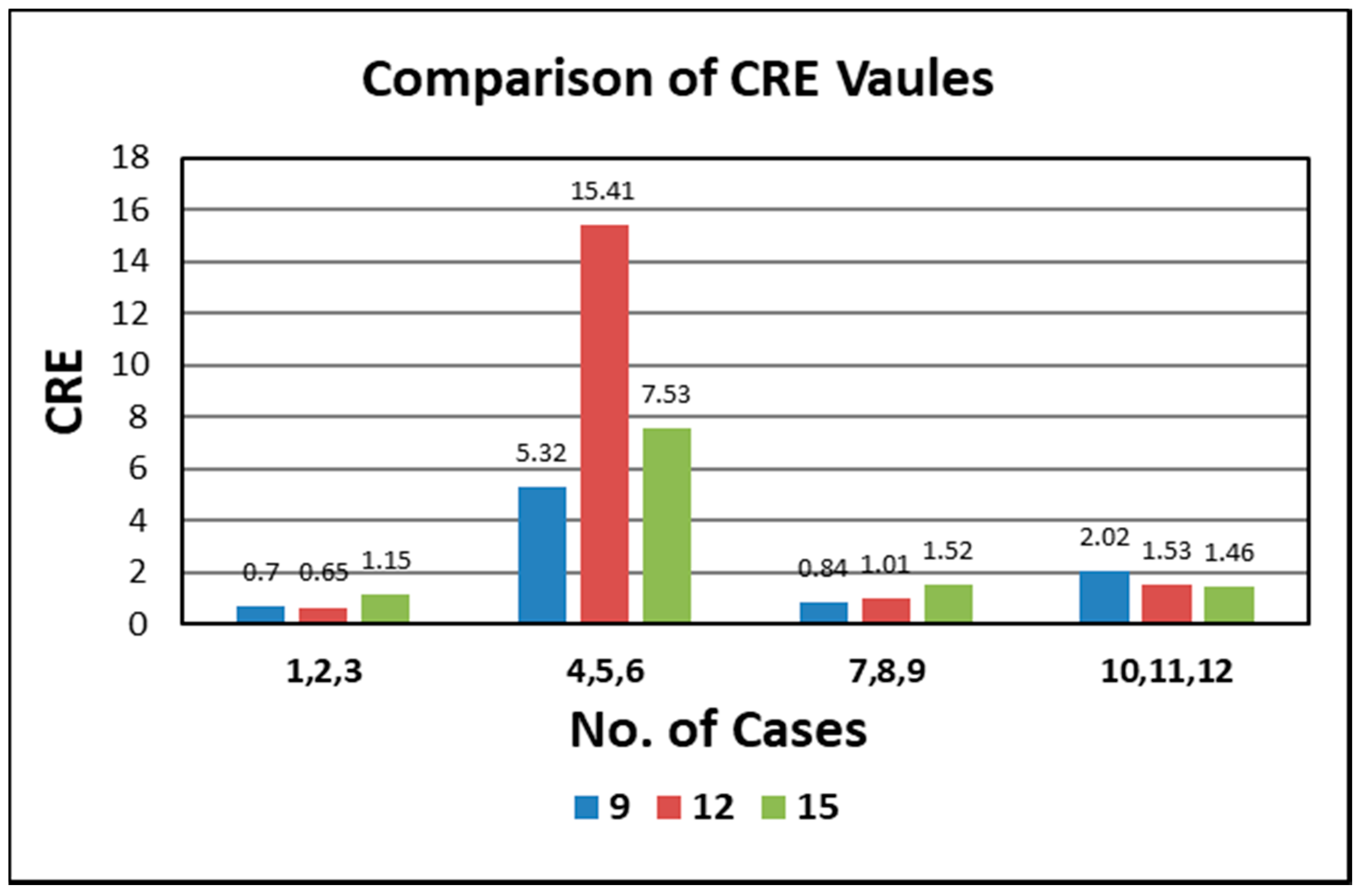
3.5. Contaminant Removal Effectiveness (CRE)

In the diagram in Figure 12, it can be noticed from the model (Figure 2b) that the best CRE values occur in cases 4, 5, and 6, where the outlet is situated close to the head at a low elevation. Compared to other designs, this one effectively removed contaminants from the space. At the same time, a similar design (Figure 2a) was used for cases 1, 2, and 3, where the outlet was situated above the patient’s head, resulting in an undesirable outcome. Meanwhile, for the third design, case 9 at 15 ACH (Figure 2c) has the optimum CRE with a value of more than 1.5. Finally, in the fourth design case (10, 11, and 12) illustrated in Figure 2d, all of these airflows achieved the minimum required contaminant removal performance.
The following charts are drawn along a 2 m horizontal line located 1 m from the ground, above and parallel to the patient. We compare LAQI through aeration value. Results in Figure 13 and Figure 14 illustrate the excellent values for pollutant removal efficiency in cases 4 and 5. However, case 6 at 15 ACH, as shown in Figure 15, does not show adequate results at the beginning of the bed area where the contaminants’ source exists. Away from the patient’s mouth, LAQI values rise dramatically. The other cases, even with the proximity from the outlet, still have low and fluctuating values, which could not be recommended.

4. Conclusions

Ventilation dramatically impacts human health because of its effect on the dispersal of contaminants like SRAS-COVID-19. Therefore, it is crucial to have a ventilation system that can prevent the spread and decrease the transmission of contaminants in buildings, especially in healthcare facilities. Cases 4, 5, and 6 of the second design yielded optimum results for pollution removal. All the cases achieved a CRE value higher than 5. The contaminants were removed quickly due to the proximity of the outlet to the source of CO2. The outlet is located at 0.5 m from the floor in these cases. These cases correspond to the conclusions of Cho [11].
On the other hand, the worst position for the outlet was in the first design, where the outlet was above the level of the patient in cases 1, 2, and 3. In this configuration, case 3 is the only one with a CRE value higher than 1. However, in cases 3 and 6, at 15 ACH, the airflow becomes horizontal due to the force of air which overcomes gravity.
The analysis shows that LAQI values are of similar magnitude, except for cases 4, 5, and 6, which show significantly better performances. These results correspond with several experimental studies, showing similar performances for different airflow intensities and inlet/outlet positions [30]. Additionally, dead zones should be avoided; the airflow cannot reach these regions to improve the removal of the contaminants [13].
Despite abundant studies in this field, considerable effort is still required to identify the best solutions. In addition, many difficulties remain during the modeling process, such as the magnitude of the model and the human body’s unique design, making meshing challenging. Furthermore, the experimental work will play a vital part in confirming the outcomes alongside these simulations.

Author Contributions

Conceptualization, M.A.; methodology, M.A.; software, M.A.; validation, M.A.; formal analysis, M.A.; investigation, M.A.; resources, M.A.; data curation, M.A.; writing—original draft preparation, M.A., A.I.; writing—review and editing, M.A., A.I. and M.Y.H.; visualization, M.A., A.I.; supervision, A.I. and M.Y.H.; project administration, A.I. and M.Y.H.; funding acquisition, A.I. All authors have read and agreed to the published version of the manuscript.

Funding

The authors acknowledge the financial contribution from the Natural Sciences and Engineering Research Council (NSERC) Canada through a Discovery Grant.

Data Availability Statement

Not applicable.

Conflicts of Interest

The authors declare no conflict of interest.

References

  1. Borro, L.; Mazzei, L.; Raponi, M.; Piscitelli, P.; Miani, A.; Secinaro, A. The role of air conditioning in the diffusion of Sars-CoV-2 in indoor environments: A first computational fluid dynamic model, based on investigations performed at the Vatican State Children’s hospital. Environ. Res. 2021, 193, 110343. [Google Scholar] [CrossRef] [PubMed]
  2. Hallé. Prediction of Bioparticles Dispersion and Distribution in a Hospital Isolation Room. Ph.D. Thesis, École De Technologie Supérieure, Montreal, QC, Canada, 2016. [Google Scholar]
  3. Anuraghava, C.; Abhiram, K.; Reddy, V.N.; Rajan, H. CFD modelling of airborne virus diffusion characteristics in a negative pressure room with mixed mode ventilation. Int. J. Simul. Multidiscip. Des. Optim. 2021, 12, 1. [Google Scholar] [CrossRef]
  4. Novoselac, A.; Srebric, J. Comparison of air exchange efficiency and contaminant removal effectiveness as IAQ indices. Trans.-Am. Soc. Heat. Refrig. Air Cond. Eng. 2003, 109, 339–349. Available online: https://www.caee.utexas.edu/prof/novoselac/Publications/Novoselac_ASHRAE_Transactions_2003.pdf (accessed on 11 July 2003).
  5. Tian, X.; Zhang, S.; Awbi, H.B.; Liao, C.; Cheng, Y.; Lin, Z. Multi-indicator evaluation on ventilation effectiveness of three ventilation methods: An experimental study. Build Environ. 2020, 1, 180. [Google Scholar] [CrossRef]
  6. Daisey, J.M.; Angell, W.J.; Apte, M.G. Indoor Air Quality, Ventilation And Health Symptoms In Schools: An Analysis Of Existing Information. Indoor Air Berkeley USA 2003, 13, LBNL-48287. [Google Scholar] [CrossRef] [Green Version]
  7. American Society of Heating R and ACEngineers. HVAC Design Manual for Hospitals and Clinics. 2012. 301p. Available online: https://www.ashrae.org/technical-resources/bookstore/hvac-design-manual-for-hospitals-and-clinics (accessed on 11 July 2003).
  8. Bolashikov, Z.D.; Melikov, A.K.; Kierat, W.; Popioek, Z.; Brand, M. Exposure of health care workers and occupants to coughed airborne pathogens in a double-bed hospital patient room with overhead mixing ventilation. HVAC R Res. 2012, 18, 602–615. [Google Scholar]
  9. Chow, T.T.; Kwan, A.; Lin, Z.; Bai, W. Conversion of operating theatre from positive to negative pressure environment. J. Hosp. Infect. 2006, 64, 371–378. [Google Scholar] [CrossRef]
  10. Alhamid, M.I.; Budihardjo Raymond, A. Design of the ventilation system and the simulation of air flow in the negative isolation room using FloVent 8.2. AIP Conf. Proc. 2018, 1984, 020016. [Google Scholar]
  11. Cho, J. Investigation on the contaminant distribution with improved ventilation system in hospital isolation rooms: Effect of supply and exhaust air diffuser configurations. Appl. Therm. Eng. 2019, 148, 208–218. [Google Scholar] [CrossRef]
  12. Mousavi. Airborne Infection in Healthcare Environments: Implications to Hospital Corridor Design [Internet]. 2015. Available online: http://digitalcommons.unl.edu/constructiondisshttp://digitalcommons.unl.edu/constructiondiss/21 (accessed on 17 July 2015).
  13. Abhinav, R.; Sunder, P.B.S.; Gowrishankar, A.; Vignesh, S.; Vivek, M.; Kishore, V.R. Numerical study on effect of vent locations on natural convection in an enclosure with an internal heat source. Int. Commun. Heat Mass Transf. 2013, 49, 69–77. [Google Scholar] [CrossRef]
  14. Abdel, K.; Saadeddin, R. The Effects of Diffuser Exit Velocity and Distance Between Supply The Effects of Diffuser Exit Velocity and Distance Between Supply and Return Apertures on the Efficiency of an Air Distribution and Return Apertures on the Efficiency of an Air Distribution System in an Office Space System in an Office Space [Internet]. 2016. Available online: https://openprairie.sdstate.edu/etd (accessed on 5 February 2016).
  15. Kokkonen, A.; Hyttinen, M.; Holopainen, R.; Salmi, K.; Pasanen, P. Performance testing of engineering controls of airborne infection isolation rooms by tracer gas techniques—Enhanced Reader. Indoor Built Environ. 2014, 23, 994–1001. [Google Scholar] [CrossRef]
  16. Villafruela, J.M.; Olmedo, I.; Berlanga, F.A.; Ruiz de Adana, M. Assessment of displacement ventilation systems in airborne infection risk in hospital rooms. PLoS ONE 2019, 1, 14. [Google Scholar] [CrossRef] [PubMed]
  17. Yam, R.; Yuen, P.L.; Yung, R.; Choy, T. Rethinking hospital general ward ventilation design using computational fluid dynamics. J. Hosp. Infect. 2011, 77, 31–36. [Google Scholar] [CrossRef] [PubMed]
  18. Mousavi, E.S.; Grosskopf, K.R. Ventilation Rates and Airflow Pathways in Patient Rooms: A Case Study of Bioaerosol Containment and Removal. Ann. Occup. Hyg. 2014, 59, 1190–1199. [Google Scholar] [CrossRef] [Green Version]
  19. Lu, Y.; Oladokun, M.; Lin, Z. Reducing the exposure risk in hospital wards by applying stratum ventilation system. Build Environ. 2020, 183, 107204. [Google Scholar] [CrossRef]
  20. Fan, M.; Fu, Z.; Wang, J.; Wang, Z.; Suo, H.; Kong, X.; Li, H. A review of different ventilation modes on thermal comfort, air quality and virus spread control. Build. Environ. 2022, 212, 108831. [Google Scholar] [CrossRef] [PubMed]
  21. Ahmed, T. Performance Investigation of Building Ventilation System by Calculating Comfort Criteria through HVAC Simulation. IOSR J. Mech. Civ. Eng. 2012, 3, 7–12. [Google Scholar] [CrossRef]
  22. Risberg, D. Daniel Risberg Analysis of the Thermal Indoor Climate with Computational Fluid Dynamics for Buildings in Sub-arctic Regions. Ph.D. Thesis, Luleå University of Technology, Luleå, Sweden, 2018. [Google Scholar]
  23. Ghanta, N. Meta-Modeling and Optimization of Computational Fluid Dynamics (CFD) Analysis in Thermal Comfort for Energy-Efficient Chilled Beams-Based Heating, Ventilation and Air-Conditioning (HVAC) Systems. Ph.D. Thesis, Massachusetts Institute of Technology, Cambridge, MA, USA, May 2020. [Google Scholar]
  24. Solidworks Flow Simulation. Technical Reference Solidworks Flow Simulation. 2021. Available online: https://www.solidworks.com/product/solidworks-flow-simulation (accessed on 5 February 2021).
  25. Mekbib Kifle, P. CFD Simulation of Heavily Insulated Office Cubicle Heated by Ventilation Air Done in Collaboration with [Internet]. 2018. Available online: https://www.oslomet.no (accessed on 23 May 2018).
  26. Azmi, M.A.; Hassan, N.N.; Salleh, Z.M. Investigation of Airflow in A Restaurant to Prevent COVID-19 Transmission Using CFD Software. Prog. Eng. Appl. Technol. 2021, 3, 977–991. [Google Scholar]
  27. Çuhadaroğlu, B.; Sungurlu, C. ID 8-A CFD analysis of air distributing performance of a New Type HVAC Diffuser. 2015. Available online: https://www.researchgate.net/publication/288324226_ID_8_-A_CFD_analysis_of_air_distributing_performance_of_a_New_Type_HVAC_Diffuser. (accessed on 27 December 2015).
  28. Thatiparti, D.S.; Ghia, U.; Mead, K.R. Computational fluid dynamics study on the influence of an alternate ventilation configuration on the possible flow path of infectious cough aerosols in a mock airborne infection isolation room. Sci. Technol. Built. Environ. 2017, 23, 355–366. [Google Scholar] [CrossRef] [Green Version]
  29. Solidworks Flow Simulation 201. 2021. Available online: https://www.solidworks.com/media/solidworks-2021-flow-simulation (accessed on 5 February 2021).
  30. Berlanga, F.A.; Olmedo, I.; de Adana, M.R.; Villafruela, J.M.; José, J.F.S.; Castro, F. Experimental assessment of different mixing air ventilation systems on ventilation performance and exposure to exhaled contaminants in hospital rooms. Energy Build. 2018, 177, 207–219. [Google Scholar] [CrossRef] [Green Version]
  31. Ventilation of Health Care Facilities [Internet]. 2020. Available online: https://www.ashrae.org (accessed on 5 February 2020).
  32. Yoon, S.H.; Ahn, H.S.; Choi, Y.H. Numerical Study To Evaluate The Characteristics Of Hvac-Related Parameters To Reduce CO2 Concentrations In Cars. Int. J. Automot. Technol. 2016, 17, 959–966. [Google Scholar] [CrossRef]
  33. Cehlin, M.; Moshfegh, B. Numerical modeling of a complex diffuser in a room with displacement ventilation. Build. Environ. 2010, 45, 2240–2252. [Google Scholar] [CrossRef]
  34. Cao, G.; Ruponen, M.; Paavilainen, R.; Kurnitski, J. Modelling and simulation of the near-wall velocity of a turbulent ceiling attached plane jet after its impingement with the corner. Build. Environ. 2011, 46, 489–500. [Google Scholar] [CrossRef]
  35. Gao, N.; Niu, J. Transient CFD simulation of the respiration process and inter-person exposure assessment. Build. Environ. 2006, 41, 1214–1222. [Google Scholar] [CrossRef]
  36. Vasilopoulos, K.; Sarris, I.E.; Tsoutsanis, P. Assessment of air flow distribution and hazardous release dispersion around a single obstacle using Reynolds-averaged Navier-Stokes equations. Heliyon 2019, 5, e01482. [Google Scholar] [CrossRef] [Green Version]
  37. Georges, L. CFD Simulation of Active Displacement Ventilation Tollef Hjermann. 2017. Available online: http://hdl.handle.net/11250/2454912org (accessed on 15 June 2017).
  38. Kong, X.; Guo, C.; Lin, Z.; Duan, S.; He, J.; Ren, Y.; Ren, J. Experimental study on the control effect of different ventilation systems on fine particles in a simulated hospital ward. Sustain. Cities Soc. 2021, 73, 103102. [Google Scholar] [CrossRef]
Figure 1. Isolation room and its models.
Designs 07 00005 g001
Figure 2. The Layout of The Isolation Room With Different Diffusers Locations.
Designs 07 00005 g002aDesigns 07 00005 g002b
Figure 3. Mesh Independence (%Error_LAQI and Temperature) vs. Number of Elements.
Designs 07 00005 g003
Figure 4. Top View of LAQI of CO2 (a) Case 1 at 9 ACH (b) Case 2 at 12 ACH (c) Case 3 at 15 ACH.
Designs 07 00005 g004
Figure 5. Flow Trajectories of Trace Study of CO2 (a) Case 1 at 9 ACH (b) Case 2 at 12 ACH (c) Case 3 at 15 ACH.
Designs 07 00005 g005aDesigns 07 00005 g005b
Figure 6. Top view for LAQI of CO2 (a) Case 4 at 9 ACH (b) Case 5 at 12 ACH (c) Case 6 at 15 ACH.
Designs 07 00005 g006aDesigns 07 00005 g006b
Figure 7. Flow trajectories for Trace study of CO2 (a) Case 4 at 9 ACH (b) Case 5 at 12 ACH (c) Case 6 at 15 ACH.
Designs 07 00005 g007aDesigns 07 00005 g007b
Figure 8. Top view for LAQI OF CO2 (a) Case 7 at 9 ACH (b) Case 8 at 12 ACH (c) Case 9 at 15 ACH.
Designs 07 00005 g008
Figure 9. Flow Trajectories for Trace study of CO2 (a) Case 7 at 9 ACH (b) Case 8 at 12 ACH (c) Case 9 at 15 ACH.
Designs 07 00005 g009aDesigns 07 00005 g009b
Figure 10. Front view for LAQI OF CO2 (a) Case 10 at 9 ACH (b) Case 11 at 12 ACH (c) Case 12 at 15 ACH.
Designs 07 00005 g010aDesigns 07 00005 g010b
Figure 11. Flow Trajectories for Trace study of CO2 (a) Case 10 at 9 ACH (b) Case 11 at 12 ACH (c) Case 12 at 15 ACH.
Designs 07 00005 g011
Figure 12. Comparison of room’s CRE values for the different test cases.
Designs 07 00005 g012
Figure 13. Comparison of LAQI at 9 ACH.
Designs 07 00005 g013
Figure 14. Comparison of LAQI at 12 ACH.
Designs 07 00005 g014
Figure 15. Comparison of LAQI at 15 ACH.
Designs 07 00005 g015
Table 1. Dimensions Details of The Room’s Computational Domain and The Models [29,30].
Length (m)Width (m)Height (m)
Room5.00 4.00 2.8
Diffusers0.40.4-
Bed2.20.90.4
Mannequin1.750.6-
Table 2. Locations of Air Diffusers and Ventilation Volume for Each Computational Case.
Case No.Air Inlet (AI)Air Outlet (AO)Distance
( m )
Ventilation
Flow   Rate   ( m 3 / s )
1, 2, 3SidewallSidewallAI = 0.5 roof,
AO = 1 floor
0.14, 0.18, 0.23 for
ACH 9, 12 and 15
4, 5, 6SidewallSidewallAI = 0.5 roof, AO = 0.5 floor0.14, 0.18, 0.23 for
ACH 9, 12 and 15
7, 8, 9Behind the HCWIn front of HCWAI = AO = 0.5 roof & floor0.14, 0.18, 0.23 for
ACH 9, 12 and 15
10, 11, 12RoofRoofAI = 1 SW
AO = 0.5 SW
0.14, 0.18, 0.23 for
ACH 9, 12 and 15
Disclaimer/Publisher’s Note: The statements, opinions and data contained in all publications are solely those of the individual author(s) and contributor(s) and not of MDPI and/or the editor(s). MDPI and/or the editor(s) disclaim responsibility for any injury to people or property resulting from any ideas, methods, instructions or products referred to in the content.

