
Design and Implementation of Reinforcement Learning for Automated Driving Compared to Classical MPC Control

Institute of Automation and Info-Communication, University of Miskolc, 3515 Miskolc, Egyetemvaros, Hungary
*
Author to whom correspondence should be addressed.
†
These authors contributed equally to this work.
Designs 2023, 7(1), 18; https://doi.org/10.3390/designs7010018
Submission received: 5 December 2022
/
Revised: 10 January 2023
/
Accepted: 18 January 2023
/
Published: 29 January 2023
(This article belongs to the Topic Advanced Electric Vehicle Technology)
Abstract
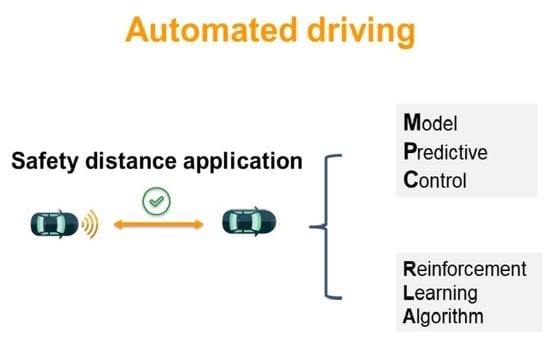
:Many classic control approaches have already proved their merits in the automotive industry. Model predictive control (MPC) is one of the most commonly used methods. However, its efficiency drops off with increase in complexity of the driving environment. Recently, machine learning methods have been considered an efficient alternative to classical control approaches. Even with successful implementation of reinforcement learning in real-world applications, it is still not commonly used compared to supervised and unsupervised learning. In this paper, a reinforcement learning (RL)-based framework is suggested for application in autonomous driving systems to maintain a safe distance. Additionally, an MPC-based control model is designed for the same task. The behavior of the two controllers is compared and discussed. The trained RL model was deployed on a low-end FPGA-in-the-loop (field-programmable gate array in-the-loop). The results showed that the two controllers responded efficiently to changes in the environment. Specifically, the response of the RL controller was faster, at approximately 1.75 s, than that of the MPC controller, while the MPC provided better overshooting performance (approximately 1.3 m/s less) in terms of following the reference speeds. The reinforcement-learning model showed efficient behavior after being deployed on the FPGA with ( ms as a maximum deviation compared to MATLAB Simulink.
1. Introduction
Human perception error is at the top of the significant factors that cause road accidents. Recently, one of the automotive industry’s top priorities has been to provide passengers with the highest level of safety by partially or entirely relieving the driver of responsibilities [1]. Over the past decade, control engineers in the automotive industry have devoted major efforts to improving road transportation by developing and applying advanced control strategies. The advancement of sensing, communication, and processing technologies has resulted in a rapid expansion in the development of advanced driver assistance systems (ADAS) [2]. These systems are designed mainly to assist drivers, either by offering warnings to lessen risk exposure or automating some control functions to relieve a driver of human control [3]. After being tested in highly structured environments and under full supervision, autonomous vehicles have been transitioned to the real world alongside human-driven vehicles. It is anticipated that, in the near future, fully autonomous vehicles would replace humans in the role of drivers. This progress has raised many critical concerns which need to be addressed. Safety-related challenges are at the top of these concerns since it is crucial to ensure that autonomous vehicles are capable of interacting with other vehicles safely. One promising ADAS technology is the adaptive cruise control (ACC) system, which uses data from sensors such as radar to maintain the speed of the vehicle in order to keep a safe distance from other vehicles on the road. A detailed review of ACC systems is provided by [4,5,6]. Studies have demonstrated that the safety systems that have already been implemented in the automotive industry, such as electronic stability control, ACC and lane-following, have reduced the traffic accident rate and consequently increased the safety level [7].
Generally speaking, any control problem can be described as an optimal control problem and several classical control approaches have been used to address the safety problem of autonomous vehicles. In [8], linear temporal logic (LTL) is used to describe the system specifications for adaptive cruise control, where a discrete abstraction of the system serves as the foundation for the controller. However, this solution is computationally expensive as the complexity of the controller synthesis increases exponentially with the dimensions of the system (LTL formula). In [9], the safety constraints are maintained as control barrier functions (CBFs), which penalize the violation of the determined constraints, while the control objective (desired speed) is formulated as control Lyapunov functions. These two sets of functions are structured in quadratic problem (QP) form. Despite the promising performance, the computational loads and the resource requirements are still very high. In addition, finding the control barrier functions is not an easy task. Model predictive control (MPC) is a very well-known control strategy that is used to solve control problems, where it represents the state of the art in real-time optimal control [10] due to its capabilities to deal with multi-input-multi-output (MIMO) systems and handle multiple (soft and hard) constraints using a future prediction strategy. An MPC framework is used to tackle ACC system safety problems and its efficiency in many other autonomous control applications has already been proven [11]. Bageshwar et al. [12] provided an MPC-based control strategy for application to transitional maneuvers. The results showed that the efficiency of the MPC controller in achieving a safe and comfortable driving system depended on the explicit incorporation of collision avoidance and acceleration limits into the formulation of the control problem. Recently, a cooperative adaptive cruise control (CACC) system was introduced. The main idea of the approach is inter-vehicle communication, where all the vehicles within a “cooperative team” know the trajectory of each other. However, a collision can happen when an unexpected maneuver occurs due to a communication problem [13]. Corona et al. [14] successfully implemented a hybrid MPC framework in order to enhance safety by achieving the optimal tracking of a time-varying trajectory. The results confirmed the efficiency of using an MPC controller in an industrial application with computation restrictions. Using an MPC control strategy, multiple control objectives, such as tracking and driver comfort, can be balanced with the cost function by solving the optimal control problem over a finite horizon in a receding fashion [15]. However, MPC design involves many parameters and takes a long time to fine tune, as stated in [16]. In addition, a thorough system dynamics model with high fidelity is required in order to effectively anticipate system states. Solving the optimization problem of high dimensional and non-linear state spaces causes a significant increase in computational loads, which, in turn, affects and impedes real-time implementation, especially with short sample time control. However, linearization is not the best solution to deal with these systems. As a result, implementations of MPC controllers may provide invisible solutions with limited resource computing platforms, such as FPGAs (field-programmable gate arrays) and SOCs (systems-on-chips). Thus, the necessity of developing an alternative control approach that has the capability to deal efficiently with the non-linearity and uncertainty of vehicle dynamics becomes more urgent. In this context, machine-learning algorithms have shown outstanding performance in a wide range of applications in different fields and have recently become an efficient alternative solution to classical control approaches.
Machine learning has been used for many autonomous vehicle applications, including perception and motion planning [17], traffic routing [18], object detection, semantic segmentation [19] and others. Pomerleau’s autonomous land vehicle was one of the earliest research projects to implement machine learning (neural network) for autonomous vehicle control [20]. Generally, machine learning is divided into three main categories: supervised learning, unsupervised learning, and reinforcement learning. Unlike supervised learning and unsupervised learning, implementation of reinforcement-learning algorithms are still a significant challenge. Even with the promising results that have been reported, reinforcement learning is still an emergent field and has not been transitioned to the real world as successfully as supervised and unsupervised learning [21].
Reinforcement learning (RL) is a learning-based algorithm that is used for solving complex sequential decision-making problems by studying the agent’s behavior and its interaction with the environment. RL is structured as Markov decision processes (MDPs), where the agent takes an action within the current state of the environment and consequently receives a reward. The action taken moves the environment to the next state. The objective of an RL agent is to learn an optimal (state-action) mapping policy that maximizes the long-term cumulative rewards it receives over the time. RL depends on trial and error to achieve the optimal policy, with training based on Bellman’s principle of optimality [22,23]. Numerous studies have been conducted on reinforcement learning to address the learning control or sequential decision-making problems occurring within uncertain environments [24]. It is worth mentioning that RL is also known as approximate dynamic programming (ADP) from the perspective of learning control for dynamic systems. An actor-critic reinforcement-learning algorithm is suggested in [25] for addressing the longitudinal velocity tracking control of autonomous land vehicles. The value function and the optimal policy were approximated based on parameterized features that are learned from collected samples so that the actor and critic share the same linear features. The results show the superiority of the approach used over the classical proportional-integral (PI) control. In [26], an RL-based model with energy management is suggested to increase fuel consumption efficiency, where the Q-learning algorithm is implemented to obtain the near-optimal policy. In [27], an RL-based controller is suggested to ensure the longitudinal following of a front vehicle, where a combination of a gradient-descent algorithm and function approximation is employed to optimize the performance of the control policy. This study concluded that, although performance was good, more steps must be taken to address the control policy’s oscillating nature utilizing continuous actions. In [28], a deep reinforcement-learning algorithm was proposed to study the efficiency of RL in handling the problem of navigation within occluded intersections. The solutions discovered by the proposed model highlight various drawbacks of the present rule-based methods and suggest many areas for further investigation in the future. A multi-objective deep reinforcement learning (DQN) [29] approach was suggested for automotive driving in which the agent is trained to drive on multi-lane ways and in intersections. The results show that the learned policy was able to be transferred to a ring-road environment smoothly and without compromising performance.
To better understand the importance of successful implementation of RL algorithms compared to classical MPC, it is important to point out some key differences. MPC is a model-based control strategy that benefits from the accurate dynamics of the plant, which has mainly been developed to solve an optimal control problem of models that have been explicitly formulated for the control problem using a future prediction strategy. In contrast, RL is a learning-based method which has a strong theoretical basis. The efficiency of the model depends on how well the agent is trained within its environment. The high computing demands of MPC for real-time applications raises financial concerns, while offline-trained RL, which uses neural networks, requires relatively minimal computing time during deployment. Additionally, one of the primary advantages of reinforcement learning is its effectiveness in handling high-dimensional environments with complex observations, obtained, for instance, from photos and videos, which are regarded as overly complex for the traditional MPC, which deals with signal measurements. Compared to MPC, the trained policy in a reinforcement-learning model can be viewed as the controller, where the reward function is equivalent to the cost function, while the observations and the actions taken correspond to the measurements and the manipulated variables, respectively [30,31].
This paper seeks to build on studies that have been conducted on reinforcement-learning methods in order to pave the way for more successful RL applications in real-life autonomous vehicle applications and to evaluate their efficiency compared to classical control approaches.
In this paper, two different control models were developed for the purpose of maintaining a safe distance between two vehicles, an MPC-based control system and a reinforcement-learning-based control system. The performance and efficiency of the developed RL-based model were evaluated compared to the behavior of the classical MPC-based model. The two controllers were implemented and tested using the same environment and subjected to the same conditions and constraints.
The paper is structured as follows: In the second section, a brief theoretical background of the optimization problem and the related methods used is provided. In the third section, the design process of the MPC-based and RL-based control models and the implementation steps for the RL model on the FPGA are presented. The implementations and the results obtained are discussed in the fourth section. Finally, the conclusions are summarized in the last section.
2. Materials and Methods
2.1. General Optimization Problem
Optimization is considered essential in a variety of applications in different areas, including engineering, science and business. The goal of the optimization process differs from one application to another based on the nature of the task itself. Generally, optimization provides improvements in different respects with the aim of minimizing power consumption and cost or maximizing performance, outputs and profits. The value and necessity of the optimization process mainly derives from the complexity of real-world problems and limitations regarding resources, time and computational capabilities. This means that finding solutions to optimally manage and use these resources is an essential topic for research. As a result, it is not an overstatement to say that optimization is needed in each and every real-world application.
Mathematically speaking, any optimization problem consists of an objective function, decision variables and constraints. The objective function needs to be minimized or maximized and must be subjected to constraints, which can be soft and/or hard. The standard mathematical form for most optimization problems can be described as
where is the objective function, are inequality constraints, are equality constraints, N is the number of objective functions, J is the number of inequality constraints and L is the number of equality constraints. The objective function can be linear or non-linear and, similarly, the constraints can be linear, non-linear or even mixed. The components of the vector are called decision variables and can be discrete or continuous variables. The inequality constraints can also be written in the form () and the cost function can be formulated as a maximization problem
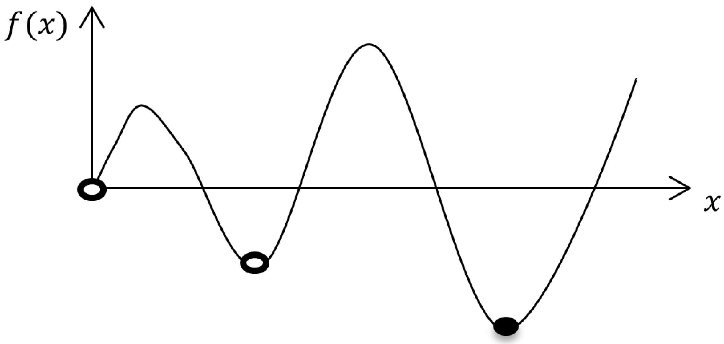
The optimization problem can be classified based on two factors: the number of objective functions and the number of constraints. In terms of the number of objective functions, it can be divided into a single objective where N = 1 and a multi objective where . In terms of number constraints, the optimization problem is divided into unconstrained (j = l = 0), inequality constrained (l = 0 and ) and equality constrained (j = 0 and ) optimization problems. It is worth pointing out that, if both the objective function and the constraints are linear, then the optimization problem is called a linear programming problem. In the case where both the objective function and constraints are non-linear, the problem becomes a non-linear optimization problem. The problem is called quadratic programming (QP) when the objective is a linear–quadratic function and the constraints are affine (linear combinations). In certain objective functions, we could have a local minimum or global minimum. The point is called the local minimum if the value of the function at this point is equal to or smaller than its values at nearby points. When the value of the function at this point is equal to or smaller than its values at the feasible points, the point is called the global minimum. Figure 1 shows three local minimum points and one global minimum point. Global optimization problems are usually more complex and challenging [32].
2.2. Model Predictive Controller
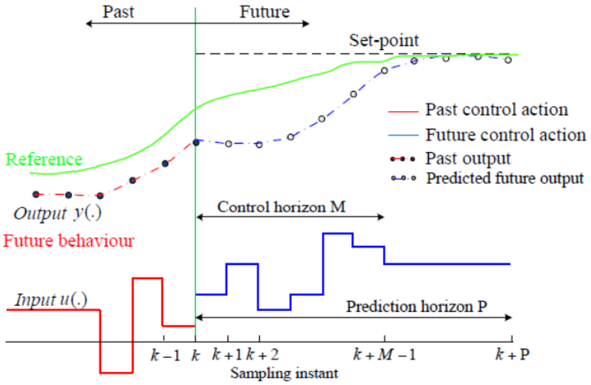
MPC is a very well-known classical control strategy that is used in a variety of applications. An MPC controller solves an online constrained optimization problem, which is mainly a quadratic problem (QP). MPC uses an optimizer to ensure that the output of the plant model follows the reference target. Figure 2 shows the control loop of the MPC controller. The goal of the MPC controller is to minimize the cost function and satisfy the system constraints, such as acceleration and physical boundaries. MPC uses a future prediction strategy to output its control actions, where it looks forward to the future and uses its internal plant model to simulate different scenarios based on the current state. Here the optimizer comes into the picture by choosing the optimal scenario. The optimal predicted scenario is the one that achieves the minimum error compared to the reference target (Figure 3). Figure 4 shows the designing parameters of the MPC controller, where is the sample time, which determines the rate at which the MPC controller executes its algorithm, k is the current sampling step, the prediction horizon (P) represents the time over which the controller looks forward into the future to make predictions, and the control horizon (M) represents the possible control steps to the (k+P) time step. The MPC controller solves the optimization problem at each time step, which makes the process computationally expensive. In the design process, and in order to balance performance and computational load, it is important to consider that, by determining a long time-step interval, the MPC will not be able to respond in time and, while the response will be faster for a small time step, the computational load will significantly increase. The control horizon should be chosen in a way that covers the dynamic changes in the system. The response behavior of the MPC is significantly affected by the first two control moves; therefore, a large control horizon will only increase the computation complexity [33].
2.3. Reinforcement Learning
Reinforcement learning is a category of machine learning that is formulated as Markov decision processes (MDPs). An MDP system consists of an agent (decision-maker), a set of actions (T), a set of states (S), a transaction function (A) and a reward function (R). At each time step, the agent takes an action based on the current state and the environment is transitioned to a new state , where the agent receives a reward . The main goal is maximizing the total cumulative reward, which simply represents the sum of the expected returns at each time step. Figure 5 shows the MDP process. For continuous systems, the final time step T = ∞; therefore, the total reward cannot be calculated. To solve this problem, the concept of discounted reward is used and the goal, in turn, is to maximize the discounted total reward. The main idea behind this concept is to minimize the effect of future returns on the actions taken in a way that causes the action taken to be greatly influenced by the immediate reward compared to future ones. Equation (3) represents the concept of the total discounted reward.
where G is the total reward and is the discount factor which is chosen to be in the range [0–1].
The function that maps the probabilities of selecting each action at a specific state is called the policy (). The function that evaluates how good it is for the agent to be in a specific state under the policy () is called the state-value function (), while the function that evaluates how good it is for the agent to select a specific action under policy () at a given state is called the Q-function or the action-value function (). The optimal policy () corresponds to the optimal Q-function () and the optimal state-value function () [34,35]. Based on the way the agent learns the policy and/or the value function estimates, reinforcement learning is categorized into three main methods: policy-based methods, value-based methods and actor-critic methods [36,37,38]. All the RL methods follow the same strategy of evaluating the agent’s behavior; however, the fundamental distinction between them relates to where the optimality resides. Q-learning and deep Q-learning are the most common value-based methods. In Q-learning, the Q-values for each pair (state, action) are stored in a Q-table and the agent determines the optimal policy by learning how to find the optimal Q-value. In reinforcement learning, the agent may exploit its knowledge by selecting an action that is known to provide a positive reward in order to maximize the total reward. On the other hand, the agent may take the risk of exploring unknown actions, which may lead to a lower reward or to discovering actions that provide a higher reward compared to the current best-valued action. Managing the exploration-exploitation trade-off is considered a critical challenge for the RL algorithm and an -greedy approach is one of the most commonly used strategies to overcome this challenge. In this strategy, the exploration rate () refers to the probability of exploring the environment rather than exploiting it, meaning that the agent will either choose an action randomly with probability () or will be greedy by selecting the highest valued action with probability (1-). Since the agent at the beginning knows nothing about the environment, the exploration rate () is usually initialized to be one, so the agent starts by exploring the environment. With progress of training, the agent learns more about the environment and should conduct more exploitation, which can be achieved by gradually decreasing the probability of exploration () by a specific rate at the beginning of every new episode. After taking the action, the agent observes the next state, obtains the gained reward and updates the Q-table. With increase in the state space size the efficiency of the Q-learning algorithm drops off due to its iteration strategy and the large number of pairs (state-action) that need to be stored in the Q-table. The deep Q-learning algorithm overcomes this problem by using a deep neural network as a function approximation to estimate the optimal Q-value instead of the value iteration strategy. Instead of learning the optimal policy based on the cumulative reward, the policy-based method directly optimizes the policy itself by parametrizing the policy and determining the parameters in a way that maximize the objective function of the policy. The advantages of the value-based and the policy-based methods are combined in the actor-critic method, where two different approximators are used to determine and update the parameters of the policy and the actions-value function. The deep deterministic policy gradient (DDPG) approach is one of the most common actor-critic methods. The DDPG algorithm uses two neural network-based approximators, the critic and the actor. The actor deterministically approximates the best action for the given state, while the critic evaluates the action taken [39,40].
2.4. Design of the Controllers Models
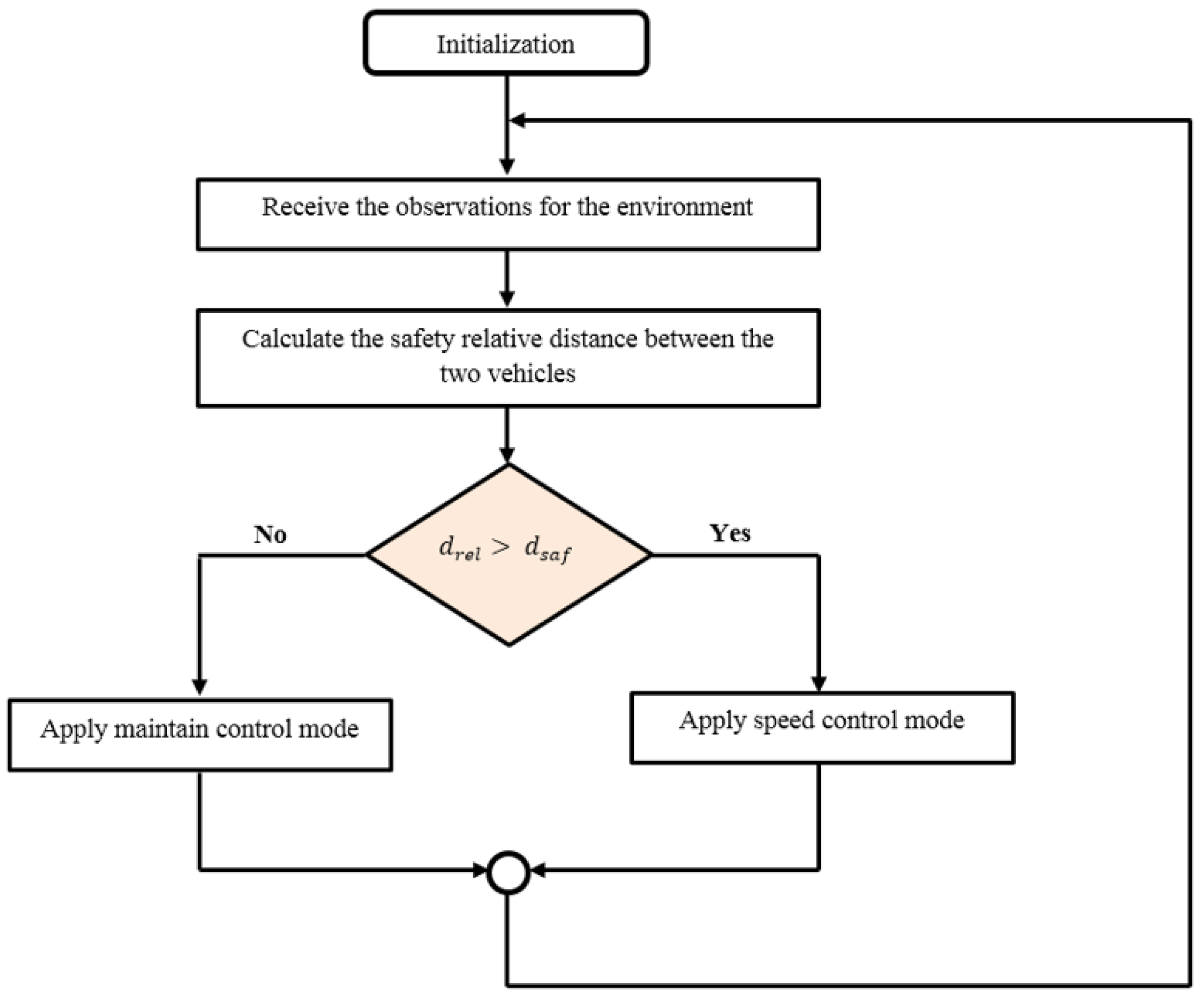
The two controllers are designed to respond to the environment changes using two control modes: the speed and maintain modes. In the case where the relative distance () between the two vehicles (ego vehicle and leading vehicle) is greater than the reference safety distance (), the controller applies the speed mode that makes the ego vehicle drive at the reference velocity. In the case where the relative distance is less than the safety distance, the controller switches to the maintain mode and the vehicle drives at the speed of the leading vehicle to keep a safe distance (Figure 6).
2.4.1. Design of the MPC Controller
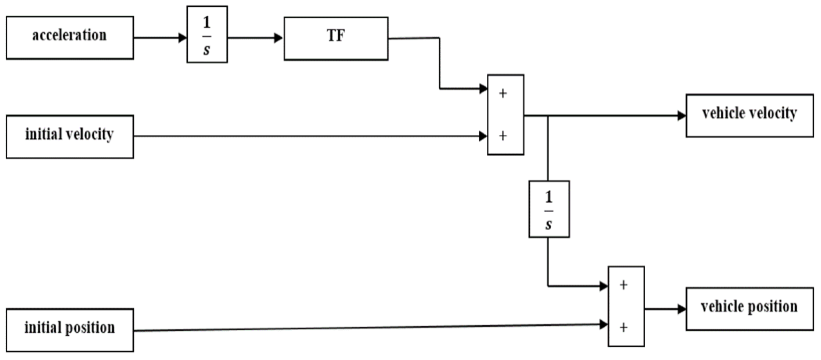
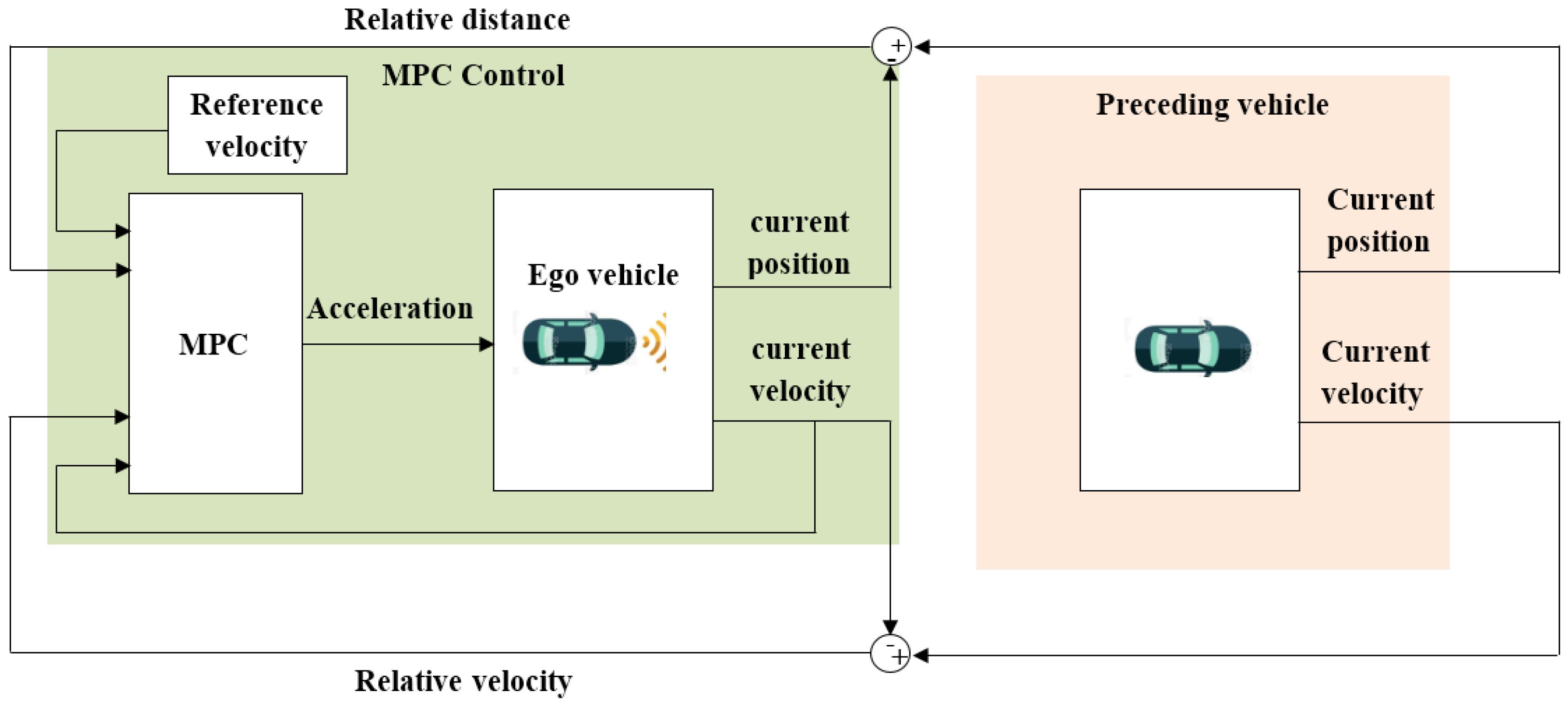
As the MPC controller is a model-based control strategy and depends on the feedback coming from its internal plant, the first step in the design process is to design the model that describes the relation between the longitudinal velocity and the acceleration of the vehicle. This relation is subjected to the dynamics that describe the relation between the engine throttle system and the resistance of the vehicle to the change in direction or velocity (vehicle inertia). The throttle system regulates how much air and fuel mixture reaches the engine cylinders using a control valve. By increasing the opening angle of the control valve, more fuel mixture enters the engine, which, in turn, increases the vehicle speed. Equation 4 describes this relation, where TF is the transfer system that approximates the dynamics between the throttle system and the vehicle inertia. Figure 7 shows the subsystem block in MATLAB Simulink, which describes the transfer function in connection with the velocity, acceleration and position of the vehicle. After designing the plant model, the next step is to determine the input/output signals and the design parameters of the control system (Figure 8 and Table 1). The measured outputs are used for state estimation, while the manipulated variables are the optimal control actions. The MPC design parameters and the control constraints are presented in Table 2. Figure 9 shows the overall workflow of the MPC-based control system.
2.4.2. Designing and Training the Reinforcement-Learning-Based Controller
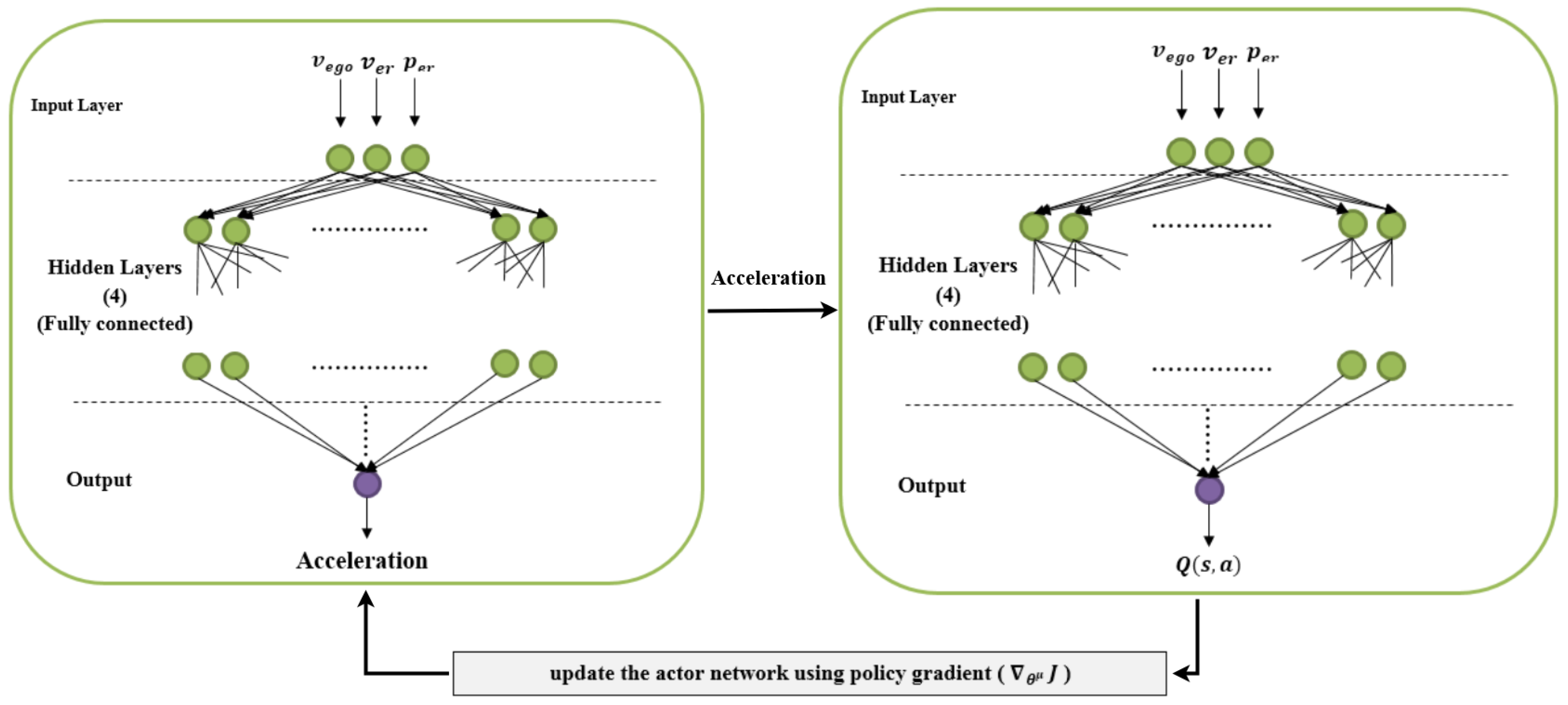
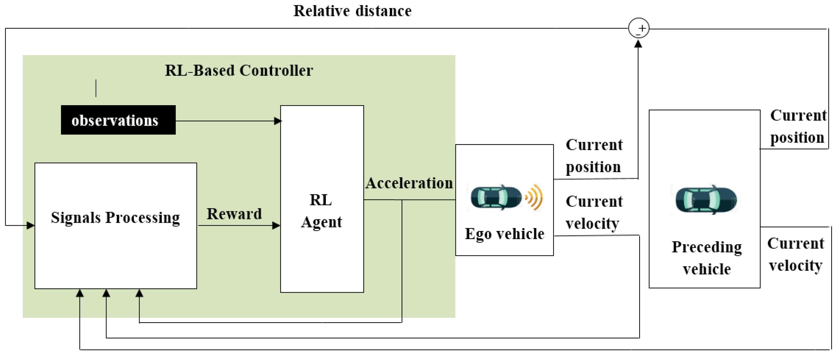
In this study, the deep deterministic policy gradient algorithm is used to design the reinforcement leaning controller. As mentioned earlier, this algorithm uses two different deep-learning-based approximators, the actor and the critic. The design process went through several steps, starting from preparing the environment, designing the neural networks of the actor and critic, creating and training the agent, and, finally, running, testing and validating the model. The observations of the environment are determined to be the vehicle velocity (), the velocity error () and the integral velocity error (). The velocity error represents the difference between the reference and the vehicle velocity. The acceleration constraint is determined to be in the same range as that of the MPC controller, [−3, 3] m. Figure 10 shows the neural network structure of the actor-critic approximators.
In detail, the critic network consists of two input layers, four hidden layers and one output layer. The first input layer is structured with three neurons to receive the three observations from the environment, while the second input layer is structured with one node to receive the action from the actor network. Each hidden layer consists of 50 neurons and ReLU is used as an activation function between the layers. The output layer consists of one neuron to output the estimated Q-value. The actor network consists of one input layer with three neurons to receive the observations, five hidden layers, each one structured with 50 neurons, and a ReLU activation function between the layers. Figure 11 shows the overall workflow of the RL-based control system.
2.4.3. Training Algorithm
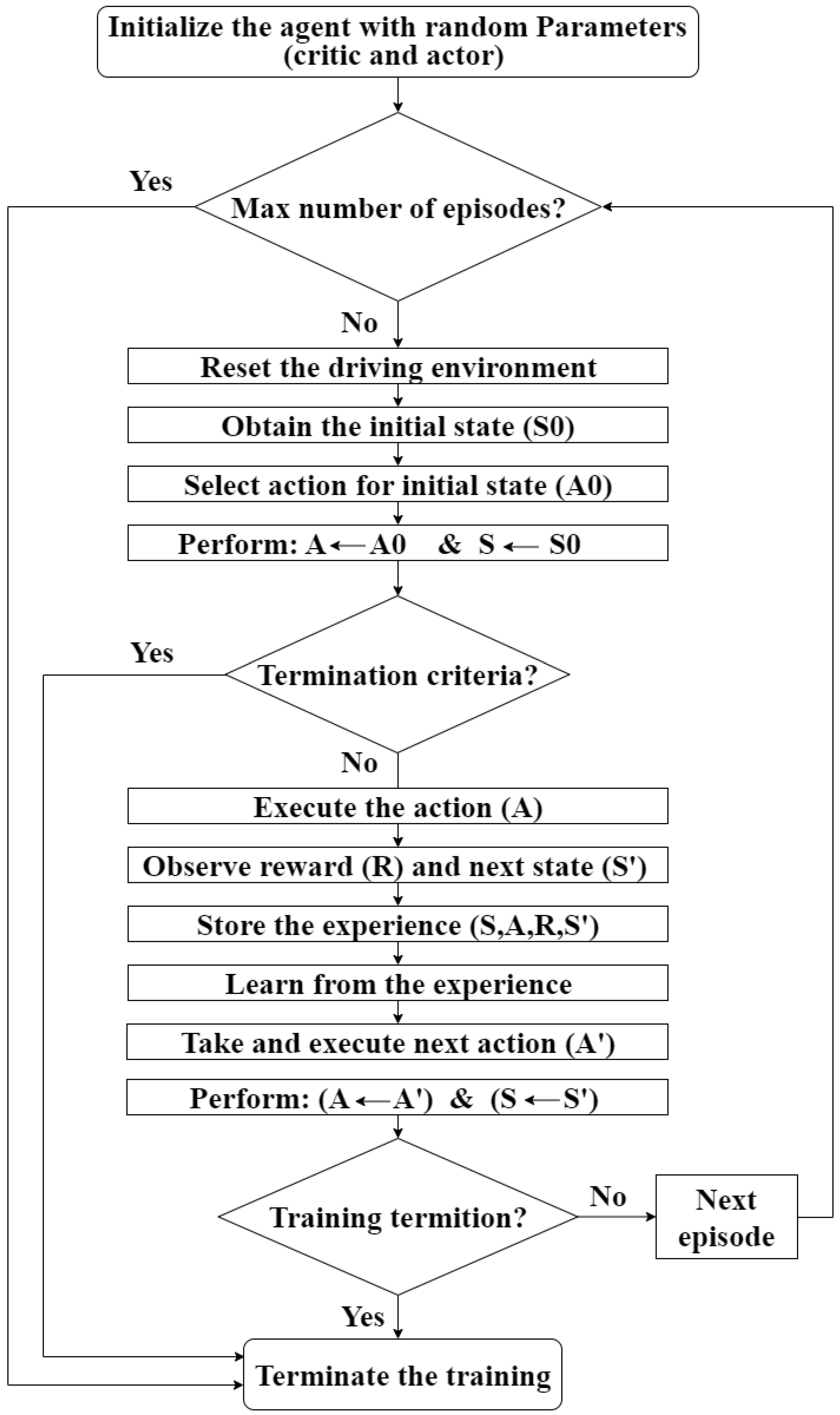
The goal of the training is finding the optimal policy which achieves the highest cumulative rewards. During the training, the parameters of the policy are updated based on the following algorithm: taking action, getting the reward, and updating the policy. This cycle continues until the trained agent learns to take the best action that achieves the highest long-term reward at each state. The training options are determined, including the maximum number of episodes, the number of steps per episode and the stop training criteria. Assuming S and A represent the state and the action, respectively, the training algorithms can be summarised as shown in Figure 12.
2.4.4. SOC Implementations and Verification of RL Model
As the reinforcement-learning algorithm depends on trial and error, it was safer to first test the design using the MATLAB Simulink, before implementation on the real SOC. For this purpose, multiple simulations were performed and the final trained policy that met the requirements was taken to the next step to be deployed on the target FPGA. The suggested RL-based control model was deployed on a low-end SOC (ZedBoard). The deployment process went through several steps (see Figure 13). In the first step, the trained policy was extracted from the trained agent (the Simulink model) and represented in C code generated using the MATLAB embedded coder. The generated code accepts the environment observations as inputs, and outputs the optimal action for the current state based on the trained policy. In the next step, the hardware configurations were prepared in order to enable communication between the SOC and MATLAB Simulink. The deployment was performed by downloading and running the generated code on the target SOC. Running the model on Zedboard goes through the following cycle: SOC receives the signals from MATLAB Simulink through the communication channel, executes the algorithm, outputs a control action (acceleration or deceleration), and then sends it to the Simulink model to update the state of the driving environment.
3. Results and Discussion
In the first part of this section, the performance of the RL model is evaluated and compared to the performance of the MPC model. In the second part of the section, the deployment of the RL-based model on SOC is discussed and evaluated compared to the Simulink results. The efficiency of the models is determined based on different metrics: the ability to follow the environment changes, the response time, overshooting, and the ability of the controller to switch between the two control modes (the speed and maintain modes) in a way that the vehicle will either keep a safe distance by following the preceding vehicle or follow the reference speed based on the current state of the environment.
3.1. MATLAB Simulink
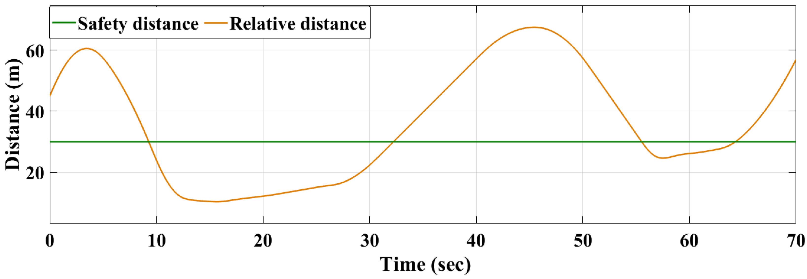
Figure 14, Figure 15 and Figure 16 present the obtained results of the MPC model while Figure 17, Figure 18 and Figure 19 present the obtained results of RL model. Figure 14 and Figure 17 show the behavior of the MPC and RL-based controllers, respectively, and their response to different driving scenarios. Figure 15 and Figure 18 show the relative distance between the two vehicles compared to the reference safety distance. Figure 16 and Figure 19 show the change in the preceding vehicle’s velocity, the reference velocity and the response of the ego vehicle to the outputs of the controllers.
3.1.1. MPC Controller
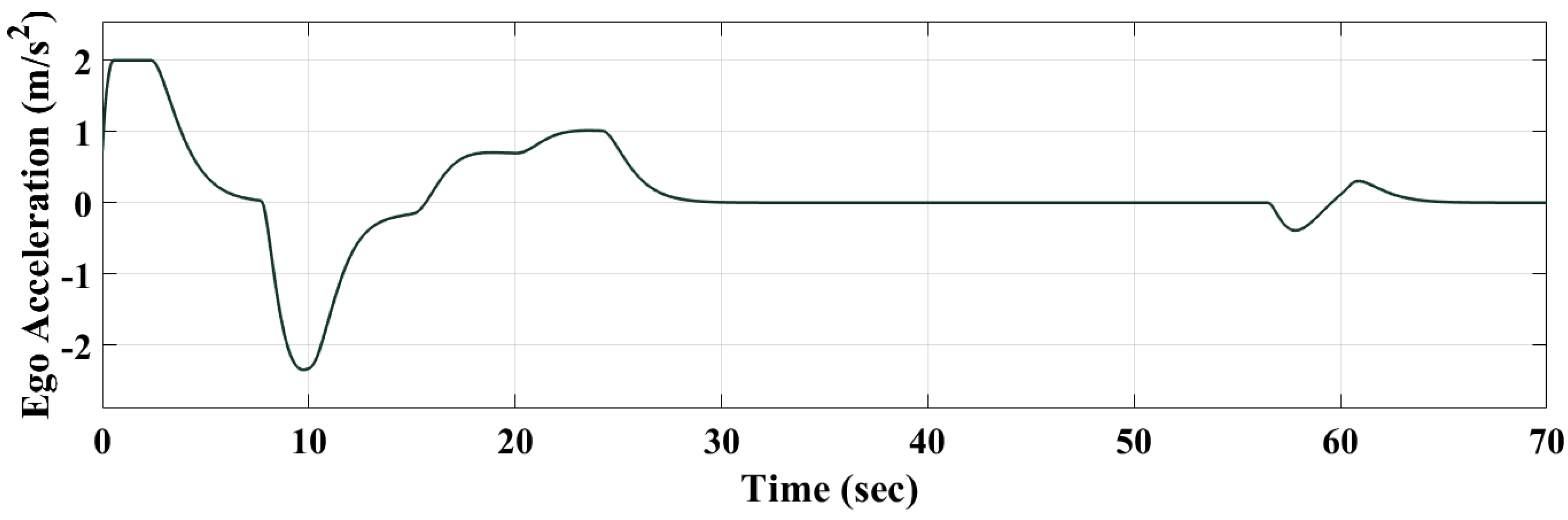
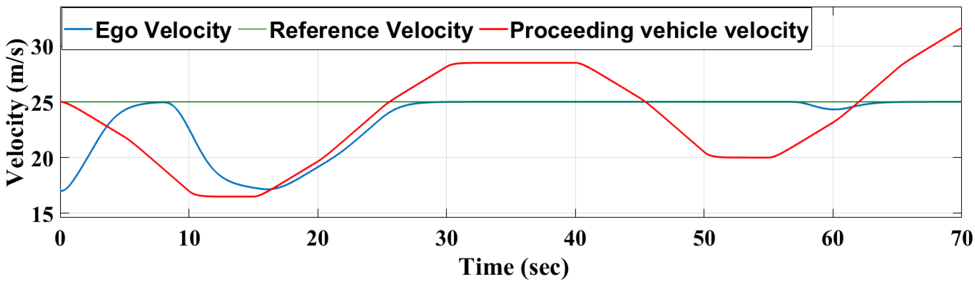
Figure 15 shows that, in the first 10 seconds, the relative distance between the two vehicles is greater than the safety distance; the MPC controller response is based on the speed control mode, where it successfully drives the ego vehicle to follow the reference velocity (Figure 16). Between 12 to 28 s, the relative distance is less than the safety distance, the MPC controller switches to “maintain” control mode and the ego vehicle changes its speed in order to follow the minimum speed of the preceding vehicle. The detailed behavior of the MPC during this period of time (0 to 28 s) shows that, in the first three seconds, the MPC controller outputs a near maximum acceleration (Figure 14) since the relative distance is much higher than the safety distance and the ego vehicle follows the reference speed. On the other hand, with the continuous decrease in the velocity of the preceding vehicle and, consequently, the relative distance, the MPC begins to gradually reduce the acceleration. At second 10, the relative distance becomes very close to the safety distance. The MPC controller switches to the “maintain” control mode and responds in a way that drives the vehicle in the direction of following the speed of the preceding vehicle. At second 28, the MPC controller switches back to “speed” mode and the ego vehicle follows the reference speed until second 58, regardless of the (maximum or minimum) speed of the preceding vehicle, since the relative distance is greater than the safety distance.
3.1.2. Reinforcement-Learning Control Model
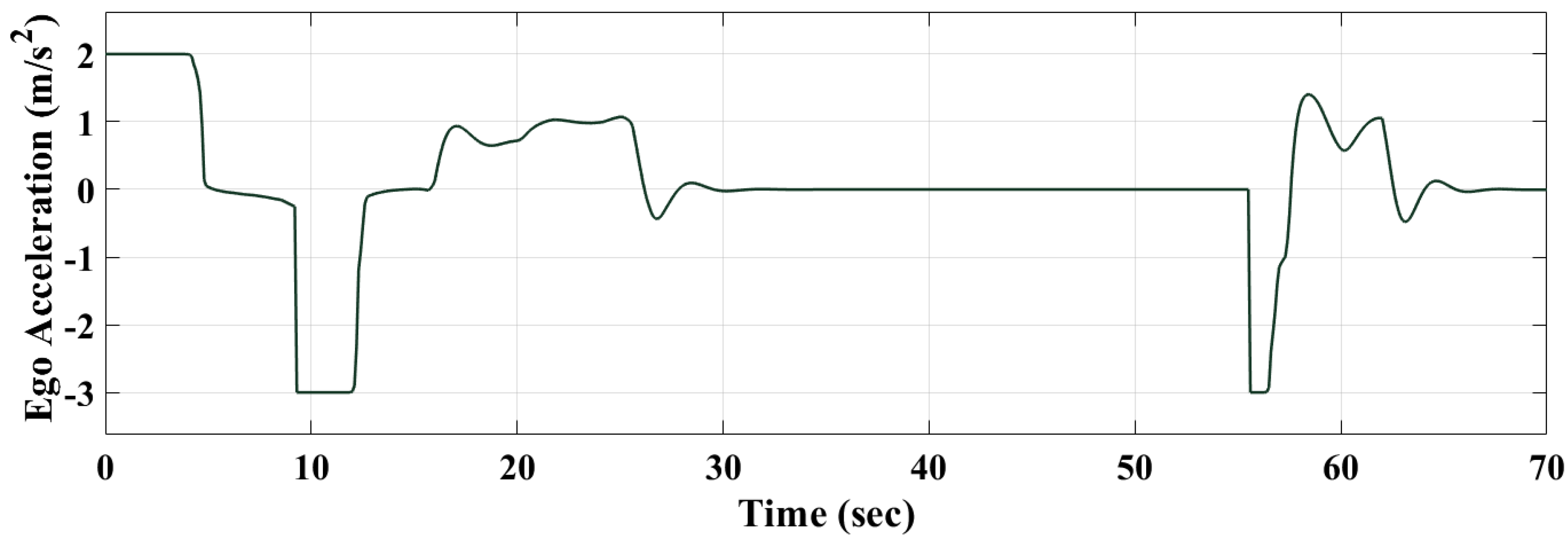
Figure 17, Figure 18 and Figure 19 show that the RL-based controller is able to switch between “speed” and “maintain” control modes efficiently. The controller drives the ego vehicle to follow the reference speed between 0 to 10 s since the relative distance is greater than the safety distance. Then it successfully switches to “maintain” control mode when the relative distance becomes very close to or less than the safety distance between 10 to 28 s. From 31 to 56 s, the relative distance is greater than the safety distance and the RL controller switches back to the “speed” control mode, where the ego vehicle follows the reference speed.
3.1.3. Performance Comparison
The results show that both controllers responded efficiently to the changes in the environment based on the control modes and the design specifications. In detail, at the beginning, the RL controller drove the vehicle from the initial state to the reference velocity in approximately 4.5 s, while it took around 6.2 s in the case of the MPC controller. The results also show that the RL controller was able to follow and respond to changes in the environment faster than the MPC controller—it took approximately 4.6 s to reach the preceding vehicle speed after changing to “maintain” mode with the RL controller, while it took approximately 6.4 s in the case of the MPC controller. Similarly, the results show stable behaviour of the RL model, which responded faster to the other environment changes, driving the vehicle at the reference speed at 26 s after switching back to the speed control mode, while the MPC controller reached the reference speed at 28.5 s. The RL-based model improved the response time by 1.75 s on average.
On the other hand, the behavior of the RL controller showed higher overshooting in terms of following the reference speed compared to the MPC behavior, especially against the initial state, where the maximum overshooting was approximately 1.3 m/s. In conclusion, the results demonstrate the advantage of the reinforcement-learning model in terms of the ability to predict and follow changes in the state of the environment faster than the MPC controller. This result is compatible with the fact that solving the optimization problem using a trained neural network is faster than solving an online quadratic problem at each time step (MPC controller). On the other hand, the results demonstrate the advantage of MPC control in terms of producing less overshooting behaviour in all switching points.
3.2. RL-Model on SOC
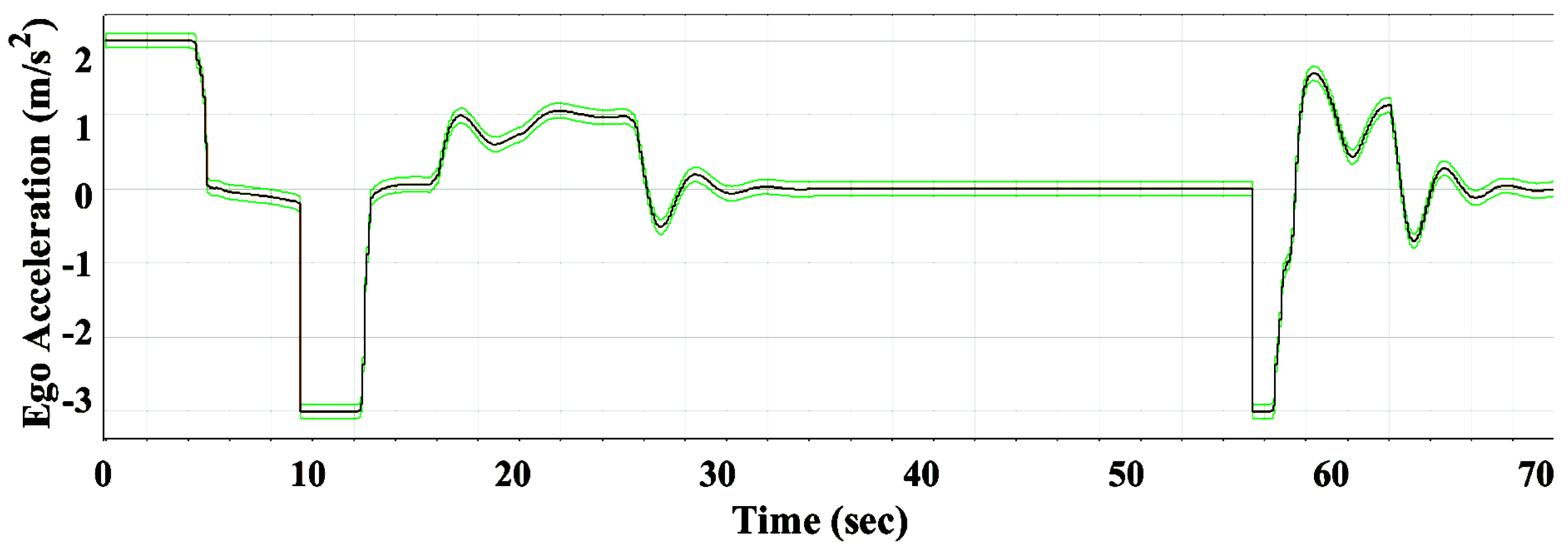
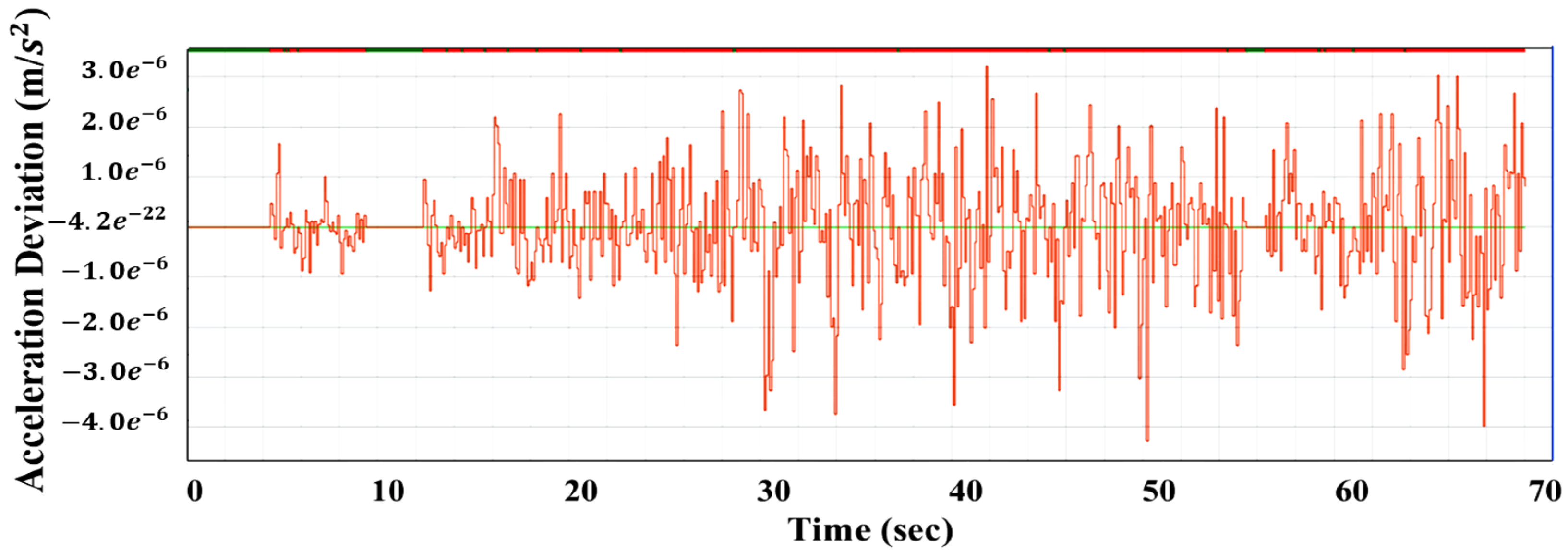
The performance of the RL controller after being implemented on SOC was evaluated compared to its performance on MATLAB Simulink. The compression was analyzed in terms of tolerance error, which was determined to be 0.2 m/s maximum. The results shown in Figure 20 indicate that the response of the RL controller was within the determined tolerance range. Figure 21 represents the detailed deviations where the maximum was ( m/s). These results demonstrate the success of the deployment of the proposed RL controller on SOC, which also, in turn, indicates the effectiveness of the approach employed for extracting the optimal policy that is trained and validated using MATLAB Simulink.
4. Conclusions
In contrast to classical control strategies, whose efficiency depends strictly on the design parameters, the reinforcement-learning algorithm provides an efficient generalizable model and higher stable control using a very well-trained agent that is exposed to all possible scenarios within the environment.
In this paper, a reinforcement-learning-based control strategy was suggested for the task of maintaining a safe distance in an automated driving system.
The efficiency of the reinforcement-learning algorithm was studied as an alternative approach to the classical MPC control. The performance of the suggested model was evaluated compared to the performance of an MPC controller that was designed for the same task. Additionally, the RL model was deployed on a low-end FPGA/SOC after being verified in MATLAB Simulink. The results obtained show the superiority of the reinforcement-learning algorithm over the MPC in terms of the ability to predict, follow and respond faster to environment changes. The RL model provided stable behaviour against the changes in the environment, improving the response time by 1.75 s on average. On the other hand, the MPC controller outperformed the RL-based controller performing with less overshooting (approximately 1.3 m/s less), which demonstrates the advantage of MPC control in terms of overshooting behavior. After verifying the reinforcement-learning model, the trained policy was extracted and successfully deployed on FPGA. The obtained results showed stable behaviour of the RL model after being implemented on FPGA compared to the Simulink behaviour, where its response was within the tolerance range (0.2 ms) and the maximum deviation was ( m/s). In conclusion, developing a reinforcement-learning-based control strategy for highly complex environments can be considered a promising and efficient solution to address the disadvantages of classical control approaches.
Author Contributions
Conceptualization, A.R. and J.V.; methodology, A.R. and J.V.; formal analysis, A.R. and J.V.; writing—original draft preparation, A.R. and J.V.; writing—review and editing, A.R. and J.V. All authors have read and agreed to the published version of the manuscript.
Funding
This research received no external funding.
Informed Consent Statement
Not applicable.
Conflicts of Interest
The authors declare no conflict of interest.
Abbreviations
The following abbreviations are used in this manuscript:
| ACC | Adaptive Cruise Control |
| RL | Reinforcement Learning |
| ADAS | Advanced Driver Assistance Systems |
| CACC | Cooperative Adaptive Cruise Control |
| DQN | Deep Q-Learning |
| FPGA | Field-Programmable Gate Array |
| LTL | Linear Temporal Logic |
| MDP | Markov Decision Process |
| MIMO | Multi-Input-Multi-Output |
| MPC | Model Predictive Control |
| QP | Quadratic Problem |
| SOC | System-on-Chip |
References
- Magdici, S.; Althoff, M. Adaptive cruise control with safety guarantees for autonomous vehicles. IFAC 2017, 10, 5774–5781. [Google Scholar] [CrossRef]
- Ziebinski, A.; Cupek, R.; Grzechca, D.; Chruszczyk, L. Review of advanced driver assistance systems (ADAS). In AIP Conference Proceedings; AIP Publishing LLC: Melville, NY, USA, 2017; Volume 1906. [Google Scholar]
- Ioannou, P.; Wang, Y.; Chang, H. Integrated Roadway/Adaptive Cruise Control System: Safety, Performance, Environmental and Near Term Deployment Considerations; California PATH Research Report UCB-ITS-PRR, California PATH Program, Institute of Transportation Studies, University of California: Berkeley, CA, USA, 2007. [Google Scholar]
- Xiao, L.; Gao, F. A comprehensive review of the development of adaptive cruise control systems. Veh. Syst. Dyn. 2010, 48, 1167–1192. [Google Scholar] [CrossRef]
- ISO 15622; Intelligent Transport Systems—Adaptive Cruise Control Systems—Performance Requirements and Test Procedures. ISO: Geneva, Switzerland, 2010. Available online: https://www.iso.org/standard/71515.html (accessed on 20 November 2022).
- Moon, S.; Moon, I.; Yi, K. Design, tuning, and evaluation of a full-range adaptive cruise control system with collision avoidance. Control Eng. Pract. 2009, 17, 442–455. [Google Scholar] [CrossRef]
- Rieger, G.; Scheef, J.; Becker, H.; Stanzel, M.; Zobel, R. Active safety systems change accident environment of vehicles significantly-a challenge for vehicle design. In Proceedings of the 19th International Technical Conference on the Enhanced Safety of Vehicles (ESV), Washington, DC, USA, 6–9 June 2005. [Google Scholar]
- Nilsson, P.; Hussien, O.; Chen, Y.; Balkan, A.; Rungger, M.; Ames, A.; Grizzle, J.; Ozay, N.; Peng, H.; Tabuada, P. Preliminary results on correct-by-construction control software synthesis for adaptive cruise control. In Proceedings of the IEEE Conference on Decision and Control, Piscataway, NJ, USA, 15 December 2014; pp. 816–823. [Google Scholar]
- Ames, A.D.; Grizzle, J.W.; Tabuada, P. Control barrier function based quadratic programs with application to adaptive cruise control. In Proceedings of the IEEE 53rd Annual Conference on Decision and Control, Los Angeles, CA, USA, 15 December 2014; pp. 6271–6278. [Google Scholar]
- Diehl, M.; Ferreau, H.J.; Haverbeke, N. Efficient Numerical Methods for Nonlinear MPC and Moving Horizon Estimation. In Nonlinear Model Predictive Control. Lecture Notes in Control and Information Sciences; Springer: Berlin, Germany, 2009; Volume 384, pp. 391–417. [Google Scholar]
- Stanger, T.; del Re, L.; Stanger, T.; del Re, L. A model predictive cooperative adaptive cruise control approach. In Proceedings of the American Control Conference, Washington, DC, USA, 17–19 June 2013. [Google Scholar]
- Bageshwar, V.L.; Garrard, W.L.; Rajamani, R. Model predictive control of transitional maneuvers for adaptive cruise control vehicles. IEEE Trans. Veh. Technol. 2004, 53, 1573–1585. [Google Scholar] [CrossRef]
- Dey, K.C.; Yan, L.; Wang, X.; Wang, Y.; Shen, H.; Chowdhury, M.; Yu, L.; Qiu, C.; Soundararaj, V. A Review of Communication, Driver Characteristics, and Controls Aspects of Cooperative Adaptive Cruise Control (CACC). IEEE Trans. Intell. Transp. Syst. 2016, 17, 491–509. [Google Scholar] [CrossRef]
- Corona, D.; Lazar, M.; De Schutter, B. A hybrid MPC approach to the design of a Smart adaptive cruise controller. In Proceedings of the IEEE International Symposium on Computer Aided Control System Design, San Francisco, CA, USA, 13–15 April 2009. [Google Scholar]
- Wei, S.; Zou, Y.; Zhang, T.; Zhang, X.; Wang, W. Design and Experimental Validation of a Cooperative Adaptive Cruise Control System Based on Supervised Reinforcement Learning. Appl. Sci. 2018, 8, 1014. [Google Scholar] [CrossRef] [Green Version]
- Kianfar, R.; Augusto, B.; Ebadighajari, A.; Hakeem, U.; Nilsson, J.; Raza, A.; Papanastasiou, S. Design and Experimental Validation of a Cooperative Driving System in the Grand Cooperative Driving Challenge. IEEE Trans. Intell. Transp. Syst. 2012, 13, 994–1007. [Google Scholar] [CrossRef] [Green Version]
- Pfeiffer, M.; Schaeuble, M.; Nieto, J.; Siegwart, R.; Cadena, C. From perception to decision: A data-driven approach to end-to-end motion planning for autonomous ground robots. In Proceedings of the 2017 IEEE International Conference on Robotics and Automation (ICRA), Singapore, 29 May–3 June 2017; pp. 1527–1533. [Google Scholar]
- Lamouik, I.; Yahyaouy, A.; Sabri, M.A. Deep neural network dynamic traffic routing system for vehicle. In Proceedings of the 2018 International Conference on Intelligent Systems and Computer Vision (ISCV), Fez, Morocco, 2–4 April 2018. [Google Scholar]
- Girshick, R.; Donahue, J.; Darrell, T.; Malik, J. Rich feature hierarchies for accurate object detection and semantic segmentation. In Proceedings of the IEEE Conference on Computer Vision and Pattern Recognition, Columbus, OH, USA, 23–28 June 2014; pp. 580–587. [Google Scholar]
- Amari, S. The Handbook of Brain Theory and Neural Networks; MIT Press: Cambridge, MA, USA, 2003. [Google Scholar]
- Ernst, D.; Glavic, M.; Capitanescu, F.; Wehenkel, L. Reinforcement learning versus model predictive control: A comparison on a power system problem. IEEE Trans. Syst. Man Cyb. 2008, 39, 517–529. [Google Scholar] [CrossRef] [PubMed] [Green Version]
- Lin, Y.; McPhee, J.; Azad, N.L. Comparison of deep reinforcement learning and model predictive control for adaptive cruise control. IEEE Trans. Intell. Veh. 2020, 6, 221–231. [Google Scholar] [CrossRef]
- Sutton, R.S.; Barto, A.G.; Sutton, R.S.; Barto, A.G. Reinforcement Learning: An Introduction; MIT Press: Cambridge, MA, USA, 2018. [Google Scholar]
- Xu, X.; Zuo, L.; Huang, Z. Reinforcement learning algorithms with function approximation: Recent advance and applications. Inf. Sci. 2014, 216, 1–31. [Google Scholar] [CrossRef]
- Huang, Z.; Xu, X.; He, H.; Tan, J.; Sun, Z. Parameterized Batch Reinforcement Learning for Longitudinal Control of Autonomous Land Vehicles. IEEE Trans. Syst. Man. Cybern. Syst 2019, 49, 730–741. [Google Scholar] [CrossRef]
- Liu, T.; Zou, Y.; Liu, D.X.; Sun, F.C. Reinforcement Learning of Adaptive Energy Management With Transition Probability for a Hybrid Electric Tracked Vehicle. IEEE Trans. Ind. Electron. 2015, 62, 7837–7846. [Google Scholar] [CrossRef]
- Desjardins, C.; Chaib-Draa, B. Cooperative adaptive cruise control: A reinforcement learning approach. IEEE Trans. Intell. Transp. Syst. 2011, 12, 1248–1260. [Google Scholar] [CrossRef]
- Isele, D.; Rahimi, R.; Cosgun, A.; Subramanian, K.; Fujimura, K. Navigating occluded intersections with autonomous vehicles using deep reinforcement learning. In Proceedings of the 2018 IEEE International Conference on Robotics and Automation (ICRA), Brisbane, Australia, 21–25 May 2018; pp. 2034–2039. [Google Scholar]
- Li, C.; Czarnecki, K. Urban driving with multi-objective deep reinforcement learning. Proc. Int. Jt. Conf. Auton. Agents Multiagent Syst. AAMAS 2019, 1, 359–367. [Google Scholar]
- Vajedi, M.; Azad, N.L. Ecological adaptive cruise controller for plug-in hybrid electric vehicles using nonlinear model predictive control. IEEE Trans. Intell Transp. Syst. 2015, 10, 113–122. [Google Scholar] [CrossRef]
- Lee, J.; Balakrishnan, A.; Gaurav, A.; Czarnecki, K.; Sedwards, S. W ise M ove: A Framework to Investigate Safe Deep Reinforcement Learning for Autonomous Driving. In Proceedings of the 16th International Conference on Quantitative Evaluation of Systems, Glasgow, UK, 10–12 September 2019. [Google Scholar]
- Venter, G. Review of Optimization Techniques; John Wiley & Sons Ltd.: Chichester, UK, 2010. [Google Scholar] [CrossRef] [Green Version]
- Reda, A.; Bouzid, A.; Vásárhelyi, J. Model Predictive Control for Automated Vehicle Steering. Acta Polytech. Hung. 2020, 17, 163–182. [Google Scholar] [CrossRef]
- Puterman, M.L. Markov Decision Processes: Discrete Stochastic Dynamic Programming; John Wiley & Sons: New York, NY, USA, 2014. [Google Scholar]
- Howard, R.A. Dynamic Programming and Markov Processes; MIT Press: Cambridge, MA, USA, 1960. [Google Scholar]
- Arulkumaran, K.; Deisenroth, M.P.; Brundage, M.; Bharath, A.A. Deep reinforcement learning: A brief survey. IEEE Signal Process. Mag. 2017, 34, 26–38. [Google Scholar] [CrossRef] [Green Version]
- Lillicrap, T.P.; Hunt, J.J.; Pritzel, A.; Heess, N.; Erez, T.; Tassa, Y.; Silver, D.; Wierstra, D. Continuous control with deep reinforcement learning. arXiv 2022, arXiv:1509.02971. [Google Scholar]
- Mnih, V.; Kavukcuoglu, K.; Silver, D.; Rusu, A.A.; Veness, J.; Bellemare, M.G.; Graves, A.; Riedmiller, M.; Fidjeland, A.K.; Ostrovski, G.; et al. Human-level control through deep reinforcement learning. Nature 2015, 518, 529–533. [Google Scholar] [CrossRef] [PubMed]
- Jesus, C., Jr.; Bottega, J.A.; Cuadros, M.A.S.L.; Gamarra, D.F.T. Deep deterministic policy gradient for navigation of mobile robots in simulated environments. In Proceedings of the 2019 19th International Conference on Advanced Robotics (ICAR), Belo Horizonte, Brazil, 2–6 December 2019; pp. 362–367. [Google Scholar]
- Sallab, A.E.; Abdou, M.; Perot, E.; Yogamani, S. End-to-End Deep Reinforcement Learning for Lane Keeping Assist. arXiv 2022. Available online: https://arxiv.org/abs/1612.04340 (accessed on 7 November 2022).
Figure 1.
Local and global minimum points.

Figure 2.
MPC control loop.

Figure 3.
Future prediction strategy of MPC.

Figure 4.
MPC controller parameter design.

Figure 5.
Markov decision processes.

Figure 6.
The schema of applying the control modes.

Figure 7.
MATLAB simulink subsystem—vehicle model actual position and velocity.

Figure 8.
MPC plant model—inputs/outputs.

Figure 9.
Overall diagram of the control system—MPC model.

Figure 10.
RL model: Actor–critic neural network structure.

Figure 11.
Overall diagram of the control system-RL model.

Figure 12.
RL training algorithm.

Figure 13.
Overall diagram of running the RL model on FPGA.

Figure 14.
MPC-based controller’s response—MATLAB Simulink.

Figure 15.
Relative distance compared to safety distance—MPC controller.

Figure 16.
Velocity of ego and proceeding vehicle compared to reference velocity—MPC controller.

Figure 17.
RL-based controller’s response—MATLAB Simulink.

Figure 18.
Relative distance compared to safety distance—RL controller.

Figure 19.
Velocity of ego and proceeding vehicle compared to reference velocity—RL controller.

Figure 20.
FPGA—Simulink comparison—RL-based controller’s response within the tolerance range.

Figure 21.
FPGA—Simulink comparison—RL-based controller’s response deviations.


Table 1.
Input/output signals of MPC controller.
| Signal Type | Parameter | Unit | Description |
|---|---|---|---|
Measured outputs (MO) | m/s | Longitudinal velocity of the ego vehicle | |
| m | The relative distance between the proceeding and the ego vehicles | ||
| Measured disturbance (MD) | m/s | Longitudinal velocity of the proceeding vehicle | |
| Manipulated variable (MV) | m/s | acceleration\deceleration | |
| References | m/s | reference velocity in speed mode | |
| m | The reference safety distance |
Table 2.
MPC design parameters.
| MPC Controller Parameters | |
|---|---|
| Sample time () | 0.1 s |
| Prediction horizon (P) | 30 |
| Control horizon (M) | 3 |
| Control Action Constraints | |
| Acceleration | [−3, 3] m/s |
Disclaimer/Publisher’s Note: The statements, opinions and data contained in all publications are solely those of the individual author(s) and contributor(s) and not of MDPI and/or the editor(s). MDPI and/or the editor(s) disclaim responsibility for any injury to people or property resulting from any ideas, methods, instructions or products referred to in the content. |
© 2023 by the authors. Licensee MDPI, Basel, Switzerland. This article is an open access article distributed under the terms and conditions of the Creative Commons Attribution (CC BY) license (https://creativecommons.org/licenses/by/4.0/).
Share and Cite
MDPI and ACS Style
Reda, A.; Vásárhelyi, J. Design and Implementation of Reinforcement Learning for Automated Driving Compared to Classical MPC Control. Designs 2023, 7, 18. https://doi.org/10.3390/designs7010018
AMA Style
Reda A, Vásárhelyi J. Design and Implementation of Reinforcement Learning for Automated Driving Compared to Classical MPC Control. Designs. 2023; 7(1):18. https://doi.org/10.3390/designs7010018
Chicago/Turabian StyleReda, Ahmad, and József Vásárhelyi. 2023. "Design and Implementation of Reinforcement Learning for Automated Driving Compared to Classical MPC Control" Designs 7, no. 1: 18. https://doi.org/10.3390/designs7010018