

Implementing Optimal Operation of Multi-Energy Districts with Thermal Demand Response
Energy Department, Politecnico di Torino, 10129 Torino, Italy
*
Author to whom correspondence should be addressed.
Designs 2023, 7(1), 11; https://doi.org/10.3390/designs7010011
Submission received: 1 December 2022
/
Revised: 22 December 2022
/
Accepted: 26 December 2022
/
Published: 10 January 2023
(This article belongs to the Special Issue Design and Optimization of Energy System Based on Demand Response)
Abstract
:The combination of different energy vectors in the context of multi-energy systems is a crucial opportunity to reach CO2 reduction goals. In the case of urban areas, multi-energy districts can be connected with district heating networks to efficiently supply heat to the buildings. In this framework, the inclusion of the thermal demand response allows for significantly improve the performance of multi-energy districts by smartly modifying the heat loads. Operation optimization of such systems provides excellent results but requires significant computational efforts. In this work, a novel approach is proposed for the fast optimization of multi-energy district operations, enabling real-time demand response strategies. A 3-step optimization method based on mixed integer linear programming is proposed aimed at minimizing the cost operation of multi-energy districts. The approach is applied to a test case characterized by strongly unsteady heat/electricity and cooling demands. Results show that (a) the total operation cost of a multi-energy district can be reduced by order of 3% with respect to optimized operation without demand side management; (b) with respect to a full optimization approach, the computational cost decreases from 45 min to 1 s, while the accuracy reduces from 3.6% to 3.0%.
1. Introduction
1.1. Context: Multi-Energy District
For several years, fossil fuels have been exploited to produce electricity in large power plants and heat in the boilers installed in the buildings. Therefore, traditionally, the electric, chemical, and thermal energy vectors were integrated into a simple and predefined connection. During decades, the exploitation of different technologies has radically increased:
- New renewable energy technologies, with highly variable and unpredictable generation profiles, e.g., wind and solar, along with a more advanced version of traditional renewable technologies, e.g., hydro, geothermic, and biomass.
- Different types of storage systems, e.g., batteries, thermal/chemical storage.
- Components for the energy vector conversion, e.g., high-efficiency cogeneration plants (gas into electricity and heat), heat pumps (electricity into heat), and power-to-gas systems (power into gas).
- Low exergy heat, e.g., waste heat [1].
In this new framework, various benefits can be achieved by the adoption of connected and combinedly managed energy infrastructures (as energy infrastructures are intended conversion technologies, grids, and storages [2]). Examples of potentials of the combined management are (a) the possibility to transform energy in a different form when a special request occurs or in case of high purchase costs, and (b) to convert energy in a different form in order to store it [3]. A practical example consists in storing excess renewable electricity in thermal storage or thermal network (very cheap storage options) after being converted by heat pumps. Therefore, the energy vectors and infrastructures that were originally developed mainly independently are now operated combinedly to obtain further flexibility [4], also adjusting operation according to the fluctuating CO2/electricity pricing [5]. Multi-energy systems in the case of urban areas are also called multi-energy districts; these are districts where the various loads (e.g., electrical, thermal) are supplied by different technologies that can interact with each other.
1.2. Multi-Energy District Operation Optimization
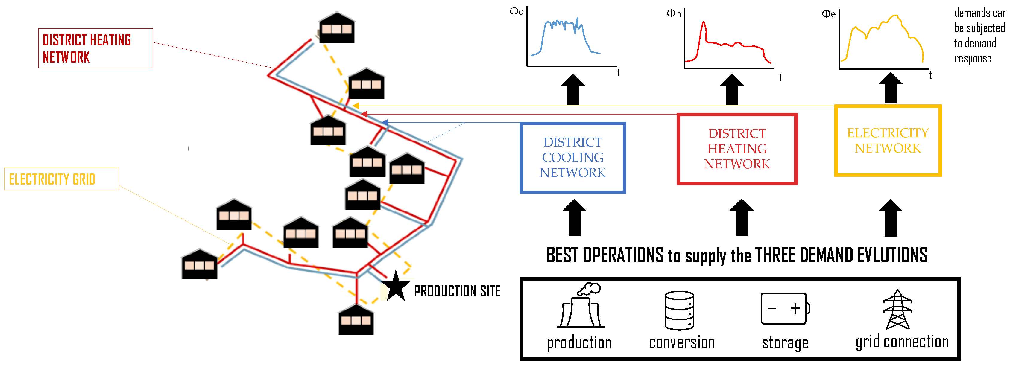
Multi-energy systems are typically characterized by the availability of various technologies, which can be combined in different ways to cover the demand for electricity, heating, cooling, etc. The main design parameters are the kind and the sizes of the technologies installed, their connections, and the characteristics of the energy infrastructure. The various combinations can provide different outcomes in terms of total energy cost, primary energy consumed, emission, etc. Among the various combinations, it is possible to find an optimal solution depending on the goal expressed by the objective function (e.g., minimum cost, carbon emission, primary energy). The best operation continuously changes in time since this depends on the various demands (electricity, heat, and cold), the ambient conditions, the constraints on the available technologies, etc. The optimization becomes much more complicated in case the system is connected to a district heating or/and one or multiple thermal energy storages. In these cases, the analysis is time-dependent. This means that the mathematical optimization cannot be solved separately for each time step, but this requires the solution to be obtained over a representative period (hours or days). This makes the number of independent variables much larger, as the set of variables is repeated within each time step. Various models have been proposed in the literature to face this kind of problem [6]. Linear programming is used when the technology efficiencies do not vary with the thermal load [7]. Most of the studies have been performed using mixed integer linear programming, both operation [8,9] and design [10] optimization. Non-linear programming or mixed integer non-linear programming is usually reserved for problems that are highly non-linear [11]. Results of the literature analysis show that the optimization of energy systems guarantees cost savings of the order of 5–25% [12,13] and CO2 emission reductions of 5–9% [14,15]. A graphical representation of the problem is provided in Figure 1.
1.3. Thermal Demand Response for Improving MED Operations
Consumers represent a major element of any smart energy system [16]. A very interesting approach to reducing the operating cost consists in modifying the plant load evolution in order to better fit optimal production. This result can be obtained through the application of demand response techniques, i.e., proper modifications of the building energy demand [17,18], which are still acceptable by the end-users. Demand response in multi-energy districts can provide significant results when applied to thermal networks [19] as thermal demand response has intended the possibility of relying on the thermal mass of buildings to modify the thermal demand profile of a building without significantly affecting the comfort conditions of the end-users (for more details, refer to the review paper [20]). Such an approach can be implemented by acting on the thermal schedule (i.e., the times the thermal substations of the buildings connected with the district heating network are switched on and off) as well as the specific climatic settings on the building side. Several works in the literature report the advantages associated with thermal demand response: (1) thermal peak shaving, which allows one avoiding the use of less efficient technologies as show in the experimental works, where peak cut of 25–30% [21] and 15% [22] are obtained; (2) more constant daily demand; in [23] the load factor is shown to increase from 0.2 to 0.44; (3) primary energy savings (a 4% reduction is reported in [24]) and reduction of the energy cost (3–5% in [25], 9% in [22]).
The adoption of thermal demand response in the optimization of a multi-energy system provides additional benefits in terms of cost reduction due to the possibility of combining load variations with the use of the most advantageous technologies depending on the availability of resources and the efficiency of each plant. In the literature, only a few works addressing the optimization of the multi-energy district by means of thermal demand response can be found. These works are mainly focused on the search for the optimal operation of the available energy conversion systems, often combined with thermal storage. The combination of supply-side optimization with demand response in the multi-energy district is addressed in a few studies, such as [25,26]. In [27], a technique for the optimization of the multi-energy district subject to demand response is proposed, also taking into account the thermal network dynamics. In works such as [28,29], it is shown that thermal network dynamics are usually neglected. Thermal network dynamics is the factor that makes the thermal loads at the plants different (in some cases to a large extent) from the summation of the thermal demand at the buildings due to the presence of the following:
- (a)
- different time delay of the water streams exiting the various buildings to reach the plant, depending on the building distance to the plant and their schedule;
- (b)
- thermal losses in pipelines during both operation and non-operation hours;
- (c)
- the thermal inertia due to a large amount of water inside.
Therefore, the difference between the load (at the plant) and the demand (at the buildings) is due to the network thermal dynamic impact, along with factors related to the substation/heating circuit. Especially in the case of large networks and discontinuous operations, it is actually important to consider this factor. When considering the network dynamic simulation, the computational cost significantly increases. An interesting approach is proposed in networks [28], where the computational costs start from 30 min, in the case of small-scale networks.
1.4. Work Contribution and Research Gaps
In this work, the authors present a methodology for the fast optimization of multi-energy districts where thermal demand response is applied; the contribution of the thermal network dynamics is performed by means of a simplified approach which allows one to obtain dramatic reductions in the computational time, without large penalties on the optimization results. The developed methodology relies on the solution of a programming optimization, estimating the best set of technologies for each time step, considering their proper efficiencies and costs and the influence of the storage availability.
The main strengths and novelties of the work are:
- (1)
- district heating simulation is included in the multi-energy district optimization along with demand response, which is conducted just in a few other works in the literature. Except for very few works, thermal demand response is applied to a predefined set of the operational condition of the production side (i.e., once the production is available, demand response activities with the aim of minimizing costs). In this new perspective, demand response is included in the plant operational management;
- (2)
- a specific approach is developed to reduce the computational costs to make it suitable for real-time network management and for the analysis of multiple realistic scenarios (e.g., in stochastic optimization), also in the case of large networks;
- (3)
- a realistic case study in terms of the number and type of generators, energy demand profiles, energy prices, storage size, is considered.
Results show that the adoption of the optimized strategy with demand response for the management of the technologies and the thermal storage allows a cost reduction of about 3% and that the efficacy of the fast optimizer is close to the full optimizer (−3% vs. −3.6%). Computational time dramatically reduces from 2700 s to 1 s.
1.5. Paper Structure
The paper structure is reported here. The optimization approach used to simulate a multi-energy district with demand response is described in Section 2.1 (specifically, the part related to demand response is described in Section 2.1.2). The Thermo-fluid dynamic model of the network is described in Section 2.2. The innovative approach proposed in this work and the reason for the choices done are described in Section 2.3. In Section 3 the case study is presented; information on the energy system considered (Section 3.1) and specific details on the demand response approach adopted (Section 3.2) are reported. The results are discussed in Section 4, in terms of production patterns (Section 4.1), operating costs (Section 4.2), and computational costs (Section 4.3). A discussion section is added (Section 5) to discuss the extension of the results to other cases, the model strength/limitation, and the applicability of the model proposed in relation to other available approaches. Conclusions are reported in Section 6.
2. Methodology
2.1. Problem Definition
2.1.1. Best Operations
The best operation for the energy system, i.e., the one that minimizes the cost of the energy supplied, is obtained by applying an optimization. The objective function is the total cost of the energy systems (Equation (1)), namely the sum of the operating energy costs of the various energy vectors purchased by the system minus the cost of the energy vector sold to the extern:
Costs are computed by multiplying the specific costs of gas and electricity times the corresponding energy flows. The specific costs are, for each time step, known; the quantities of energy purchased/sold are a consequence of the operating conditions. Therefore, power fluxes (electrical, heat, and cold) produced by each technology installed or stored/released by the thermal/electricity storages are the independent variables of the optimization. In the cases considered in this work, the conversion/storage technologies are five: gas Combined heat and production (CHP) units, gas heat only boiler (HOB), electric heat pump (EHP), and cold and thermal storage (see Section 3). All the time steps must be optimized in a unique optimization since the hot and cold storage operations make the problem time-dependent (i.e., the load at a certain time, t1, is dependent on the load at whatever other time, t2). The overall number of variables is thus the product of the number of technologies () times the time step considered in the analysis (here 96). This constitutes group A of independent variables; the remaining part, group B, is related to the application of the demand response.
Considering, therefore, the presence of various technologies absorbing and producing/releasing energy in the system, the total cost can be written as Equation (2), where the cost for each timestep and each technology can be estimated as in Equation (3).
where P is the power absorbed/released by each technology and c is the cost of the energy vector in input for each technology. In case of excess production, the specific cost is the sale cost of the energy vector times the amount of energy sold. The relation among sources and products of the technologies (therefore between chemical/thermal/electrical energy vectors) is a function of their efficiency. When the efficiency of the production and conversion technologies is independent of the load, the correlation between the source and product is linear. Otherwise, the results are non-linear. In this application, efficiencies are considered constant, according to the data reported in Table 1. Another important factor is, especially for heat pumps, the dependency of efficiency on the production temperature; in this case, since the water supply temperature is constant, the dependency has not been considered. However, the approach proposed is also valid for the non-linear problem, as clarified in Section 2.3.
The constraints of the optimization concern:
- The energy balances. The produced/purchased electricity, hot and cold energy, must be, at each time step, sufficient to supply the loads. The equation, for each energy vector v, and each time step j, has the form of Equation (4):where nPrTech_v, nStOut_v, nStIn_v, and nConvTech_v are, respectively, the technologies producing v, the storages releasing v, the storages are absorbing v and the conversion technologies absorbing v. and are the fluxes of the vector v that are respectively purchased and sold by the multi-energy district. Equation (4) is applied to the thermal, the electricity, and the cooling load, for each time step j.
In the case of thermal load (right-hand-side term), the production is performed with combined heat and power plant and heat only boiler (1st left-hand-side term), thermal storage is available (2nd and 3rd right-hand-side term), there are no technologies absorbing heat (4th right-hand-side term) and no other ways exist for purchasing/selling heat (5th and 6th right-hand-side term).
In the case of cooling load (right-hand-side term), the production is performed with an electric heat pump (1st left-hand-side term), and no other technologies exist that: act as cooling storage (2nd and 3rd right-hand-side term), absorb cooling (4th right-hand-side term) allows purchasing/selling cold (5th and 6th right-hand-side term).
In the case of electricity load (right-hand-side term), the production is performed with CHP (1st left-hand-side term), there is battery storage (2nd and 3rd right-hand-side term), there is the electric heat pump absorbing electricity (4th right-hand-side term), and it is possible to purchase/sell electricity from/to the grid (5th and 6th right-hand-side term).
- b.
- The efficiency of the technologies. As discussed before in this section, the efficiency (and COP in the case of heat pumps) of each technology is constant. Therefore, the following expression can be considered for the ith technology:where and are the flux of vector v, exiting and entering the technology.
- c.
- The storage capacity. The energy storages have a limited capacity, which is considered by means of constraints in the form of Equation (6):where, considering storage of the energy vector v, is the energy stored at t = t0, is the storage capacity, and are respectively the energy flux stored and released in the time step Δt.
2.1.2. Demand Response
As concerns the application of demand response, this is applied in the form of demand shifting (e.g., modification of the switching on/off time). Often, demand shifting can be applied using a discrete time step. Therefore, a fixed shifting of the demand must be planned. As largely discussed in Section 3.2, only discrete (every 5 min) anticipations up to 30 min are considered in this work, while no delays are considered. The anticipation represents the optimization variables related to the demand response (group B). The independent variable vector of group B has as many elements as the number of buildings subject to DR. The nature of the discrete variable is an integer.
2.2. Thermo-Fluid Dynamic Contribution
A thermo-fluid dynamic model of the network is applied to take into account the contribution of the following phenomena occurring in the pipeline:
- -
- mixing between streams at different temperatures;
- -
- thermal losses;
- -
- thermal transients.
A one-dimensional thermo-fluid dynamic model is used in this study. Graph theory was used to describe the structure of the network; each pipe is viewed as a branch, delimited by two nodes which are the inlet and outlet cross sections and coincide with junctions between two/more pipes or between the pipe and the boundary of the system. The incidence matrix, A, describes the network topology. The incidence matrix Aij has the same number of rows as the number of network nodes (NN) and the same number of columns as branches (NB). The matrix elements are equal to 1 if the i-th node is the inlet node of the j-th branch, 1 if it is the outlet node, and 0 if the i-th node and the j-th branch are both nodes. The model is based on the conservation equations: mass, momentum, and energy, shown in Equations (7)–(9). The model is adopted in pseudo-dynamic. This means that the hydraulic problem, composed of Equations (7) and (8), is considered in steady-state conditions at each time step while the energy equation, Equation (9), is solved dynamically. This is because temperature perturbations travel at the fluid velocity and may take a long time to propagate within the network, while the fluid-dynamic perturbations (pressure waves) are very rapid, traveling the entire network in a few seconds. In the energy equation, the conductive term is neglected, and the network capacity term is considered [30].
where p, G, and T are, respectively, mass flow rates, pressures, and temperatures in the system. D, L, and S are, respectively, the diameter, the length, and the section of the pipes. f and β are the distributed and concentrated friction factors. Variables , c, and U are, respectively, density, specific heat, and global heat transfer coefficient. The problem solution is conducted numerically using a finite volume approach [31].
Since mass-flow rates in a three-shaped network are independent of the pressure distribution within the network, they may be calculated with ease from the solution of Equation (5). Equation (6) is therefore neglected in this analysis. The matrix form of mass and energy conservation equations are reported respectively in Equations (10) and (11):
where vectors G and T are the unknowns of the problem, containing the mass flow rates and the temperature, respectively, in each branch and node of the system. A is the incidence matrix, is a vector including the amount of mass flow that is inserted and supplied in the boundaries of the system (i.e., at the thermal plants and at the customers). The stiffness matrix K and the mass matrix M include, respectively, the coefficient multiplying the temperature and its derivative; g includes the known terms of the equation. Further details on the model adopted can be found in [32]. The boundary conditions for the problem are, respectively, the mass flow rates required by each building for the mass conservation equation and the temperature of the mass flow rates entering the system for the energy conservation equation. As a concern for the initial condition, the steady state solution of the problem at t = t0 is adopted.
2.3. Problem Solution
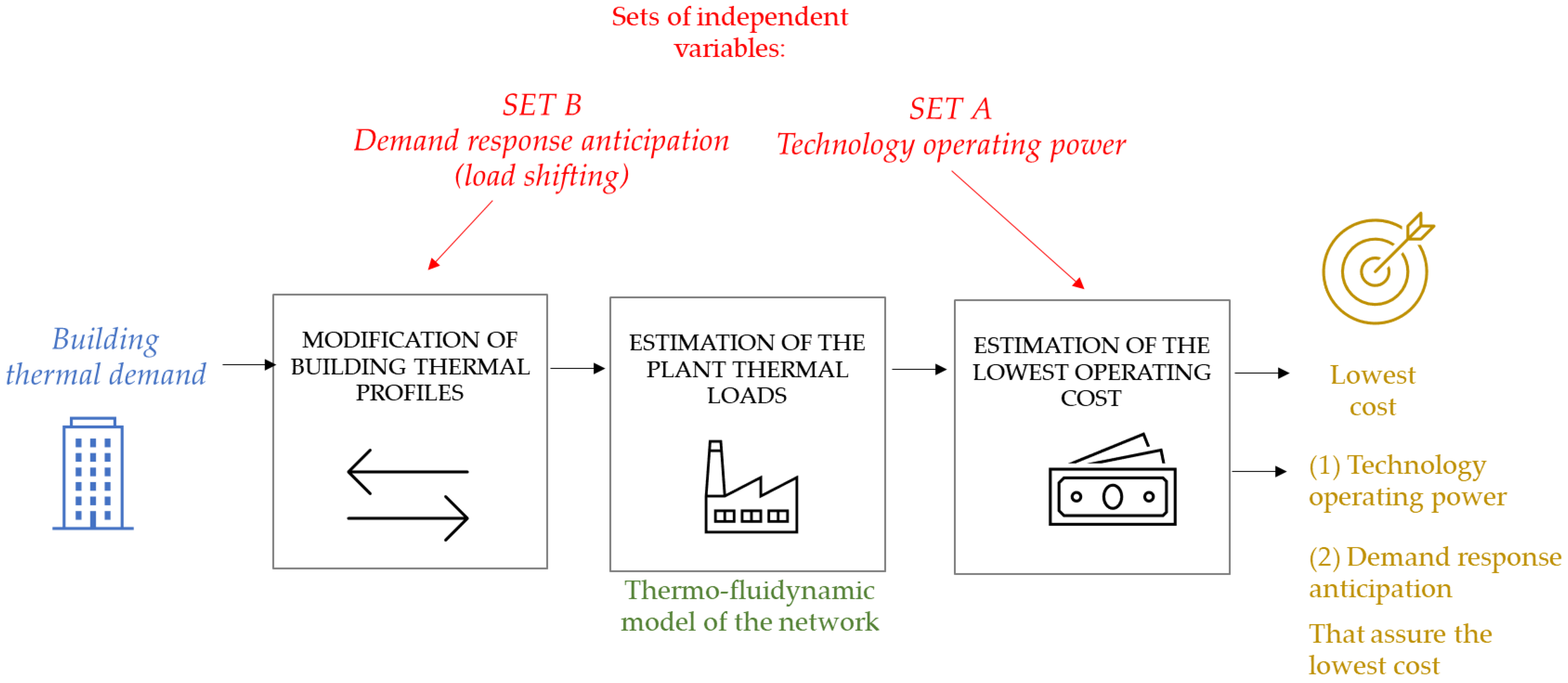
The problem defined in Section 2.1 considers the thermo-fluid dynamics of the network to obtain the plant loads, given the building demands. The independent optimization variables are the thermal power of the different technologies (group A) and the demand response anticipations (group B). Therefore, a general problem solution has the following structure, as schematized in Figure 2):
- Definition of building thermal profiles (input of the problem).
- Modification of the building thermal profiles according to the set of independent variables of the demand response (group B).
- Adoption of the thermo-fluid dynamic model of the network for the estimation of the plant loads, given the building thermal profiles.
- Use of the plant thermal load for the estimation of the cost using the independent variable of group A.
In a generic optimization process, the groups A and B of the independent variables are the outcomes of the optimization. The problem defined is a mixed integer for the presence of the variable related to demand response (integer, since the variations admitted, are discrete) and in case of non-linear efficiency of the conversion technologies. The presence of the thermo-fluid dynamic model of the network makes the problem not suitable for classic MILP solvers. For this reason, other approaches have been adopted in the literature, as shown in [19]. The model proposed by the author, called fast optimizer, is used as a reference for comparison with the new approach (called full optimizer).
Figure 2.
Schematic of the general logic for the solution of demand response-multi-energy system problems.
Figure 2.
Schematic of the general logic for the solution of demand response-multi-energy system problems.

2.4. Fast Approach Proposed
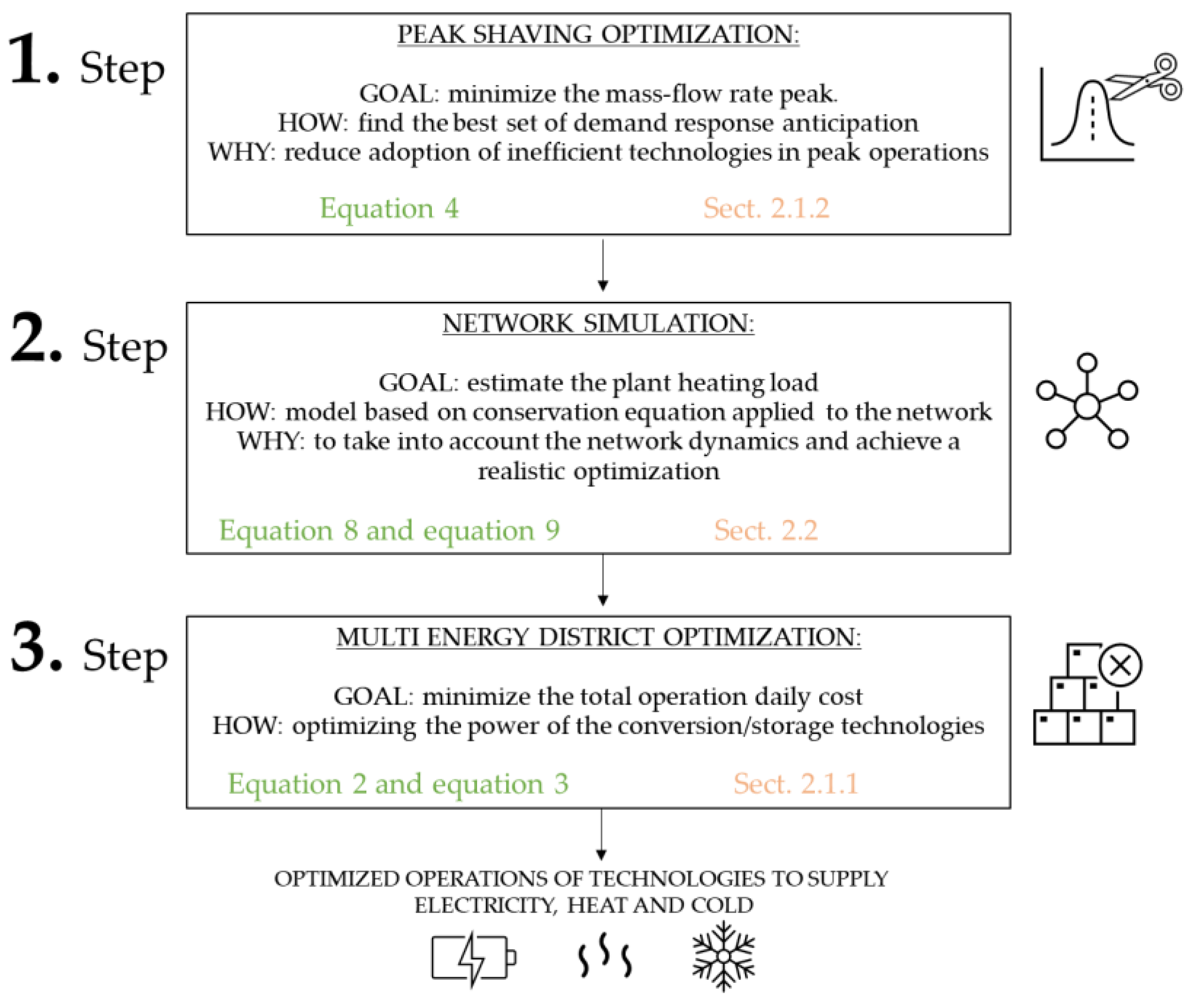
In this work, a novel approach is proposed for fast simulation. This is composed of different steps, as schematized in Figure 3:
- Hydraulic optimization. The first step consists of the selection of a set of optimal load shifting, which minimizes the peak mass-flow rate. This allows to minimization of the mass-flow peak required by the users. The first step allows thus to estimate the heating demand anticipation of each building such that
The optimization is solved with a mixed integer linear programming using the solver Gurobi.
- Plant heating load estimation. The second step consists of the estimation of the plant heating load given the building thermal demand, which is a consequence of the best set of anticipations (output of step 1). The estimation of the plant thermal load is conducted through physical simulation of the district heating network. This is performed to take into account mixing, delays, and thermal transients, occurring within the pipelines. The thermo-fluid dynamic model of the district heating network is described in Section 2.2.
- Multi-energy district optimization. In the last step, the optimization of the operation of the multi-energy system, given the thermal demand estimated in step 2, is done. The aim is to find the best set of thermal power for each production/conversion/storage technology (P in Equation (3)) with the aim of minimization of the daily operating cost (Equation (1)). The problem solution is conducted with a Mixed Integer Linear Programming (MILP) approach. This means that the approach is also suitable in the case of non-linear efficiencies since these can be easily piecewise linearized. The details of the optimization problem are given in Section 2.1.
This approach is conceived with the aim of separately estimating the best set of thermal power for the multi-energy district and the best demand response to apply to the buildings. This allows for significantly reducing the computational time required for the solution of the problem, as shown in the Result section.
Here the idea behind the model just presented is discussed. The peak creation is a consequence of two aspects. The first is related to the temperature drop in the network during thermal transient, which occurs when a part of the system is not operating (e.g., during the night). In this case, the mass flow is zero or very low. The water cools down quite rapidly because of the larger thermal losses. During the system switching on, the demand is much higher to recover the normal operating temperature of the water. This has an impact on peak creation. The second is related to the larger mass flow rate. The substation valve, after the switching off/attenuation, opens completely to ensure a reheating of the secondary circuit/substation heat exchanger/heating devices, making dramatically increasing the mass flow rate within the pipelines [33]. The impact of the first contribution is mainly dependent on the quantity of water within the network and, therefore, on the network dimension and on the number of temperature fluctuations. In the case of small networks or small temperature fluctuations, the contribution of the first factor is not significant as the contribution due to the mass flow increase. This is proved by previous results of an author published in [29]: if in large networks, the dynamic of the system should be considered, in small networks, or networks with no large thermal transients, this can be neglected. The approach presented here is focused on networks where this contribution is not large.
The idea is that in these cases, it is possible to decouple the simulation of the thermal transient from the optimization of demand response without losing most of the optimization result accuracy. The best demand response anticipations are therefore estimated, considering only the second contribution to the peak shaving due to the mass flow rate increase; for this reason, the mass flow rate is minimized.
Figure 3.
Schematics of the approach adopted for fast simulations.

3. Case Study
3.1. District Heating Details
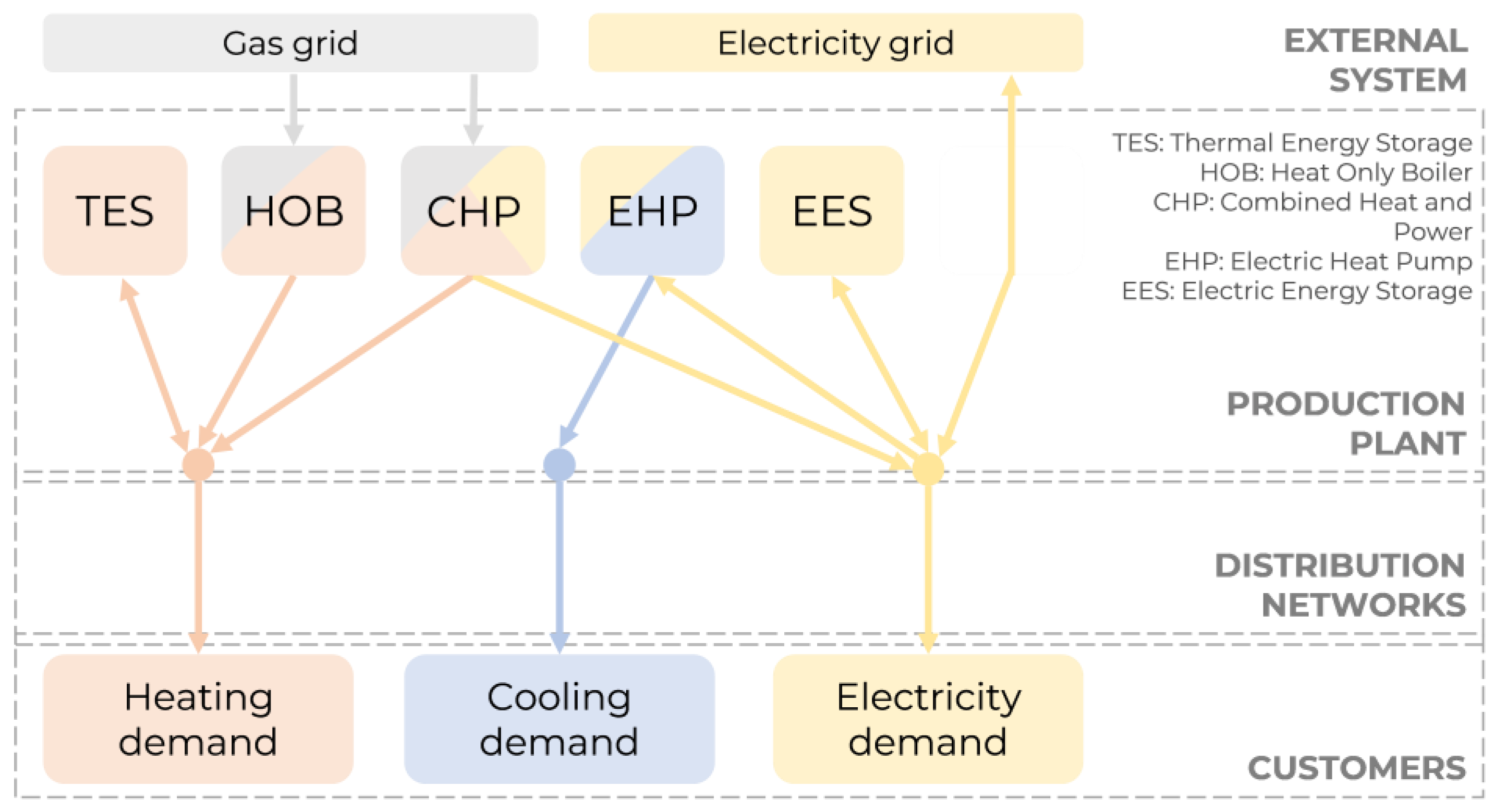
In the present work, a small network is considered a case study since the method is specifically conceived for a system with moderate thermal transients, as detailed in Section 2.3. This includes industrial, office, and residential users. The total number of connected substations is 60. The district heating network is characterized by 202 nodes and 201 branches for a total length of 4.5 km. The multi-energy system is characterized by a set of technologies for the production/conversion and storage of energy.
- Heat production: heat can be supplied with a combined heat and power (CHP) unit and with a natural gas boiler (HOB).
- Electricity Production: electricity can be produced using the CHP and by grid purchase.
- Cooling production: cooling is produced using the Electric heat pump.
Furthermore, electrical storage and thermal storage are considered. Details on the installed technologies are provided in Table 1. A schematic of the connection of the conversion and storage units is provided in Figure 4. As concern the costs, the electricity costs range from 0.02 and 0.08 €/kWh for selling and from 0.15 to 0.2 €/kWh for electricity purchase. Gas cost is 0.021 €/kWh.
3.2. Thermal Demand Response
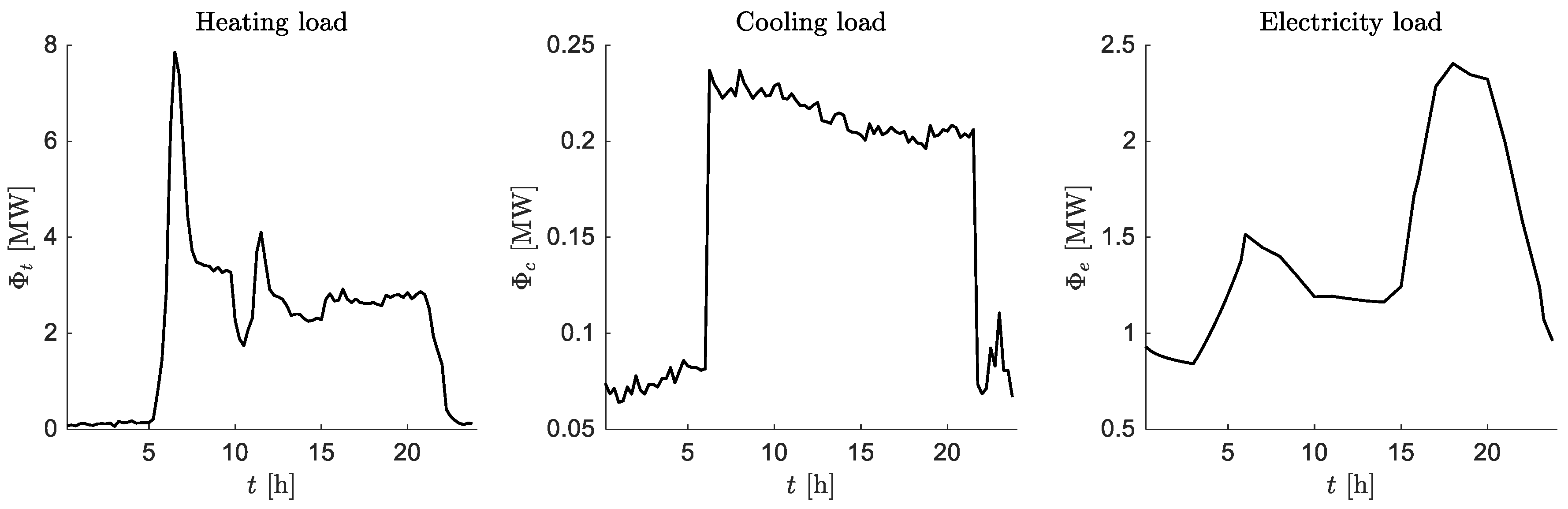
The analysis is conducted on a typical mild winter day. The heating, cooling, and electricity loads are reported in Figure 2. Concerning the electricity demand, this never goes to zero. A certain demand is always present, and in particular, this is higher in the evening. The cooling load is much lower than the other loads since this is only required for industrial applications.
As concern the heating load, this has a significant thermal peak in the early morning. In areas with milder winters, such as the Mediterranean, the building occupants often have the habit of shutting down or remarkably attenuating the heating devices at night. This habit creates, as a consequence, a typical thermal demand profile, as the one reported in Figure 5. In the morning, the systems are switched on, and a significant thermal peak occurs because of the two main reasons largely discussed in Section 2.3. Peaks are usually supplied with low-efficiency plants; therefore, it is worth shaving them. This is mainly conducted by using demand response or thermal storage. Storages allow for flexible management but, on the other hand, require space and investment. In the present analysis, thermal storage demand side, management is adopted as a further technique to shave the peak and increase the overall efficiency.
With thermal demand response, the thermal demand of the users can be changed in the optimization tool according to the requirements of the system. In the present case study, demand shifting is considered, which allows the achievement of significant peak reduction without modifications in the system control strategy [34,35]. In order to prevent affecting the users’ thermal comfort, only anticipations up to 30 min are allowed. No delays are considered to avoid unsatisfactory comfort conditions in the morning. In case anticipation is larger than 30 min, suitable tools for the simulation of the indoor conditions or direct smart sensors for measuring temperatures should be used to maintain satisfactory internal comfort. The demand shifting, as often happens in a real network, can be applied only on a discrete basis, every 5 min, due to reasons related to the controller adopted. Therefore, the possibilities for demand response are 5, 10, 15, 20, 25, and 30 min.
4. Results
4.1. Load Profiles
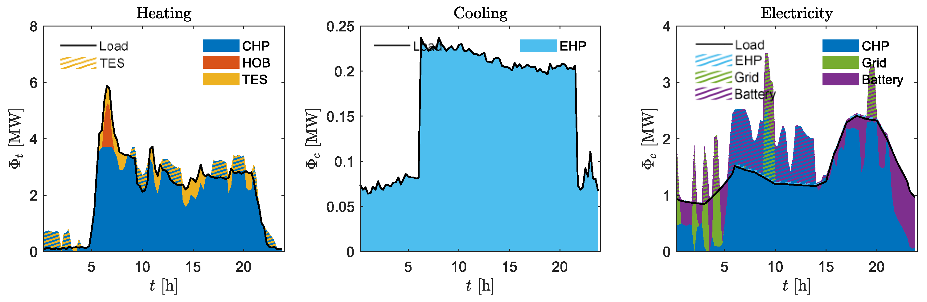
In this section, the optimal operation of the multi-energy district technologies that allow supplying of the three total load profiles at the minimum overall cost is reported. Figure 6 shows the results of the optimization performed with the fast approach proposed. In black, the load evolutions are reported. The black curve is filled in different colors, depending on the technology adopted to supply the energy. In striped colors, the energy that is produced in excess is reported. The excess energy is used (a) to be sold (e.g., electricity sold to the grid), (b) to be stored (e.g., thermal energy in the thermal storage), (c) to supply other conversion technologies (e.g., electricity must be produced in excess to supply the EHP). Cooling is entirely produced by using the EHP, which is the only available technology. The heating base load is produced using the CHP. The HOB is used to supply the morning peak, along with thermal storage. Concerning the electricity, the base load is produced by CHP. Electricity is stored when the load is lower to the CHP production and released for valley filling.
Results obtained with the fast approach are compared with the results achieved with the conventional approach [19]. The same comments made for the fast optimization results apply to these results. Only small differences are present between the evolutions of Figure 6 and Figure 7, mainly due to slightly different management of the storage. The same technologies are adopted to supply the multi-energy district, which has very similar load evolutions.
4.2. Total Cost
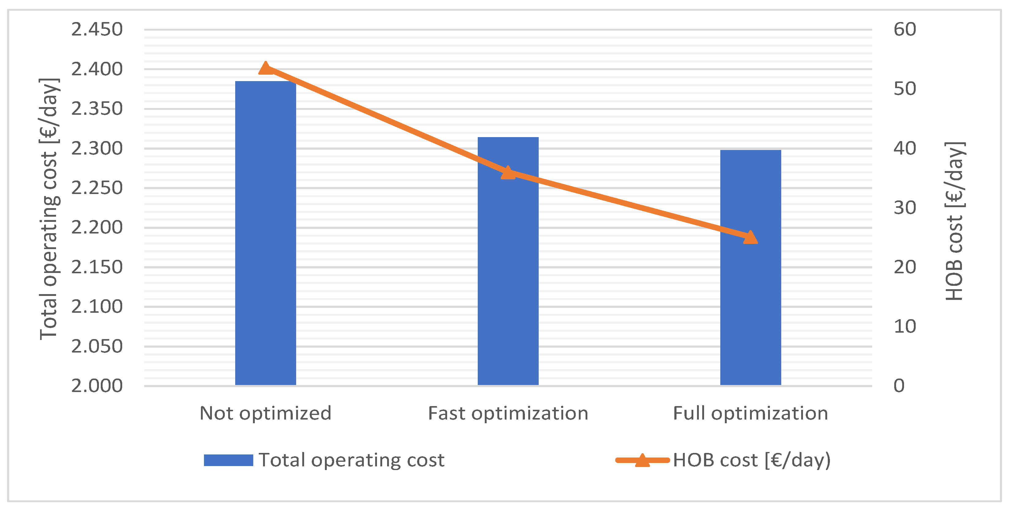
Figure 8 presents a comparison of the total costs obtained with the two optimizations depicted in Figure 6 and Figure 7. The comparison also includes the case of operation optimization with demand response. Therefore, the three bars and the line represents respectively, are the overall daily operating costs and the daily cost related to the boiler technology in three cases: (a) optimization without demand response, (b) fast optimization with demand response, (c) with the full optimization with demand response. At first, it is possible to state that the adoption of demand response allows for a significant reduction of the operating cost. The cost without demand response is 2385 €/day, while the minimum cost of the fast and full otimizer are respectively 2314 €/day and 2298 €/day. This means that a reduction of 3% and 3.6% is achieved in the two cases. Both these differences are significant for the operation of an energy system. The difference in the total cost obtained using the fast optimization (2314 €/day) and the full otimizer (2298 €/day) is 16 €/day. The difference is not negligible but limited. In particular, it should be considered that in several cases, the uncertainty related to the thermal demand could make this difference smaller or even inverted; in these cases, the fast approach could represent a favorable option since it can be adopted and included in stochastic optimization. On the other hand, the cost reduction related to the use of heat-only boiler is significant between the fast and full optimization approach (36 €/day for the fast vs 25 €/day for the full). The difference is that the thermal transients have been neglected. This result suggests that, in large networks characterized by significant thermal transient, this could provide large cost increases. Nevertheless, the large computational time required by the full approach might force one to accept a sub-optimal result obtained with the fast approach (see next section).
4.3. Computational Resources
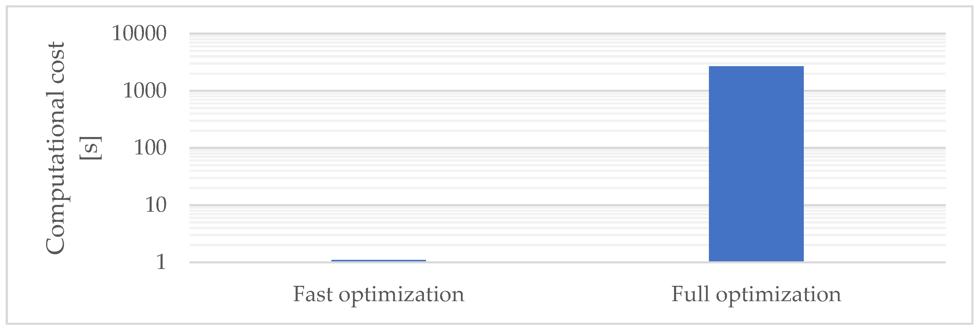
The computational costs for running the fast and the full optimizations are completely different. These are shown in Figure 9 for a PC laptop with a total of 16 GB of memory and an Intel i7-8565U CPU @ 1.80 GHz. The fast optimization only takes 1 sec to provide results. The full optimization approach requires about 45 min. This is not an unsustainable time, in general. It depends on the application. For obtaining a one-day ahead optimization, i.e., to plan the daily operation for the following day, this is a reasonable time. For having a real-time optimization, with the aim of updating the results of the previous simulation, given updated profile data, this is not suitable. In this case, fast optimization is preferable. The same applies in the case of multi-scenario simulation (e.g., for stochastic analysis). These aspects are discussed in Section 4.
5. Discussion
The idea of the approach developed in this work was born while observing (a) the high computational costs required to solve multi-energy district operation optimization with thermal demand response and (b) the different impacts of the thermal transient in different kinds of networks/loads. The authors decided to develop and test a fast approach, specifically for cases characterized by (a) a small network (i.e., with small pipe lengths and diameters) and (b) thermal loads that do not cause significant temperature variations within the network.
Comparison with/without demand response: The comparison shows that the demand response provides non-negligible overall cost savings. The saving range between 3 to 3.6%. As concern the extension of the result on another multi-energy district, the saving is expected to strongly depend on various aspects. The first is the entity of the peaks. The second is related to the technologies adopted to supply the network; when technologies with completely different efficiency are available, the saving due to proper peak management significantly increases. The third is the thermal storage availability; when the storage capacity is large, the benefits related to demand response reduce. In the present case study, there is a large thermal peak, and the efficiency of thermal production technologies (CHP and HOB) are very different. Therefore, the thermal storage is designed with a large size. In such a case, the application of demand response to the multi-energy district offers limited advantages with respect to a case in which the storage is small. Although the obtained reduction in the total costs (3.6%) is a good result, it is not an upper limit for the combined optimization of demand response and multi-energy systems operation. Reductions over 5% can be easily achieved when the size of thermal storage is optimized, considering the possibility of combining it with the application of demand response techniques.
Comparison fast/full optimization. A comparison of results for the present case study shows that the full model guarantees moderately higher performance (+0.6% saving) with a time requirement considerably higher (+99.9% of the time). Therefore, it is important to correctly select the approach, depending on the application.
The full optimizer, as already reported in Section 4.3, can be used for:
- one-day ahead optimization: this is useful for planning the daily operation of the following day.
- analyses for further development: the model can be extremely useful to simulate future benefits achievable by installing new technologies, adopting different demand response techniques, applying innovative control strategies, or changing the thermal network operating conditions.
- design purposes: the model can be adopted to design a multi-energy district, taking into account the future operation, which allows more focused planning.
The fast optimizer is suitable for different applications:
- real time optimization: this is useful to achieve fast indications for the current system operation. This can be very useful also in combination with a one-day ahead optimizer, with the aim of updating the results of the day ahead simulation, given the updated building demand profiles of the current day.
- multi-scenario simulation: there are cases in which the uncertainties on the building thermal demand or the characteristics of the devices/network are significant. In these cases, a multi-scenario or a stochastic optimization can be useful to minimize the impact of uncertainties and unknowns on the results. Fast models are required to keep reasonable the computational time of the simulation.
- Large scale network with moderate thermal transient: this refers to the case of large networks when the computational time required to run the full model would be unsustainable. In particular, when the thermal peak is mainly due to mass flow increase, and not this is not related to the transient temperature difference, this approach could be adopted.
When implementing the approach into reality, a demand forecast is mandatory. Therefore, in order to minimize the impact of demand uncertainty, a good precision demand forecast should be adopted. At the same time, morning peak prediction can reach a good level of accuracy since (a) the switching on time is known in advance and (b) the thermal peaks are less dependent on the environmental temperature than the demand at other times (e.g., during late morning or afternoon) since the night cooling down of the DH infrastructure (e.g., the pipelines) is more independent from the outdoor temperature than the building steady state load.
Another important point concerns the optimization purpose. In this case, the purpose is the operation optimization of an already existing system. In case the goal was the contemporary design and optimization of the system, the significant change required would be the addition of new integer variables, i.e., the investment cost of the technologies installed. The solution can therefore be performed with the same cascade MILP approach proposed in the current work.
Future research directions should include the analysis of multi-energy districts that include large-scale district heating. This is a challenging topic because of two reasons. First, in a large network characterized by significant load variations, the thermal inertia, if neglected, could significantly impact the results. Secondly, large thermal networks are characterized by complex topologies and a large number of pipes; this significantly increases the number of variables of the optimization problem.
6. Conclusions
This paper proposes a fast approach to perform instantaneous optimization of multi-energy districts with thermal demand response. The approach decouples the demand response and the operation optimization, neglecting, in the demand response optimization, the impact of the thermal inertia. Between the two optimizations, the network model is applied to ensure to supply of the actual amount of heat required by the network. The approach is tailored for small-scale district heating system or medium/large if the temperature variations are limited since, in these cases, the contribution of the thermal inertia is low and the thermal transients in the network do not play a crucial role in the peak creation.
Results show that the adoption of optimization in operation is useful to reduce the operation costs of the multi-energy system by order of 3%. The fast optimizer provides satisfactory results as concerns the operating cost reduction: −3% vs. −3.6 of the full approach. At the same time, the computational time required is much lower (−99.9%).
In conclusion, the full approach presented here can be considered suitable for all the cases in which the computational cost must be low, such as real-time operations or multi-scenario. Future development will consist of the individuation of a possible approach to address the same problem in large-scale DH.
Author Contributions
Conceptualization, M.C. and E.G.; methodology, M.C.; investigation, M.C. writing—original draft preparation, M.C.; writing—review and editing, E.G.; supervision, E.G. All authors have read and agreed to the published version of the manuscript.
Funding
This research received no external funding.
Institutional Review Board Statement
Not applicable.
Informed Consent Statement
Not applicable.
Data Availability Statement
Not applicable.
Conflicts of Interest
The authors declare no conflict of interest.
References
- Pelda, J.; Stelter, F.; Holler, S. Potential of integrating industrial waste heat and solar thermal energy into district heating networks in Germany. Energy 2020, 203, 117812. [Google Scholar] [CrossRef]
- Guelpa, E.; Bischi, A.; Verda, V.; Chertkov, M.; Lund, H. Towards future infrastructures for sustainable multi-energy systems: A review. Energy 2019, 184, 2–21. [Google Scholar] [CrossRef]
- Clegg, S.; Mancarella, P. Integrated Electrical and Gas Network Flexibility Assessment in Low-Carbon Multi-Energy Systems. IEEE Trans. Sustain. Energy 2016, 7, 718–731. [Google Scholar] [CrossRef]
- Mancarella, P. MES (multi-energy systems): An overview of concepts and evaluation models. Energy 2014, 65, 1–17. [Google Scholar] [CrossRef]
- Werner, M.; Muschik, S.; Ehrenwirth, M.; Trinkl, C.; Schrag, T. Sector Coupling Potential of a District Heating Network by Consideration of Residual Load and CO2 Emissions. Energies 2022, 15, 6281. [Google Scholar] [CrossRef]
- Allegrini, J.; Orehounig, K.; Mavromatidis, G.; Ruesch, F.; Dorer, V.; Evins, R. A review of modelling approaches and tools for the simulation of district-scale energy systems. Renew. Sustain. Energy Rev. 2015, 52, 1391–1404. [Google Scholar] [CrossRef]
- Ren, H.; Zhou, W.; Nakagami, K.; Gao, W.; Wu, Q. Multi-objective optimization for the operation of distributed energy systems considering economic and environmental aspects. Appl. Energy 2010, 87, 3642–3651. [Google Scholar] [CrossRef]
- Bischi, A.; Taccari, L.; Martelli, E.; Amaldi, E.; Manzolini, G.; Silva, P.; Campanari, S.; Macchi, E. A detailed MILP optimization model for combined cooling, heat and power system operation planning. Energy 2014, 74, 12–26. [Google Scholar] [CrossRef]
- Bischi, A.; Taccari, L.; Martelli, E.; Amaldi, E.; Manzolini, G.; Silva, P.; Campanari, S.; Macchi, E. A rolling-horizon optimization algorithm for the long term operational scheduling of cogeneration systems. Energy 2019, 184, 73–90. [Google Scholar] [CrossRef]
- Buoro, D.; Casisi, M.; De Nardi, A.; Pinamonti, P.; Reini, M. Multicriteria optimization of a distributed energy supply system for an industrial area. Energy 2013, 58, 128–137. [Google Scholar] [CrossRef]
- Arcuri, P.; Beraldi, P.; Florio, G.; Fragiacomo, P. Optimal design of a small size trigeneration plant in civil users: A MINLP (Mixed Integer Non Linear Programming Model). Energy 2015, 80, 628–641. [Google Scholar] [CrossRef]
- Mitra, S.; Sun, L.; Grossmann, I.E. Optimal scheduling of industrial combined heat and power plants under time-sensitive electricity prices. Energy 2013, 54, 194–211. [Google Scholar] [CrossRef] [Green Version]
- Yang, Y.; Zhang, S.; Xiao, Y. Optimal design of distributed energy resource systems coupled withenergy distribution networks. Energy 2015, 85, 433–448. [Google Scholar] [CrossRef]
- Ren, H.; Gao, W. A MILP model for integrated plan and evaluation of distributed energy systems. Appl. Energy 2010, 87, 1001–1014. [Google Scholar] [CrossRef]
- Marquant, J.F.; Evins, R.; Bollinger, L.A.; Carmeliet, J. A holarchic approach for multi-scale distributed energy system optimisation. Appl. Energy 2017, 208, 935–953. [Google Scholar] [CrossRef] [Green Version]
- Schweiger, G.; Eckerstorfer, L.V.; Hafner, I.; Fleischhacker, A.; Radl, J.; Glock, B.; Wastian, M.; Rößler, M.; Lettner, G.; Popper, N.; et al. Active consumer participation in smart energy systems. Energy Build. 2020, 227, 110359. [Google Scholar] [CrossRef]
- Gelazanskas, L.; Gamage, K.A.A. Demand side management in smart grid: A review and proposals for future direction. Sustain. Cities Soc. 2014, 11, 22–30. [Google Scholar] [CrossRef]
- Siano, P. Demand response and smart grids—A survey. Renew. Sustain. Energy Rev. 2014, 30, 461–478. [Google Scholar] [CrossRef]
- Capone, M.; Guelpa, E.; Mancò, G.; Verda, V. Integration of storage and thermal demand response to unlock flexibility in district multi-energy systems. Energy 2021, 237, 121601. [Google Scholar] [CrossRef]
- Guelpa, E.; Verda, V. Demand response and other demand side management techniques for district heating: A review. Energy 2021, 219, 119440. [Google Scholar] [CrossRef]
- Wu, Y.; Mäki, A.; Jokisalo, J.; Kosonen, R.; Kilpeläinen, S.; Salo, S.; Liu, H.; Li, B. Demand response of district heating using model predictive control to prevent the draught risk of cold window in an office building. J. Build. Eng. 2021, 33, 101855. [Google Scholar] [CrossRef]
- Ala-Kotila, P.; Vainio, T.; Heinonen, J. Demand response in district heating market—Results of the field tests in student apartment buildings. Smart Cities 2020, 3, 157–171. [Google Scholar] [CrossRef] [Green Version]
- Sweetnam, T.; Spataru, C.; Barrett, M.; Carter, E. Domestic demand-side response on district heating networks. Build. Res. Inf. 2019, 47, 330–343. [Google Scholar] [CrossRef] [Green Version]
- Wernstedt, F.; Davidsson, P.; Johansson, C. Demand Side Management in District Heating Systems. In Proceedings of the 6th International Joint Conference on Autonomous Agents and Multiagent Systems (AAMAS 2007), Honolulu, HI, USA, 14–18 May 2007. [Google Scholar]
- Hedegaard, R.E.; Kristensen, M.H.; Pedersen, T.H.; Brun, A.; Petersen, S. Bottom-up modelling methodology for urban-scale analysis of residential space heating demand response. Appl. Energy 2019, 242, 181–204. [Google Scholar] [CrossRef]
- Thang, V.V.; Ha, T.; Li, Q.; Zhang, Y. Stochastic optimization in multi-energy hub system operation considering solar energy resource and demand response. Int. J. Electr. Power Energy Syst. 2022, 141, 108132. [Google Scholar] [CrossRef]
- Reynolds, J.; Ahmad, M.W.; Rezgui, Y.; Hippolyte, J.L. Operational supply and demand optimisation of a multi-vector district energy system using artificial neural networks and a genetic algorithm. Appl. Energy 2019, 235, 699–713. [Google Scholar] [CrossRef]
- Capone, M.; Guelpa, E.; Verda, V. Multi-objective optimization of district energy systems with demand response. Energy 2021, 227, 120472. [Google Scholar] [CrossRef]
- Guelpa, E. Impact of network modelling in the analysis of district heating systems. Energy 2020, 213, 118393. [Google Scholar] [CrossRef]
- Capone, M.; Guelpa, E.; Verda, V. Accounting for pipeline thermal capacity in district heating simulations. Energy 2021, 219, 119663. [Google Scholar] [CrossRef]
- Versteeg, H.K.; Malalasekera, W. An Introduction to Computational Fluid Dynamics: The Finite Volume Method; Pearson Education Limited: London, UK, 2017. [Google Scholar]
- Guelpa, E.; Sciacovelli, A.; Verda, V. Thermo-fluid dynamic model of large district heating networks for the analysis of primary energy savings. Energy 2019, 184, 34–44. [Google Scholar] [CrossRef]
- Guelpa, E. Impact of thermal masses on the peak load in district heating systems. Energy 2021, 214, 118849. [Google Scholar] [CrossRef]
- Aoun, N.; Bavière, R.; Vallée, M.; Brun, A.; Sandou, G. Dynamic Simulation of Residential Buildings Supporting the Development of Flexible Control in District Heating Systems. In Proceedings of the 13th International Modelica Conference, Regensburg, Germany, 4–6 March 2019; Volume 157, pp. 129–138. [Google Scholar] [CrossRef] [Green Version]
- Aoun, N.; Aurousseau, A.; Sandou, G. Load shifting of space-heating demand in DHSs based on a building model identifiable at substation level Context Space-heating demand management. In Proceedings of the 4th Smart Energy Systems and 4th Generation District Heating Conference, Aalborg, Denmark, 13–14 November 2018. [Google Scholar]
Figure 1.
Schematic of the optimization of multi-energy districts.

Figure 4.
Schematic of the multi-energy considered in the analysis, with energy vectors and energy infrastructure (storage and conversion units).
Figure 4.
Schematic of the multi-energy considered in the analysis, with energy vectors and energy infrastructure (storage and conversion units).

Figure 5.
Load profiles.

Figure 6.
Fast optimization results: operations of the technology for the supply of heating, cooling, and electrical load.
Figure 6.
Fast optimization results: operations of the technology for the supply of heating, cooling, and electrical load.

Figure 7.
Full optimization results (Approach B): operations of the technologies for the supply of heating, cooling, and electrical load.
Figure 7.
Full optimization results (Approach B): operations of the technologies for the supply of heating, cooling, and electrical load.

Figure 8.
Comparison between total cost and HOB cost obtained without optimization, fast and full optimization.
Figure 8.
Comparison between total cost and HOB cost obtained without optimization, fast and full optimization.

Figure 9.
Comparison computational cost required for fast and full optimization.


Table 1.
Characteristics of the Technologies adopted in the multi-energy district.
| Technology | Acronym | Efficiency | Max Inlet Power (MW) | Energy Storable (MWh) |
|---|---|---|---|---|
| Natural gas combined heat and power plant | CHP | 0.36 | 7 | |
| 0.53 | ||||
| Natural gas heat only boiler | HOB | 0.92 | 6 | |
| Electric heat pump | EHP | 4.4 | 0.75 | |
| Thermal storage for heating purposes | Hot storage | 1 | 0.6 | 1.6 |
| Thermal storage for cooling purposes | Cold storage | 1 | 1 | 5 |
Disclaimer/Publisher’s Note: The statements, opinions and data contained in all publications are solely those of the individual author(s) and contributor(s) and not of MDPI and/or the editor(s). MDPI and/or the editor(s) disclaim responsibility for any injury to people or property resulting from any ideas, methods, instructions or products referred to in the content. |
© 2023 by the authors. Licensee MDPI, Basel, Switzerland. This article is an open access article distributed under the terms and conditions of the Creative Commons Attribution (CC BY) license (https://creativecommons.org/licenses/by/4.0/).
Share and Cite
MDPI and ACS Style
Capone, M.; Guelpa, E. Implementing Optimal Operation of Multi-Energy Districts with Thermal Demand Response. Designs 2023, 7, 11. https://doi.org/10.3390/designs7010011
AMA Style
Capone M, Guelpa E. Implementing Optimal Operation of Multi-Energy Districts with Thermal Demand Response. Designs. 2023; 7(1):11. https://doi.org/10.3390/designs7010011
Chicago/Turabian StyleCapone, Martina, and Elisa Guelpa. 2023. "Implementing Optimal Operation of Multi-Energy Districts with Thermal Demand Response" Designs 7, no. 1: 11. https://doi.org/10.3390/designs7010011