
CFD Investigation for Sonar Dome with Bulbous Bow Effect

Department of Systems and Naval Mechatronic Engineering, National Cheng Kung University, Tainan City 70101, Taiwan
*
Author to whom correspondence should be addressed.
Inventions 2023, 8(2), 58; https://doi.org/10.3390/inventions8020058
Submission received: 4 February 2023
/
Revised: 12 March 2023
/
Accepted: 17 March 2023
/
Published: 23 March 2023
(This article belongs to the Special Issue Recent Advances in Fluid Mechanics and Transport Phenomena)
Abstract
:The objective of this study is to design a hull-mounted sonar dome of a ship using OpenFOAM with a bulbous bow effect at cruise speed in calm water. Verification and validation for the original sonar dome simulation are conducted. Next, the 1.44 million grid size is selected to study different dome lengths. By protruding the dome forward 7.5% of the ship’s length, the optimal 17% resistance reduction is achieved and is mainly caused by the pressure resistance decrease. The optimal sonar dome not only functions in the same way as a bulbous bow, but the viscous flow behaviors are also improved. The protrusion corresponding to 90 deg phase lag reduces the bow wave amplitude. The flow acceleration outside the boundary layer and ship wake velocity are higher coinciding with the much lower total resistance. A smaller flow separation and thinner boundary layer are also observed behind the sonar dome because its back slope is less steep. The high pressure covers a smaller area around the bow, and the smaller bow wave crest does not hit the ship’s flare to form high pressure. Consequently, the lower high pressure on the dome front and higher low pressure on the dome back result in the decreases in pressure resistance. The vortical structures are also improved.
1. Introduction
In ship engineering and application, a sonar dome resembles a bulbous bow and both are equipped in the similar location of a ship’s bow. However, their functionalities and design concerns are different. The bulbous bow is generally above the ship’s baseline, near but under the free surface. The sonar dome is normally under the ship’s baseline away from the free surface. Therefore, the presented work investigates if and how a sonar dome can be designed with a bulbous bow effect, i.e., a combined sonar dome and bulbous bow.
The bulbous bow has been widely applied on commercial ships to reduce the ship-making wave resistance based on the principle of wave interference or cancellation. A submerged and moving high pressure would produce a wave crest and propagate downstream on the free surface. As the ship advances with its bow piercing the free surface, the bow wave crest is caused by the high-pressure distribution around the bow surface developed from the stagnation point along the bow leading edge. If another pressure source is properly placed before the ship’s bow under the water to excite another wave, its trough after propagating downstream would coincide with the bow wave crest. As a result, two waves cancel each other out, and then the ship’s wave-making resistance is reduced.
On the other hand, for the ship specialized in detecting and searching for underwater objects, the sonar system is installed onboard. For some ships, the hull-mounted sonar dome is designed in the ship’s bow to house and cover the sonar transducer, e.g., the DTMB (David Taylor Model Basin) 5415 and the ship studied here. The non-steel dome is usually located underwater as deep and forward as possible for the largest detection coverage and the farthest distance away from the ship’s own noise. Since the dome is protruded outside the hull, a specifically shaped geometry such as a streamlined bulb is used to reduce the drag. However, whether it functions as a bulbous bow is uncertain. Therefore, the possibility of achieving and how to achieve the bulbous bow effect for the sonar dome is investigated here.
Molland et al. [1] summarized several papers related to the bulbous bow and mentioned that the possibility of decreasing resistance can be traced back to Froude’s and Taylor’s work. The theory to prove it is effective was proposed by Wigley [2], and found the range of its use should be limited between the Froude number (Fn) 0.238 and 0.563. Steele and Pearce [3] measured shear stress by using Preston tubes in a ship model experiment, and confirmed that the skin friction can be reduced by the bulbous bow even at high speed. In their other work [4], the measured skin friction curve showed a difference between a raked and bulbous blow. Ferguson and Dand [5] studied the interaction between the ship’s hull and bulbous bow. The experimental data for the commercial ship with high speed and low block coefficient (CB) was reported by the B.S.R.A. (British Ship Research Association) [6]. It pointed out that the resistance difference between ships with and without a bulbous bow can reach 20% in a loaded condition. For a fuller hull, the bulbous bow effect is less significant due to the lower speed, but the resistance reduction can reach 15% in the ballast condition. The B.S.R.A. also provided data charts [6] to determine the suitable range of a bulbous bow for commercial ships. The data were based on the ship’s speed and CB of the B.S.R.A. series ship in a loaded condition. Moor [7] conducted an experiment and suggested a design guide for bulbous bows of different sizes. The choice of the bulbous bow depended on the ship’s loaded condition and speed.
Kracht [8] suggested three linear and three non-linear form coefficients to design a bulbous bow. The breadth, length, and height coefficients were linear. The cross- and longitudinal sections, and volumetric coefficients were non-linear. Three types of bulbous bow section were categorized: Δ, O, and ∇. Δ type was suitable for a U-shaped bow section and the ship with large draft change during operation. However, in shallow draft, it might suffer the slamming problem. The ∇ type was good for a V-shaped bow section with better seakeeping performance. During the ship’s vertical motions in waves, the sharp bottom finds it easier to re-enter the water surface. The O type was the compromise for a slim and full hull form, for a V- and U-shaped bow, and was less influenced by the slimming. Additionally, equipment such as sonar can be accommodated and installed inside the larger interior space. Hoyle et al. [9] used Kracht’s method to design a ∇-type bulbous bow for an FFG-7 ship (Oliver Hazard Perry class). The sonar dome of the FFG-7 is located under the ship’s bottom protruding downward and slightly behind the ship’s bow unlike the objective ship in our study. Thus, the bulbous bow and sonar dome were two separate ship body parts. The experiment and simulation were conducted. The effective horsepower (EHP) ratio, i.e., EHP with to without bulb ratio, was calculated. The result revealed the lowest EHP ratio was provided by the longest and widest bulbous bow in the range of ship speed 18–25 knots. In addition, the seakeeping performance was slightly degraded by the bulb. Alvarino et al. [10] built a procedure and designed a table extended from Kracht’s coefficients to determine the main dimensions of a bulbous bulb. Park et al. [11] used Alvarino et al.’s method to design a 190-ton fishing vessel. The ship’s resistance was reduced by 14% from the original geometry. Holtrop [12] proposed an empirical formula for a ship’s resistance estimate based on the regression of statistical data. The bulbous bulb effect was considered by an additional pressure resistance term. The term could be computed by a function related to bulb cross-section, immersed depth (Di), and the Di-based Fn. Di was defined as the difference between the ship front draft and the bulb tip height from the keel. In addition, Watson [13] pointed out adding a bulbous bow would shift the longitudinal center of buoyancy 0.5% of the ship’s length ahead.
To design object geometry, some fluid dynamicists introduced optimization algorithms, e.g., the shape topology parameterization method and artificial intelligence technology used by Liao et al. [14], and the convolutional neural network surrogate model with learning transfer applied by Liao et al. [15]. Liu et al. [16] optimized the hull form with and without a bulbous bow considering a ship’s wave-making resistance in calm water. A generic algorithm found the optimal case among the geometries deformed by shifting or the radial basis function method.
In the above-mentioned literature, the bulbous bow was mainly studied or designed under calm water conditions. Recently, the performance of the bulbous bow in waves or seakeeping has been gradually gaining attention. In 1996, Universal Shipbuilding Corporation (now part of JMU, i.e., Japan Marine United) developed the axe bow [17], which is a sharpened bulbous bow (top view). The 290 m long bulk carrier (200,000 DWT) with an axe bow was built by Universal and awarded The Ship of the Year 2001 [17]. Based on experimental results, Hirota et al. [18] reported a 20–30% reduction in added resistance in waves (RAW) by using the axe bow. The axe bow effect was verified in the sea trial as well. Sadat-Hosseini et al. [19] analyzed the distribution of RAW using CFDShip-Iowa for KVLCC2 (KRISO, i.e., Korea Research Institute of Ships and Ocean, Very Large Crude oil Carrier 2) tanker. The RAW was concentrated in the upper part of the blunt bulbous bow during piercing of the free surface due to the larger ship’s vertical motions in long waves. It also generated an unsteady wave component. Yang and Kim [20] used the Cartesian grid method to investigate the KVLCC2 with an axe bow and Leadge-bow [18] in short waves. The Leadge-bow decreased the RAW by about 30%, slightly less than the axe bow. Le et al. [21] applied ANSYS-Fluent to study a Non Ballast Water Ship (NBS) tanker with and without a bulbous bow. With the bulbous bow, about a 6% calm water resistance reduction was achieved for Fn = 0.08–0.18. In the wave length of 0.2–0.6 ship length (2 m long model) under Fn = 0.163, the RAW and total resistance were 48% and 13% lower, respectively.
In order to reduce the fuel consumption on the existing DDG-51 ship (Arleigh Burke class), an extra bow bulb functioning as a bulbous bow above the ship’s bow sonar dome was patented by Cusanelli and Karafiathy in 1994 [22]. Their later study in 2012 [23] indicated that the sonar dome was usually installed below the baseline for the sensor to cover the detection range ahead and behind the ship. Instead, the bulbous bow was located above the baseline close to the free surface to generate and cancel the waves. Taking the sonar dome at a deeper depth into account, a ∇-type bulb was designed to be smaller near the free surface. A 2.4% annual fuel saving was reported considering calm water, head waves in sea state 2, and regular head and following waves in sea state 4. In addition, CFD (computational fluid dynamics) was used to improve the bulb shape and predict the pressure field and streamline around the sonar dome and bow bulb. Following the concept of [22,23], Sharma and Sha [24] designed a similar bulbous bow using Kracht’s method for a 161 m long ship. The bulbous bow saved 3.5% fuel in the CFD full scale estimate for a ship speed of 14–30 knots, and 3.576% in the model scale experiment. The maximal ship speed could be raised by 0.158 and 0.161 knots based on CFD and the experimental result, respectively. Kandasamy et al. [25] modified the bulb shape of [22,23] from a tear drop profile to a prolate spheroid. The slope of the bulb’s leading edge and the hull wall were parallel to ensure the equal phase velocity and wave cancellation between the bow and bulb waves. The sharper bulb also decreases the viscous resistance. The CFDShip-Iowa result reveals a nearly 12% resistance reduction in the whole operation range of the ship’s speed in calm water. The sinkage and trim was smaller, and tended to be close to the original values by increasing the ship’s speed. The annual fuel cost was reduced by 3.4%.
In the present study, the CFD software OpenFOAM 6 is utilized to predict a ship’s total resistance, and the viscous flow field around the ship and sonar dome at a ship’s cruise speed with the free surface modelled. The ship’s motions are not included, i.e., the ship is under even keel condition all the time. Firstly, the ship with the original sonar dome is simulated and V&V (verification and validation) analysis is conducted to ensure the grid independency and acceptable uncertainty. Next, to investigate the bulbous bow effect of the sonar dome, the main consideration of geometry change is the front part of the dome extending forward. The dome shape is constructed by the NURB (Non-Uniform Rational B-Spline) surface in Rhinoceros 6. The new geometry is generated by moving the control points. Finally, the optimal sonar dome (length) having the largest resistance reduction is found. In addition, the detailed flow field, including the wave pattern, velocity, pressure, wall shear stress, and vortices around the ship’s bow, is analyzed to understand the bulbous bow effect and its resistance reduction mechanism.
2. Geometry and Test Conditions
Figure 1 left describes the side view geometry of the bare ship hull with the original sonar dome for this study. The total ship resistance in calm water conditions was measured in the model test, i.e., towing tank experiment, conducted in National Cheng Kung University. Table 1 presents the ship’s main particulars and test conditions. The ship’s length (L) is defined by the length between perpendiculars (LPP). The ship’s beam is the maximum beam of the waterline (BWL). The ship’s draft (t) is the same at the ship’s FP (front perpendicular) and AP (after perpendicular), which is the distance between the water and the ship’s base line. The immersed depth of the sonar dome bottom is deeper than t. In the table, the information about the block coefficient (CB), wetted area (AW), and displacement () are included. The cruise speed of the ship is assigned by the specific Froude number (Fn). Based on the Fn, the ship model was towed under the speed U0. The water temperature (T) was recorded on-site during the model test. According to L, U0, and the corresponding water density (ρ) and viscosity () at the T, the model scale Reynolds number (Rn) is calculated.
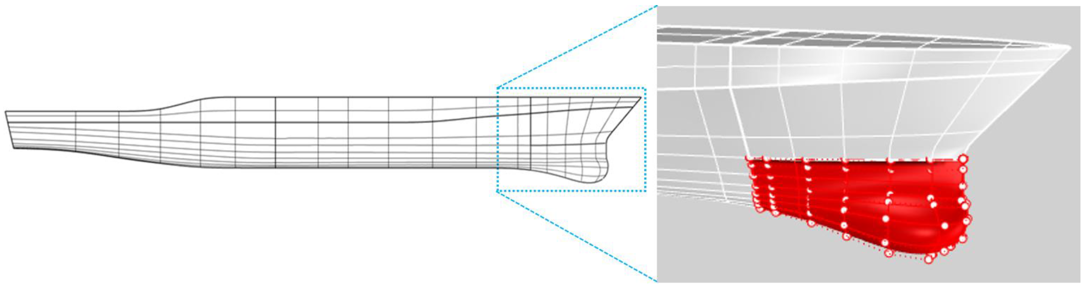
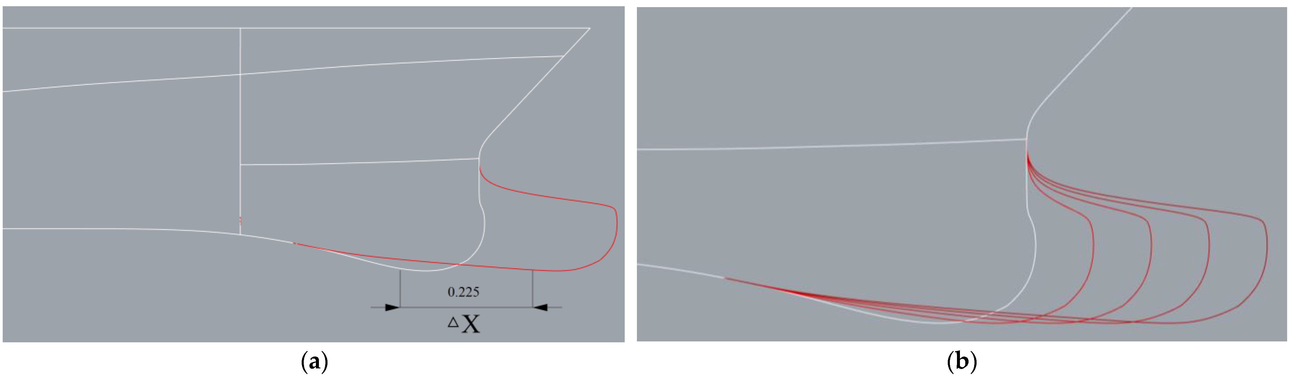
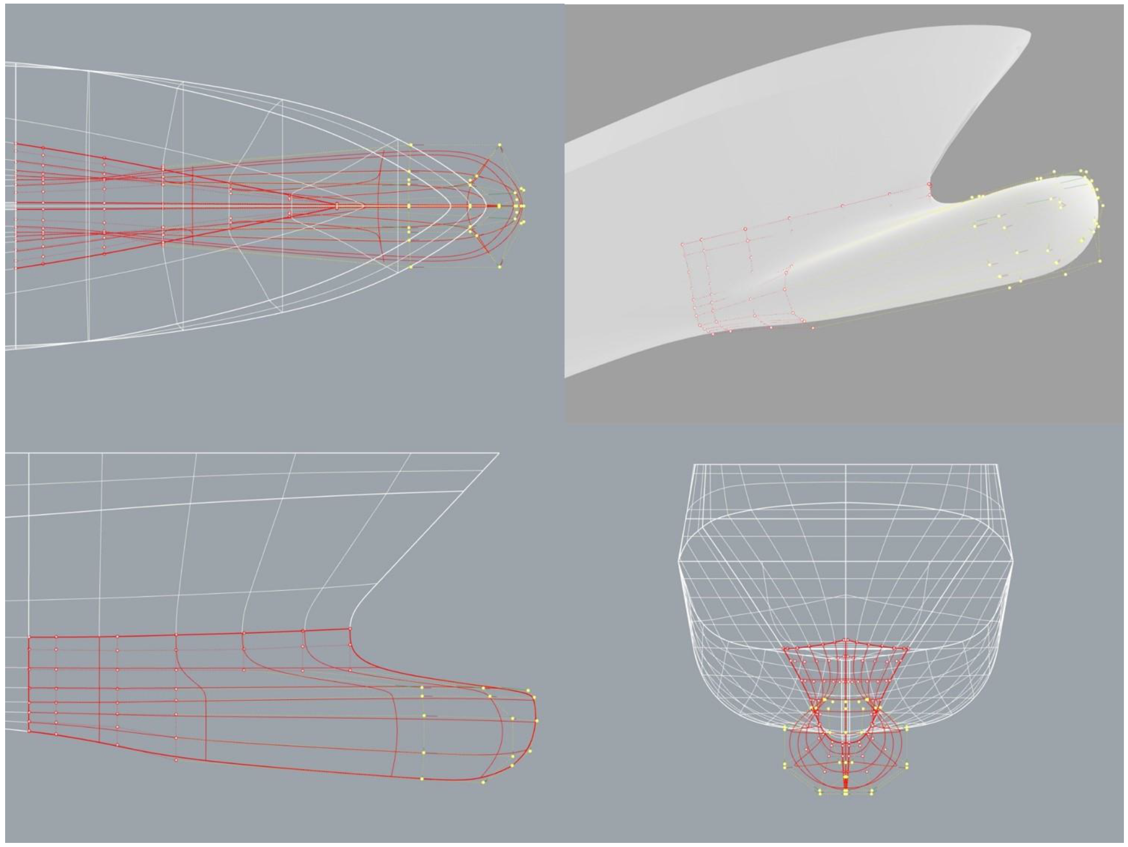
The zoom-in blue frame of Figure 1 shows the main target object in this study: the sonar dome integrated with the ship’s bow. In Figure 1 right, the part in red is the NURBS surface of the sonar dome with the control points (red hollow points). It is an independent part to change the geometry on the ship’s hull, and the other part of hull geometry is fixed. The distribution of the control points around the original sonar dome is illustrated in Figure 2 in detail and multiple views. Among the control points, the yellow hollow points are selected to protrude the dome geometry forward as demonstrated in Figure 3. The protruding distance of all selected control points is defined as and explained in Figure 3a. The range of length variation is = 0–0.24 m. As a result, the different lengths of the sonar dome variations are generated, simulated in the present work, and then compared with the result of the original sonar dome. The nomenclature of the sonar dome variations is and F stands for forward protrusion. For instance, the optimal dome (see Section 4.2) is F0.225 which means the dome with = 0.225 m. The details of the distribution of the control points around the F0.225 dome after the geometry change are displayed in Figure 4. Accordingly, the original sonar dome is identical to F0, i.e., = 0. F0 represents the original sonar dome in the rest of this paper.
3. CFD Methods
The CFD software used to simulate and analyze the viscous flow field around the ship with different sonar domes in this study is version 6 of OpenFOAM (Open-Source Field and Manipulation).
3.1. Numerical Methods and Models
Since the bulbous bow effect is related to the ship-making waves, the free surface effect is modelled by VOF (Volume of Fluid [26]) method for two-phase incompressible flow, i.e., water and air. The turbulent velocity, pressure, and phase distribution were solved by the RANS (Reynolds-averaged Navier–Stokes) and VOF solver interFOAM. The VOF was revised significantly from [26]. The numerical compressibility was treated in the source term for the sharp interface on the free surface [27]. A flux limiter called MULES (multidimensional universal limited explicit solver) was introduced [28]. The turbulence model is SST (shear stress transport) k-ω for SST-2003 version [29,30]. The velocity and pressure coupling approach is PIMPLE [31], exclusively developed for OpenFOAM, and necessary for pseudo-transit simulation in interFOAM. Based on the finite volume method, to integrate the governing equations in the above-mentioned solvers and models, the control point value between two volumes (or two surfaces) is obtained by linear interpolation. The numerical details are listed in Table 2.
The governing equations in the presented work solved by the above-mentioned numerical methods are discussed as follows. The continuity is maintained by Equation (1):
where is the flow velocity. The momentum is conserved by Equation (2):
wherein t is time and is the fluid density. The effective dynamic viscosity consists of the fluid viscosity and turbulent viscosity solved by the SST k-ω model explained in the next paragraph. p is the pressure, is the gravitational acceleration, and is the position vector. In VOF, and , respectively, are composed of water (subscript w) and air (subscript a) through the volume fraction , as shown in Equations (3) and (4):
Through those two equations, the VOF transport equation, i.e., Equation (5) as below, is solved together with Equations (1) and (2) to model the two-phase flow.
with the numerical compressive relative velocity considered.
In the SST k-ω turbulence model, turbulence kinetic energy k and turbulence dissipation rate ω are solved in Equations (6) and (7), respectively:
in which is the production limiter, the strain rate tensor, and the coefficient of thermal expansion. is a hyperbolic tangent function, i.e., tanh, to provide smooth transiting between 0 and 1. = 1 activates the k-ω model inside the boundary layer near the wall, and = 0 switches to the k-ε model in the free stream away from the wall. Thus, the constants in Equations (6) and (7) for k-ω and k-ε models are blended and determined by :
In the end, the solved k and ω provide the turbulence in Equations (1) and (2) through Equation (9) with a second blending function .
3.2. Computational Domain and Grid Topology
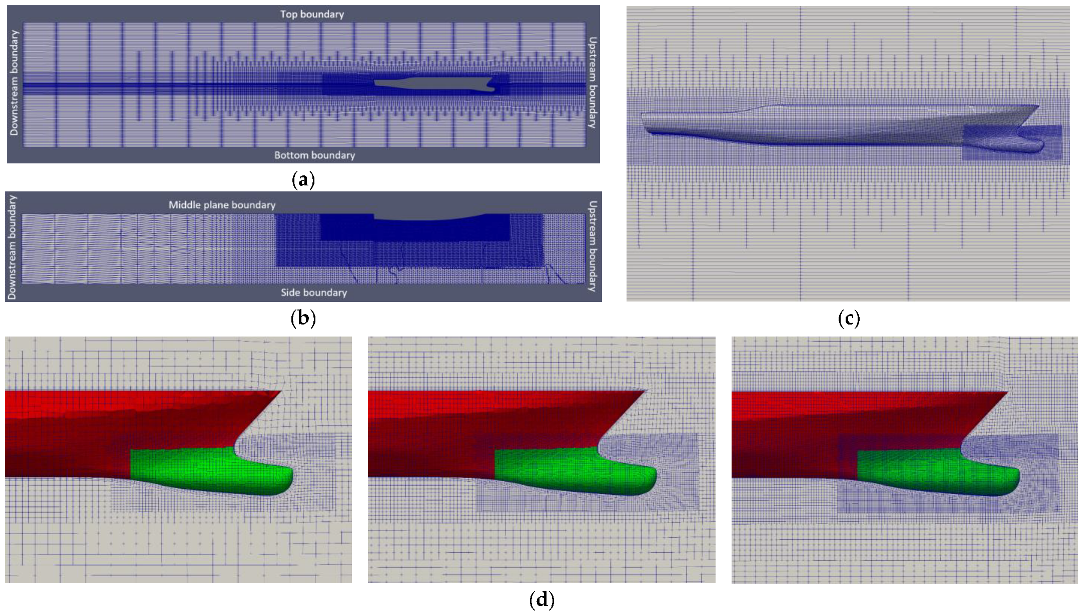
For the computational domain size, the concern is the least influence from truncation error and to refer to the actual dimensions of the towing tank for the model test. The length from ship FP, i.e., the origin (0, 0, 0), to upstream boundary (+x direction) is 1L, and 3L from ship AP, i.e., (L, 0, −t), to downstream boundary. Since the flow field of the port and starboard side is symmetric, only half the computational domain of the starboard side (–y direction) is constructed to save computational time. The undisturbed free surface lies on the z = 0 plane and coincides with the ship’s water plane. The top, bottom, and side boundaries are set 2 m away from the ship’s water and middle plane corresponding to z = 2 m and −2 m, and y = −2 m. The domain size can be seen in Figure 5a,b. The F0.225 dome (found optimal in Section 4.2) is the example of the grid system in Figure 5.
As demonstrated in Figure 5, the grids are distributed finer close to the free surface and hull to capture ship-making waves and resolve flow boundary layer. An additional refinement box is arranged around the sonar dome, as illustrated in Figure 5c, to provide high resolution for the dome geometries and the flow field around them. The grid size in the refinement box is maintained as about 0.01 m vertically, horizontally, and transversely. Across the free surface, the grid size in height is also about 0.01 m. The initial grid is generated by the Cartesian grid method based on the grid distribution on the domain boundaries, and refined level by level from far field to the region around the hull. Finally, the unstructured body-fitted grid on the hull surface is built with hexahedra mainly and the other minor element types. The wall function is employed in the simulation to avoid a large number of fine grids on the solid surface and reduce the computational time. Thus, the non-dimensional thickness of the first layer grid (y+) targets 150 to be within the logarithmic layer range (y+ between 30 and 200) of the boundary layer. Consequently, the three grid layers are generated with about 0.01 m thickness of the first layer. The layers and unstructured grid can be seen clearly on the ship’s bow part in Figure 5d for three different grid sizes: coarse, medium, and fine grid. They are required for the next section analysis to check grid independency and uncertainty of our CFD method.
3.3. Verification and Validation (V&V) Method
The V&V (verification and validation) theory used in this study is based on ITTC 7.5-03-01-01 [32]. First, the CFD resistance value (R) of the ship’s hull with F0 sonar dome is examined for V&V. Next, the verified and validated CFD and grid method are followed to simulate different sonar domes (lengths). The V&V result is discussed in Section 4.1 with the verification for the optimal F0.225 found in Section 4.2.
3.3.1. Verification
Three different grid sizes, i.e., a set of fine (S1), medium (S2), and coarse grids (S3), are built and simulated for grid independence check. The refinement ratio between S3 and S2, S2 and S1 grid, is compiled in each spatial direction of boundaries to generate the initial grid. However, the grid number of unstructured grids involves the generation of different element types. For a Cartesian grid, it depends on refinement levels. Therefore, the final total grid number would not be exactly for the grid number , , on boundaries in x, y, z direction, respectively. Thus, the ratio of total grid number is managed carefully to be as close to as possible. Total grid number for different grid sizes is listed in Table 2.
A ratio RG is suggested as below to evaluate the grid convergence:
If RG < 1 is achieved, it indicates the resistance difference between S2 and S1 grid is less than the difference between S2 and S3 grid, and is so-called monotonic convergence. By increasing grid number, the resistance difference between two different grid sizes is reduced. As a result, the grid independence existing in our CFD method is proven. In other words, our CFD method is verified.
3.3.2. Validation
Grid uncertainty (UG) is computed by the factor of safety method with correction factor [32]. The simulation error (E%D) against experimental data (D) is defined as:
Satisfying |UG| > |E%D| of S1 represents validation is achieved or our CFD method is validated. The comparison between CFD and experimental results is less uncertain, i.e., more confident, than the comparison only for CFD results of different grid sizes.
Since many geometries for different dome lengths need to be simulated, the medium grid is selected to strike a balance between the computational time and flow field solution resolution. The total grid number 1.44 M (million) is maintained for all different dome lengths, e.g., F0.225 described in Table 3. The experiment is only available for F0. The optimal design (F0.225) is chosen to perform the above-mentioned verification analysis to confirm its grid convergence and uncertainty. Table 3 indicates the very subtle difference (less than 0.1%) between F0 and F0.225 grid. Either for F0 or F0.225, the total grid numbers are 4.26 M, 1.44 M, and 0.46 M, respectively, for fine, medium, and coarse grid.
3.4. Boundary Conditions
3.4.1. Upstream, Side, and Bottom Boundary
Except for p = 0 for pressure p, the constant values are specified based on far field and free stream turbulence: inflow velocity u = (U0, 0, 0) m/s, turbulence dissipation rate ω = 2 s−1, turbulence viscosity t = = 0.0000005 m2/s, turbulence kinetic energy k = 0.00015 m2/s2. In VOF, the volume fraction α = 0.5 on the z = 0 plane is defined as the initial location of the free surface. For totally filling with air or water, α = 0 or 1, respectively. As mentioned before (Section 3.2), only starboard flow field is modelled, so the symmetric condition, i.e., , is imposed on the middle plane y = 0.
3.4.2. Top Boundary
For velocity, u = 0 with an inverse flow treatment makes sure only outward velocity is solved. The total pressure is zero, but once inverse flow occurs, zero dynamic pressure is forced. For turbulence viscosity, t= 0. The so-called Inlet Outlet condition is applied: (ω, k, α) = 0, but in case of inverse flow, the constant values of Section 3.4.1 are prescribed.
3.4.3. Downstream Boundary
For velocity, u = 0, but u is automatically adjusted by the average flux of air and water phase if inverse flow happens. For pressure and turbulence viscosity, (p, t) = 0. The Inlet Outlet condition is specified for ω and k. α = 0 for 0 < α < 1. However, to secure 0 < α < 1, α = 0 is forced if α < 0, and α = 1 is limited if α > 1.
3.4.4. Solid Surface Boundary
The no-slip condition is adopted on the ship’s hull and sonar dome surface with the wall function as discussed for y+ in Section 3.2. It is implemented through the following ω and t equation in consideration of surface roughness [33,34]. is the non-dimensional roughness height determined by the sand-grain roughness height KS = 100−6 m.
4. Results
In Section 4.1, the resistance of the ship with the original sonar dome is analyzed to satisfy the V&V requirements, and then the medium grid is selected to study the influence of the sonar dome’s length. The resistance component (Section 4.2), ship waves (Section 4.3), velocity field (Section 4.4), pressure field (Section 4.5), wall shear stress (Section 4.6), and vortex structure (Section 4.6) are investigated to thoroughly understand the details of the bulbous bow effect and the resistance reduction mechanism.
4.1. V&V Analysis
Table 4 presents the total ship resistance R(N) of the F0 sonar dome for S1, S2, and S3, and their errors E%D computed by Equation (11). As the grid number increases, the overpredicted error decreases to be slightly underpredicted. All absolute errors under 4% are quite low. The lowest error is even less than 0.4% (S1 value in Table 4).
For V&V of F0, RG given by Equation (10) is less than 1. Thus, verification and grid independence are achieved. |UG| larger than |E%D| of S1 in Table 4 indicates the validation is accomplished. The UG is the percentage of D. To estimate UG, and / are listed in the table as well. is defined in Equation (10), and is the order of accuracy [32] computed by Equation (14) below. The theoretical accuracy order is 2 here, since the highest order of the numerical methods in the presented work is 2 (Table 2).
reflects our simulation accuracy is close to the second order.
Based on the above-verified and -validated CFD results, the compromise between the time and solution resolution mentioned in Section 3.3.2 and the S2 error is only overpredicted by 1%; the medium grid (S2, total grid number 1.44 M) is our preferred option to study the sonar dome’s length in the next section. F0.225 is the optimal sonar dome with the lowest resistance. For verification, RG < 1 for F0.225 proves the grid is independent. For validation, although F0.225’s experiment is unavailable, UG can be estimated by the percentage of the S1 value with and / in Table 4. Those values are similar between F0 and F0.225, e.g., UG close to 4%, is around 2% of S1 value, and / is in the range of 0.6–0.8 for both sonar domes. In conclusion, the results of F0.225 can be regarded as validated.
In addition, the average y+ result is included in Table 4 for F0 and F0.225. As the logarithmic layer is targeted in Section 3.2, the resultant y+ = 30–200 on average is confirmed for both F0 and F0.225. All y+ is within 154–169.
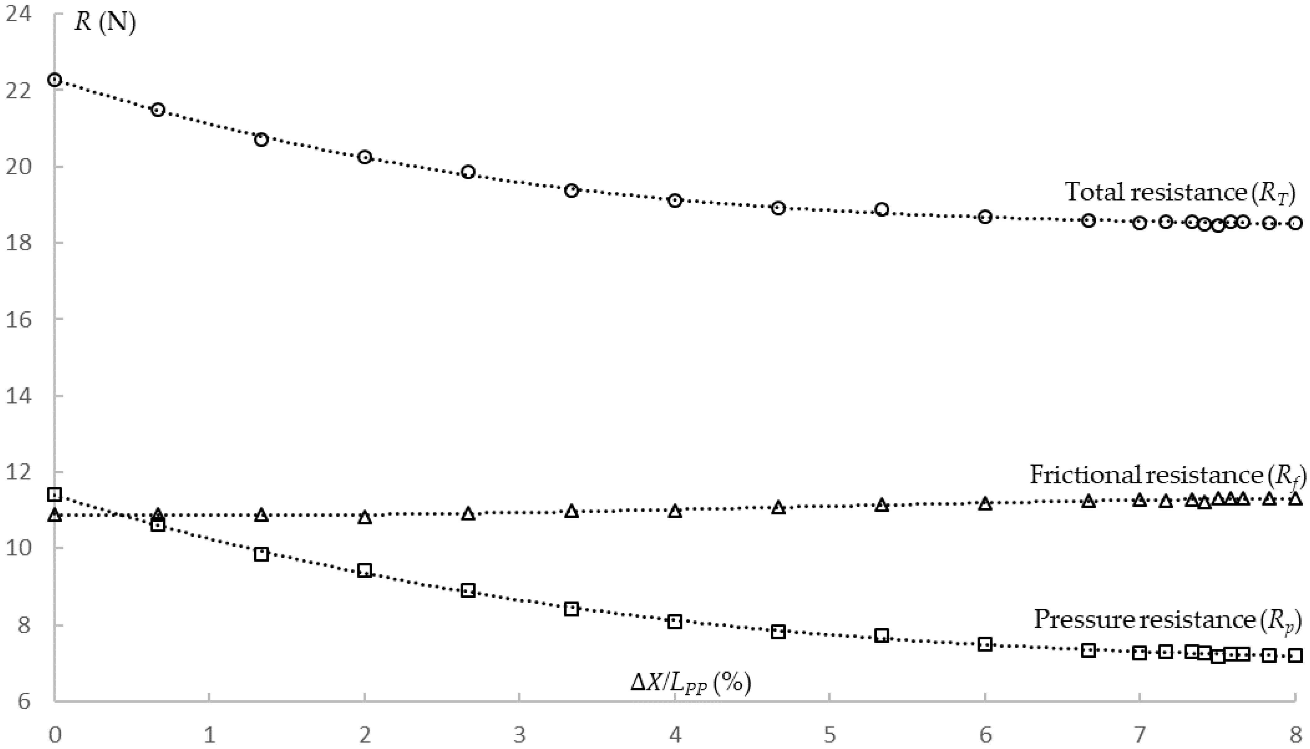
4.2. Resistance for Different Sonar Dome Length
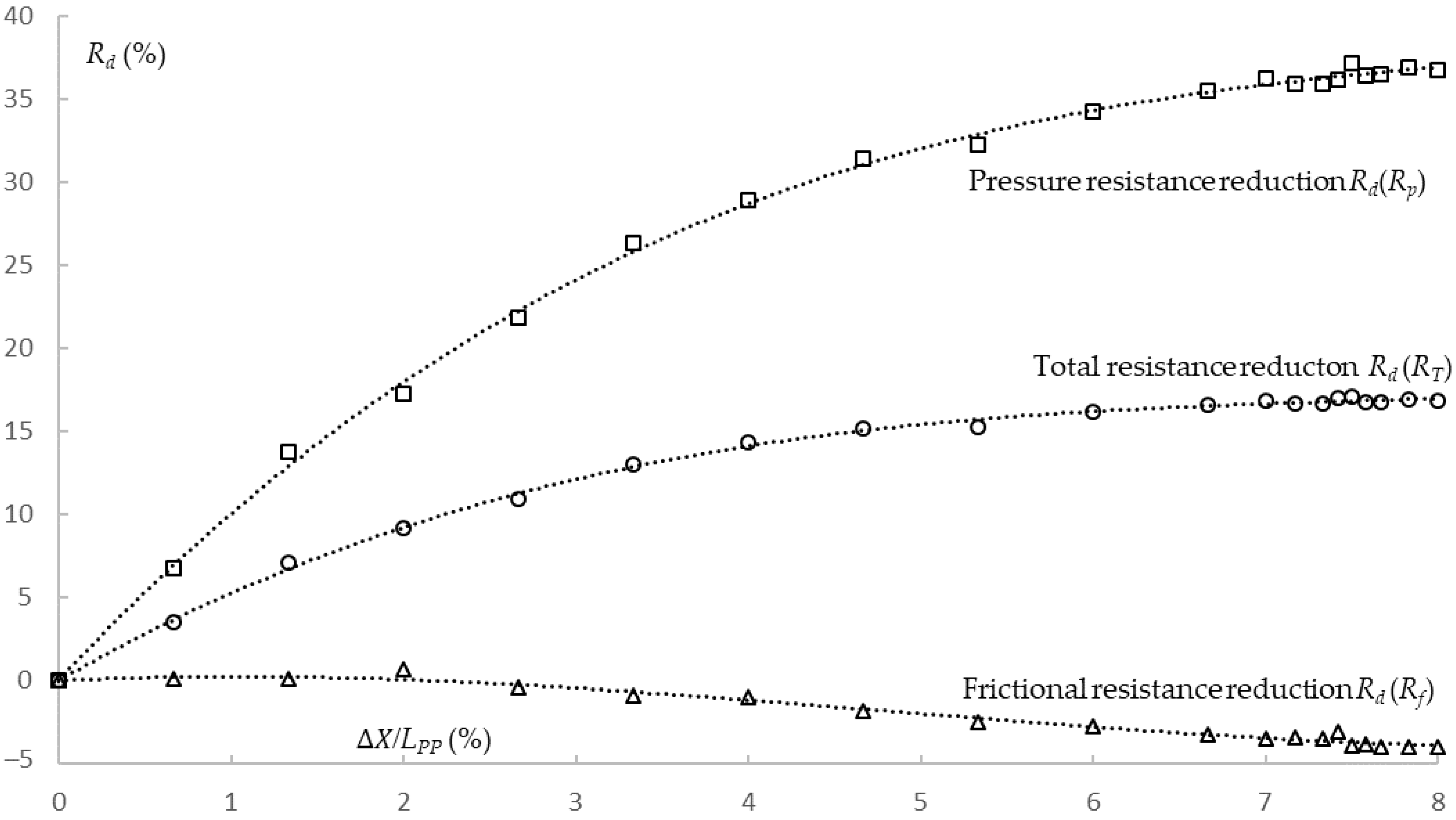
Table 5 shows the resistance result for total resistance (RT) and its components: pressure resistance (Rp) and frictional resistance (Rf). In the table, the ratio /LPP of the sonar dome’s length protruding forward and the ship’s length LPP is also listed as a percentage to give a sense of how long is compared to the whole ship. The trend of RT, Rp, and Rp to /LPP, is drawn in Figure 6, respectively. The resistance reduction Rd of the sonar dome with a different length from F0 is defined as:
As R = (RT, Rp, Rp), the total resistance reduction Rd(RT), pressure resistance reduction Rd(Rp), and frictional resistance reduction Rd(Rf) is calculated, respectively. The trend Rd(RT), Rd(Rp), Rd(Rf) to /LPP, respectively, is drawn in Figure 7.
As the sonar dome length extends longer, the total resistance decreases immediately, i.e., the resistance reduction increases. The increasing trend of Rd(RT) is clear up to F0.21 in Figure 7 (RT decreasing in Figure 6). By further increasing (from F0.215 to F0.24), RT oscillates around 18.5–18.6 N, and Rd(RT) oscillates around 16.7–17%. The optimal dome F0.225, i.e., = 0.225, with lowest R and largest Rd(RT) is found within the range of = 0–0.24 m. Protruding the sonar dome forward 7.5% of the ship’s length can reduce the maximal 17% of the total ship resistance.
For F0, Rp is larger than Rf. Just being slightly longer, such as F0.02, Rp immediately turns out to be smaller than Rf. As keeps increasing, Rp drops significantly from around 11 N to 7 N, and Rd(Rp) increases even more dramatically to more than 36%. For the optimal F0.225, Rd(Rp) reaches 37%. Thus, Rp is the major reason for the resistance reduction. In contrast, only F0.02–0.06 have a lower Rf than F0 has. All the other domes produce a larger Rf, i.e., negative Rd(Rf). In the end, Rf rises slightly less than 0.5 N with around −4% of Rd(Rp) because the wetted area increases for longer sonar domes. The influence of Rf on the resistance reduction is minor. Note that the ship’s length LPP remained the same for all .
4.3. Ship-Making Wave Pattern
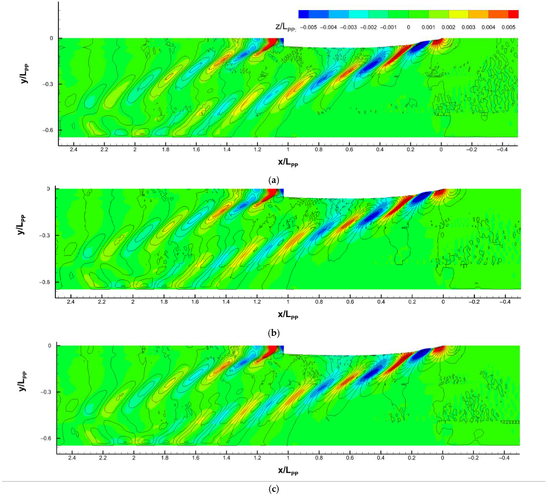
The free surface elevation z, and length in the x and y direction are non-dimensionalized by the ship’s length LPP in this section. The ship-making wave patterns around the ship’s hull with the F0, F0.14, F0.225, and F0.24 domes are described in Figure 8. For the Kelvin wave system [35] of a ship, the diverging waves and wave cusps are clearer than transverse waves. A comparison of Figure 8a–d indicates all wave patterns are very similar, except that the second bow wave crest of F0.14, F0.225, and F0.24 shows discontinuity laterally. For a longer dome length, the wave amplitude is generally smaller. It is more obvious in Figure 9 shown by the zoom-in and larger contour range bounds. The first and second bow crest (trough) occur with lighter red (blue) as the dome length increases. Since F0.225 is the optimal case, its second crest height is lowest, i.e., smallest brown contour area. By measuring the first bow wave crest, z/LPP is larger than 0.01 for F0, but z/LPP is only 0.004–0.006 for F0.225. The wave cancellation related to the ship’s wave-making resistance reduction, i.e., the bulbous bow effect, by F0.225 is confirmed.
By overlapping the waves of each dome design and F0, Figure 10 reveals the stern waves are almost identical. Moreover, the bow and stern wave envelopes of both sonar domes and their angles are consistent. The difference is the phase of the bow waves, which are further examined in Figure 10. From F0.14 to F0.24, the first bow wave crest shifts to a more forward position ahead of F0’s. Eventually, the first bow wave crest of F0 is located between the first wave crest and the trough of F0.225 (or F0.24), i.e., 90-degree phase lag.
Based on the wave theory [36], the ratio of the wave length λ to ship length LPP is:
In our case, Fn = 0.23, so theoretical = 0.332 or 33.2%. In Figure 8a, the first bow crest takes place slightly behind the ship’s FP, i.e., x/LPP = 0, and the second crest appears around x/LPP = 0.3. In Table 5, F0.225 corresponds to /LPP = 7.5%. Thus, in Figure 8d, the first bow crest emerges around x/LPP = −0.75, and the second crest happens around x/LPP = −0.2. Therefore, the wave length of both sonar domes is around 0.3, which agrees with the theoretical value. Furthermore, the 90-degree phase lag is one-quarter wave length. For the wave length 0.3, the one-quarter wave length is 0.075 corresponding to F0.225’s /LPP = 7.5%. It means the bow wave crest is generated above the F0.225 tip, and when propagating to the ship’s FP, the wave is at zero height. The wave after FP turns into a trough and cancels the bow wave crest as F0 has.
In addition, since the towing tank side wall is simulated, in Figure 8, the bow waves reflect on the side around x/LPP = 1.96 for F0, 1.95 for F0.14, and 1.92 for F0.225 and F0.45. The angle between the wave envelope and middle plane can be calculated as around 19 degrees, close to the theoretical value [36]. The theoretical value for the wave length and envelope angle is based on a single point of the moving pressure source. Since the pressure is a distribution along the ship’s surface in our case, the ship-making waves are more complicated.
4.4. Velocity Field around Ship’s Hull and Sonar Dome
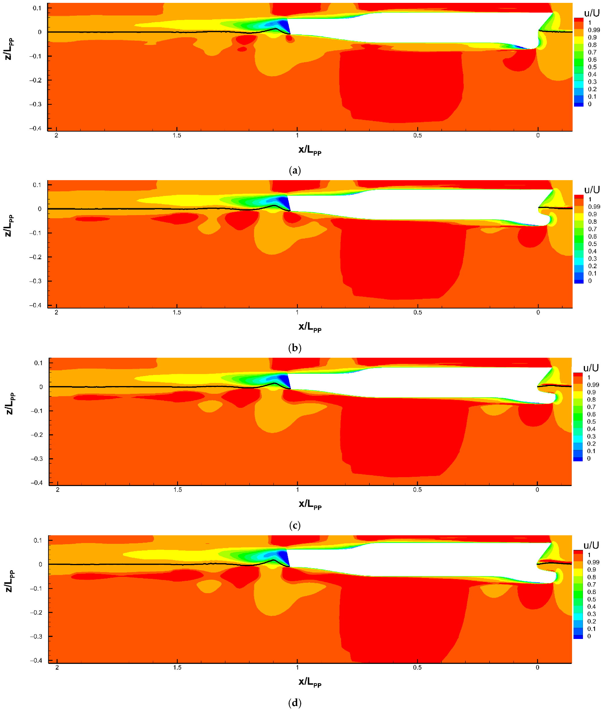
In Figure 11, the axial velocity distribution around the ship’s hull and far field on the middle plane (y = 0) is provided for F0, F0.14, F0.225, and F0.24. The length in x and z direction are non-dimensionalized by the ship’s length LPP. The axial velocity u is non-dimensionalized by the ship’s speed U0.
Compared to F0, the u/U0 > 1 area of F0.14, F0.225, and F0.24 is larger under the ship. Especially for F0.225 and F0.24, the u/U0 > 1 area is continuous under the sonar dome and through the whole ship’s bottom. In the ship’s wake, the u/U0 > 1 area of F0.14, F0.225, and F0.24 develops very long downstream up to around x/Lpp = 1.9. F0.14’s area is smaller and scattered. Instead, the u/U0 > 1 area of F0 is extremely short, and it is just two small fragments around x/Lpp = 1.2. The higher flow acceleration outside the boundary layer (identified by u/U0 = 0.99 contour line) around the ship and higher wake velocity behind the ship are the evidence for F0.225 performing much lower total resistance. From F0 to F0.24, the u/U0 > 1 area becomes larger. The u/U0 > 1 areas of F0.225 and F0.24 are similar. This trend is consistent with the decreasing resistance trend to nearly a constant discussed in Section 4.2 and in Figure 6.
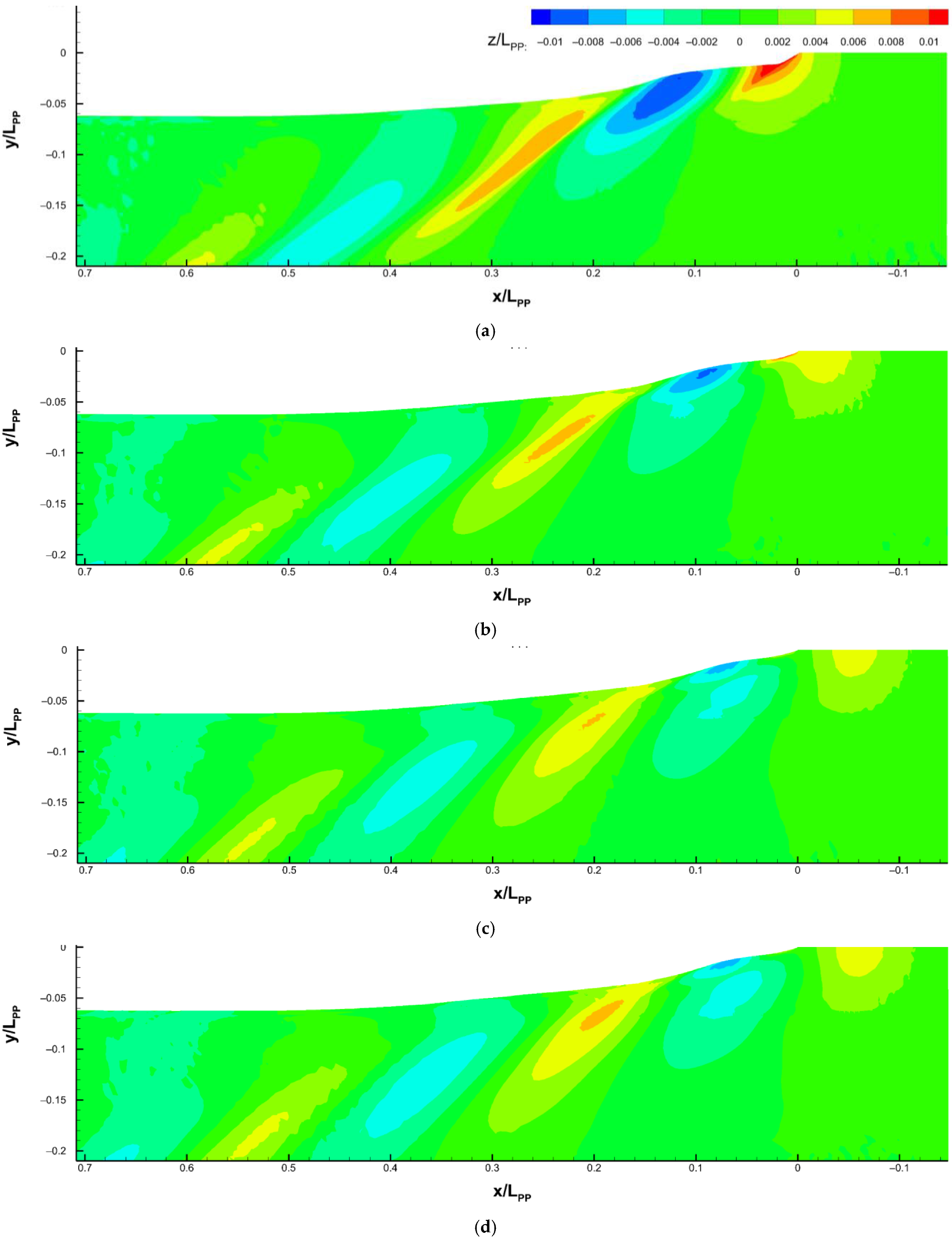
The zoom-in velocity flow field including u/U0 distribution and vector field (u/U0, w/U0) in Figure 12 illustrates the flow separation behind the sonar domes. In comparison with the other sonar domes, the separation area of F0 is very large with an obvious reverse flow, i.e., u/U0 < 0, and the vectors point opposite to the inflow direction. For F0.225 and F0.24, the separation area is remarkably smaller and thinner, and the reverse flow either does not form or is extremely vague. On F0.14, an area with u/U0 < 0 (dark blue) is still observable but much smaller than F0’s. The boundary layer thickness of F0.14, F0.225, and F0.24 is relatively thin as well. Using the u/U0 = 0.99 contour line as the indicator, check the location it intersects at x/Lpp = 0.17 line, i.e., the vertical axis in the left of Figure 12. It is around z/Lpp = −0.076 for F0. The intersection is −0.07 for F0.14, and −0.066 for F0.225 and F0.45. This local flow field improvement benefits from the less steep back slope of F0.14, F0.225, and F0.24 since the sonar dome is longer under the same depth. It supports the trend of pressure resistance reduction discussed in Section 4.2. The smaller separation implies the smaller pressure difference between the front and back surface of the sonar dome. In conclusion, F0.225 is not only functional in the same way as a bulbous bow to cancel waves, but the viscous flow behavior around the sonar dome is also much improved.
4.5. Pressure Distribution around Ship’s Bow
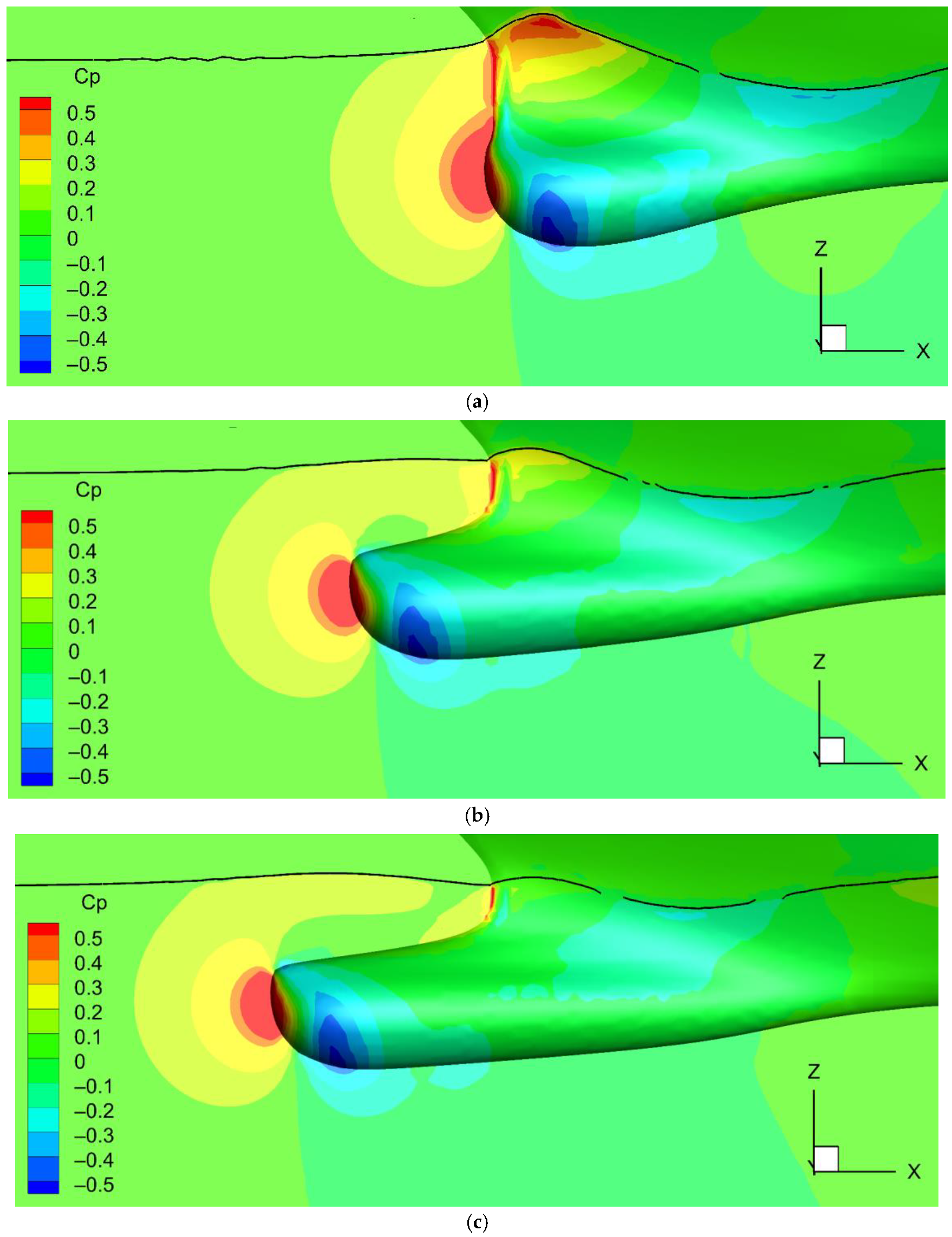
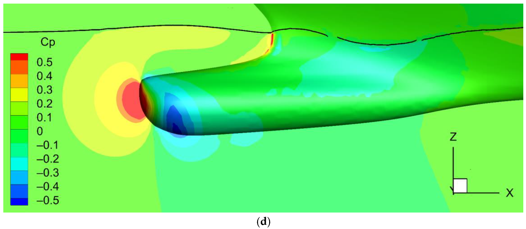
The pressure coefficient Cp in the flow field and on the surface is calculated as below:
The Cp distribution around the ship’s bow and sonar dome is plotted in Figure 13 for F0, F0.14, F0.225, and F0.24. The high pressure, e.g., Cp > 0.5 (in red color), covers a larger area in front of the F0 sonar dome tip along the whole leading edge of the ship’s bow. The free surface profile in Figure 13 also points out that F0 generates a larger bow wave crest (also observed in Section 4.3). As the crest rises upward and hits the ship’s bow flare, the high pressure with the main part of Cp > 0.4 (in orange color) and tiny part of Cp > 0.5 (in red color) exerts on the hull surface above the sonar dome. Oppositely, the high-pressure area and bow wave crest are relatively small for F0.14, F0.225, and F0.24. There is no high pressure concentrated on the bow flare of F0.225 and F0.24. For F0.14, there is a slightly high Cp (> 0.2) on its flare since its bow wave crest is higher than F0.225’s and F0.24’s. It is the explanation for the high-pressure resistance of F0 and the significant resistance reduction of F0.225 discussed in Section 4.2 for Figure 7. It is the consequence of the combination of the high pressure on the F0.225 (bow flare) being lower and low pressure on the dome back being higher (small separation in Section 4.4). The resultant pressure difference is smaller between them.
4.6. Distribution of Wall Shear Stress on Ship’s Bow
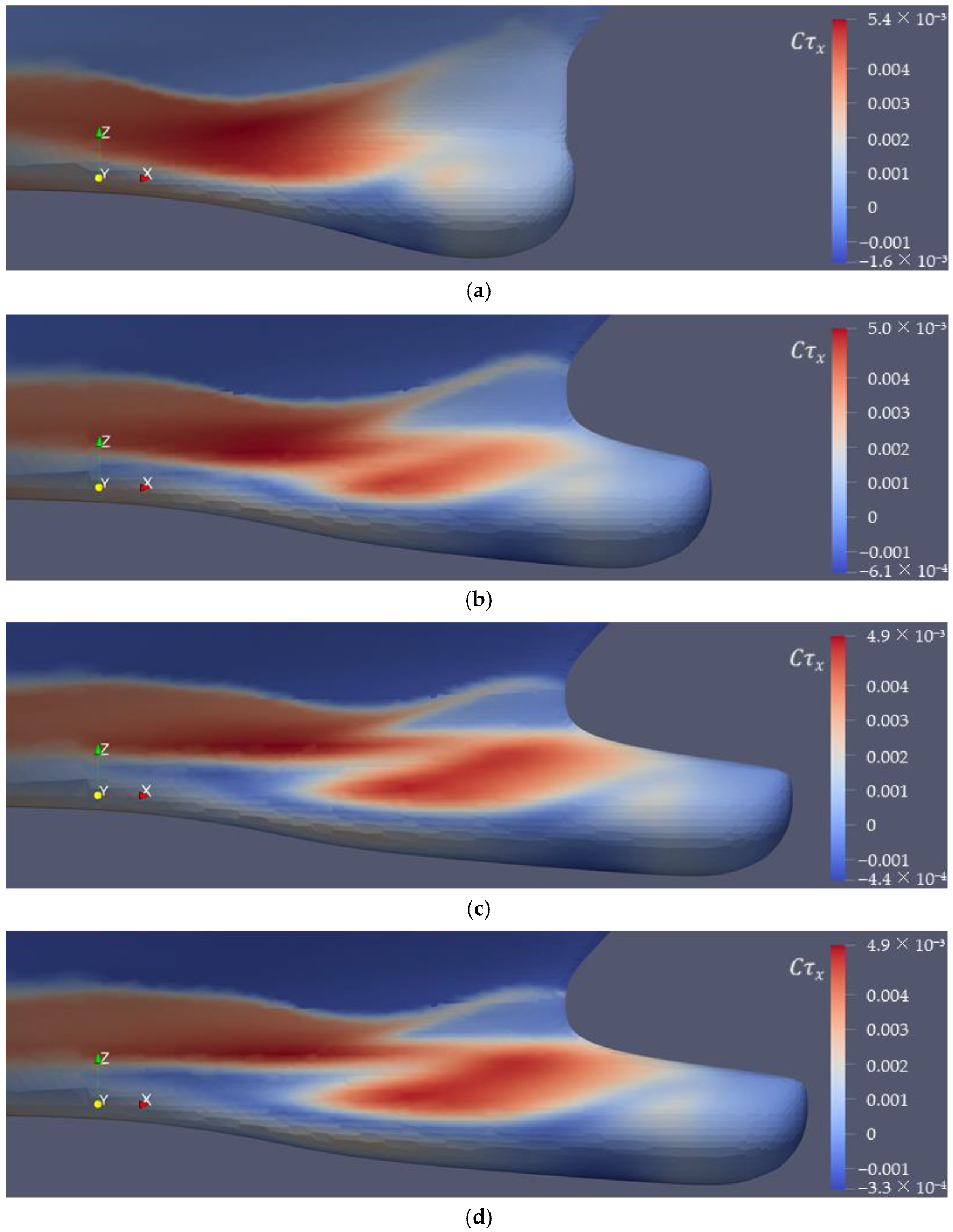
The x component of wall shear stress is non-dimensionalized as below:
The distribution around the ship’s bow and sonar dome is plotted in Figure 14 for F0, F0.14, F0.225, and F0.24. The contour range is the maximal and minimal value on the solid surface. For all sonar domes, the high + reaches around 0.005, which is colored by red in the figure. The high + is generated downstream of the bow wave crest (under the first trough). However, for F0.14, F0.225, and F0.24, an additional large high + area appears under the bow wave crest attached on the upper rear part of the dome. The areas of F0.225 and 0.24 is even larger than F0.14’s. This is the reason the slightly increasing trend of frictional resistance for longer sonar dome lengths was found in Section 4.2 and Figure 6.
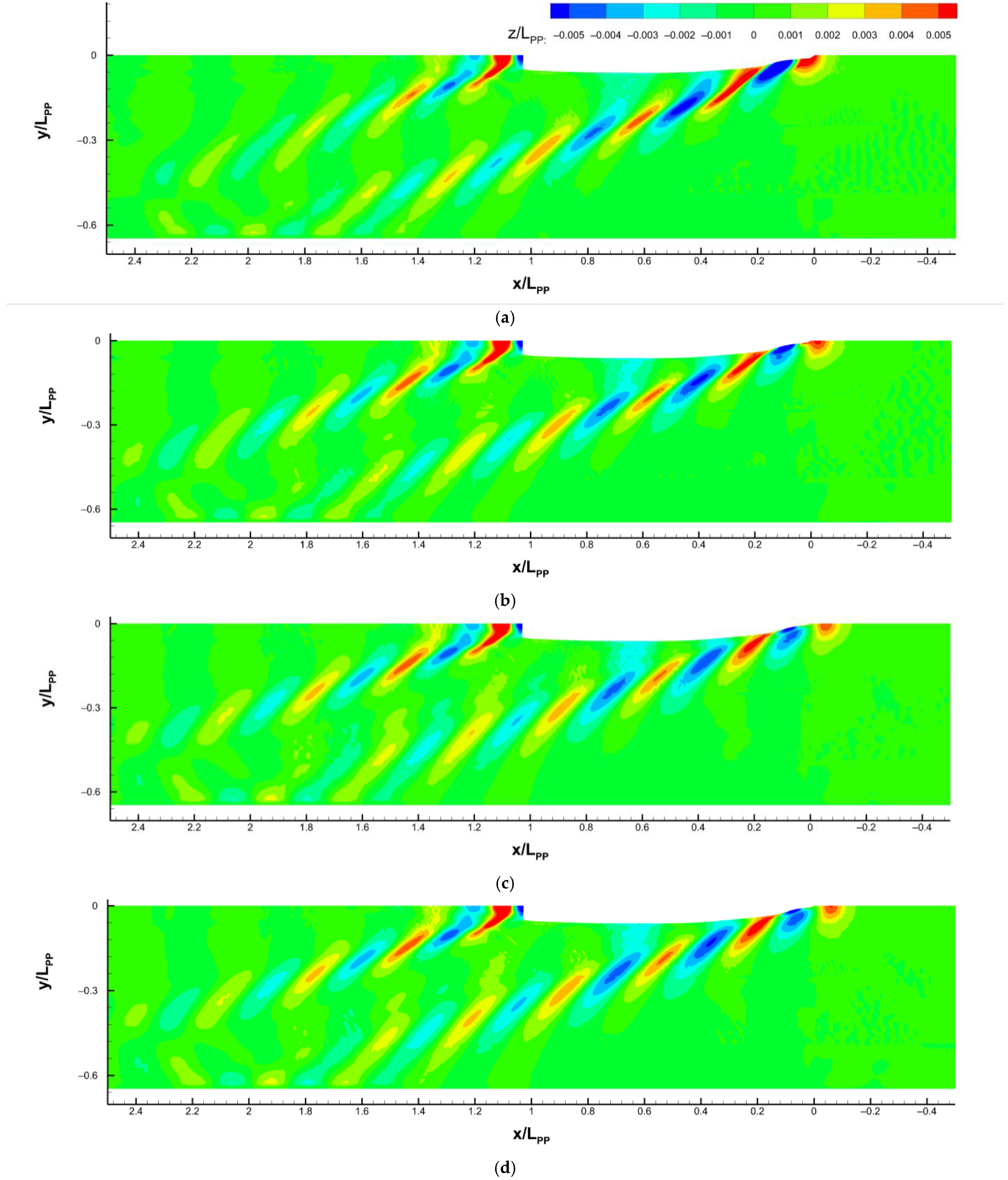
4.7. Vortical Structures around Sonar Dome
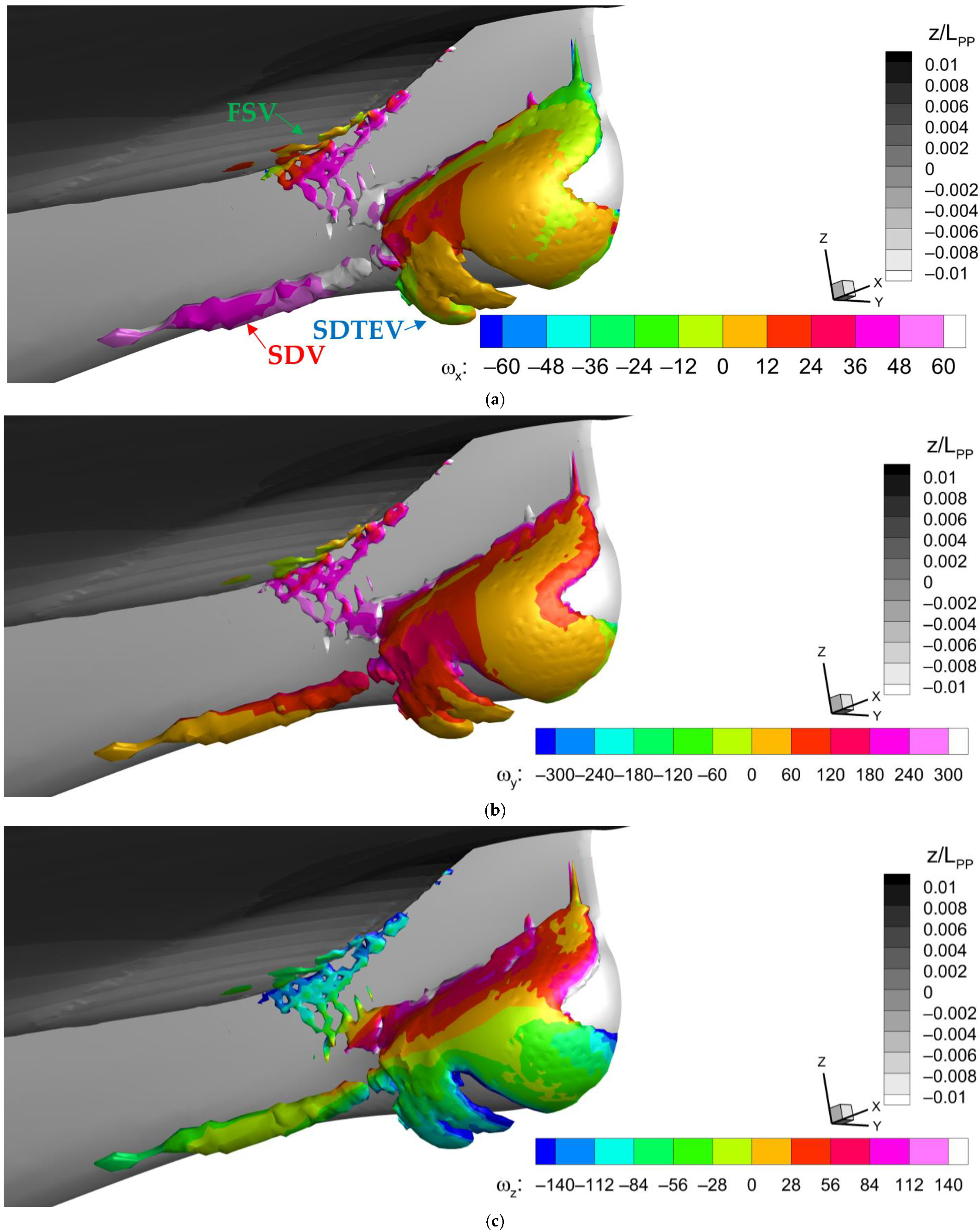
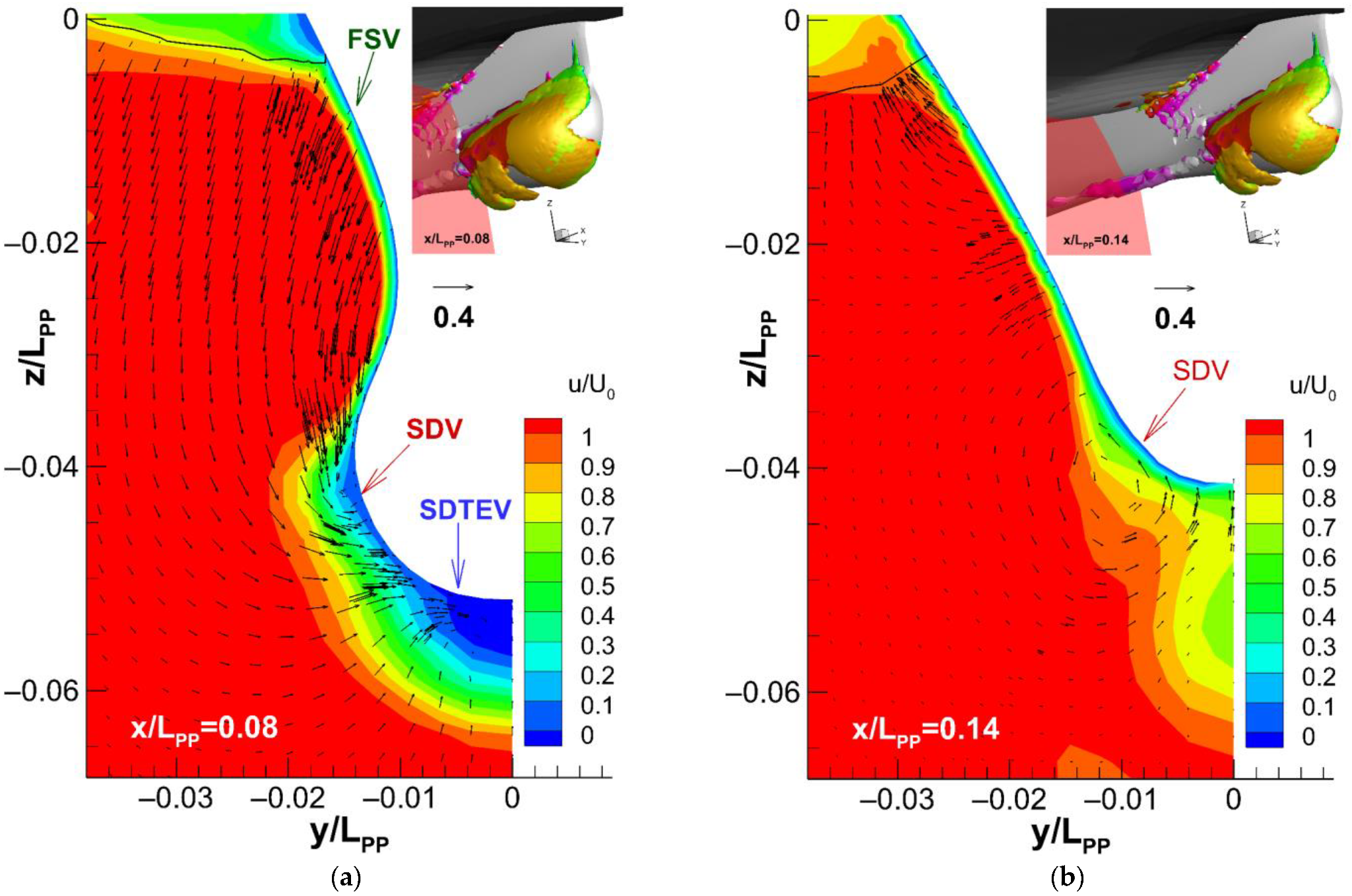
To understand the vortical structures around the sonar dome, Q-criterion [37] based on non-dimensional velocities is applied in this section. For F0, the isosurface of Q = 500 covered by the color flooded contour of ωx, ωy, and ωz is illustrated, respectively, in Figure 15a–c to indicate the flow rotational direction. The ωx, ωy, and ωz are the non-dimensional vorticities in the x, y, and z direction. As pointed out in Figure 15a, several kinds of vortex can be observed and categorized: SDV = sonar dome (side or tip) vortex, SDTEV = sonar dome trailing edge vortex, and FSV = free surface vortex. To examine the vortex phenomena, the axial velocity (u/U0) distribution and vector field (v/U0, w/U0) around the F0 sonar dome are plotted on the x/Lpp = 0.08 plane in Figure 16a and the x/Lpp = 0.14 plane in Figure 16b. SDV and SDTEV are the major phenomena that were also explored in [38,39] for the DTMB 5415 hull, and the terminology of [38,39] is adopted here.
The SDV is induced from both sides of the sonar dome by the downward flow, as shown in Figure 16a. It is also a tip vortex, which is opposite to a wingtip vortex with lift direction upward. After the SDV is detached from the sonar dome, it travels downstream as in Figure 16b. The SDV would extend downstream very far as shown in Figure 15.
The SDTEV results from the flow separation behind the sonar dome back slope, i.e., the trailing edge, as discussed in Section 4.4 and Figure 12. The region of ωy = 0–60 on the SDTEV in Figure 15b agrees with the vector direction of the reverse flow in Figure 12a. In Figure 15c, the high −ωz on the SDTEV indicates the cross-flow rotation inside the flow separation exists, which is induced by the SDV. As shown in Figure 16a, the SDV rotates counter-clockwise, and correspondingly, the SDTEV rotates clockwise into the separation area (in dark blue). The SDTEV does not last long. It is much shorter than the SDV as presented in Figure 15. Moreover, in Figure 16b, only the sonar dome wake is left beneath the ship’s bottom.
The FSV is observed under the bow wave crest in Figure 15, which results from the wave orbital motion. The high downward velocity under the free surface can be seen in Figure 16a, which would produce high vorticity along the bow flare surface below the wave crest as illustrated in Figure 15.
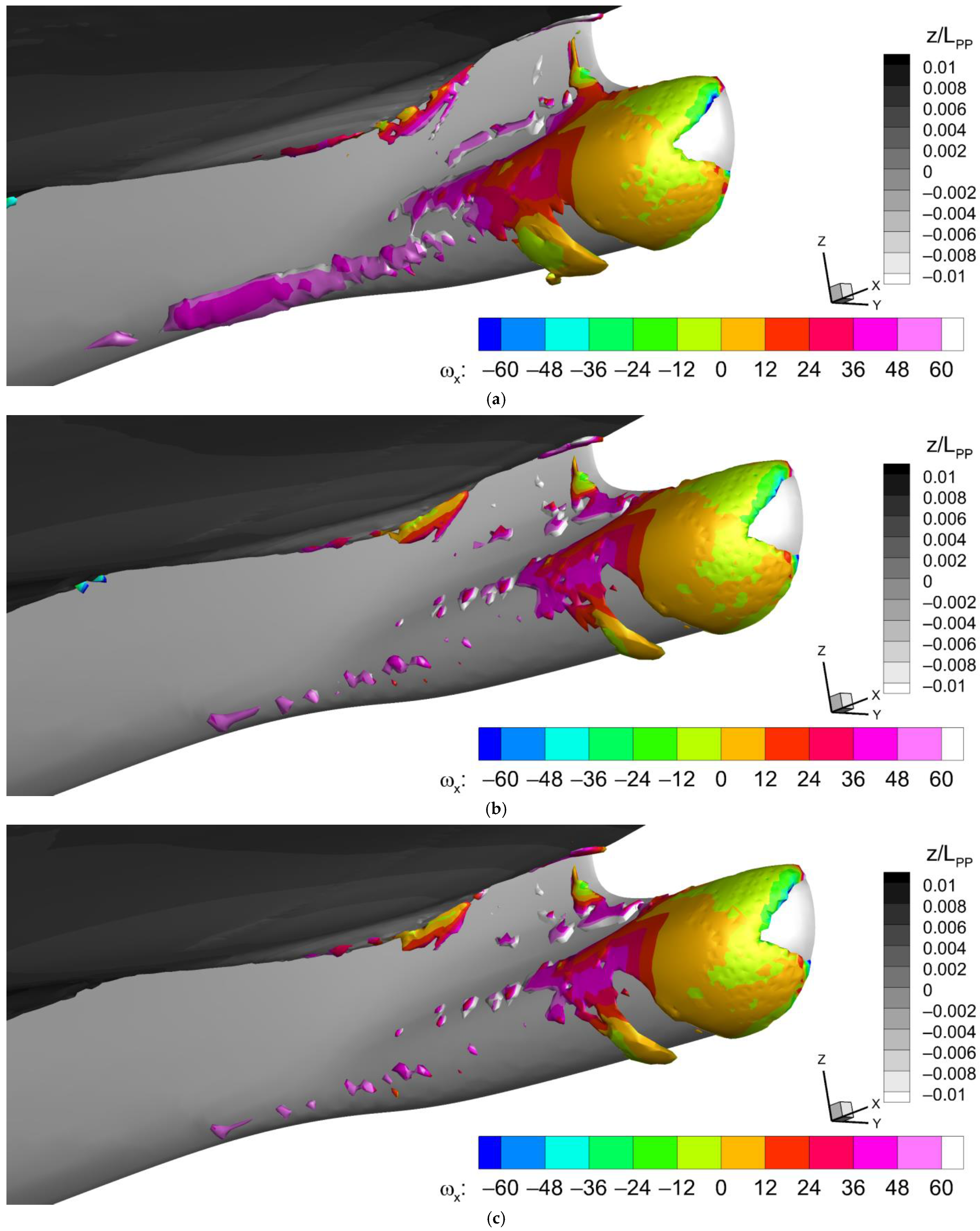
To investigate the effect of the sonar dome’s length on the vortical structures, the same layout of Figure 15a is plotted for the F0.14, F0.225, and F0.24 sonar domes in Figure 17. Compared with F0 in Figure 15a, the difference and improvement caused by F0.225 (Figure 17b) and F0.24 (Figure 17c) is evident. Their SDTEVs are only around half the size (or length), which correlates with the improvement in flow separation found in Section 4.4 and Figure 12. Their SDVs are almost eliminated (under Q = 500) with only scatter distribution remaining. As shown in Figure 17a, F0.14’s performance is between those of F0 and F0.225/F0.24. Its SDTEV is slightly smaller than F0’s and the SDV is still almost as long as F0’s. The FSV still occurs on F0.14, F0.225, and F0.24, but the high vorticity along the bow flare surface disappears. Moreover, another FSV is discovered around the ship’s FP, i.e., the location of the ship’s bow leading edge piercing the free surface. There is no sign of this kind of FSV on F0.
5. Discussion
The analysis and design tool used to determine ship resistance and viscous flow around a ship with different lengths of sonar domes in this proposed work was OpenFOAM. In the first stage, the CFD grid and method for the original sonar dome were simulated, and its results were verified and validated successfully for a ship’s total resistance. In the second stage, in balance with computational time consumption and flow field resolution, the medium grid with 1.44 M grids was selected to study different sonar dome lengths and the bulbous bow effect. The optimal dome was found with 0.225 m forward protrusion and achieved the lowest total resistance, which mainly resulted from the pressure resistance decrease.
The finding is supported by the results of Tahara et al. [40]. A sonar dome for the DTMB (David Taylor Model Basin) 5415 with 7.8% resistance reduction was designed by [40]. The dome length is 39.5% longer than the original geometry.
For the optimal sonar dome, the flow field analysis proved it is not only functional similarly to a bulbous bow by cancelling the bow waves, but also its viscous flow behavior around the sonar dome is much improved. By elongating the dome forward around one-quarter of the ship-making wave length, the maximal bulbous bow effect occurs. The bow wave amplitude was reduced with a 90 deg phase lag. The higher flow acceleration outside the boundary layer around the ship and higher ship wake velocity correspond to the lower total resistance. The following phenomena contribute to the decrease in pressure. The smaller flow separation area, no reverse flow, and thinner boundary layer are observed behind the sonar dome because of its less steep back slope. As a result, the sonar dome’s trailing edge vortex is also suppressed. The high pressure covers a smaller area around the surface of the ship’s bow. The smaller bow wave crest causes no high pressure on the ship’s flare. The sonar dome’s vortex is much improved as well.
In conclusion of the presented work, a sonar dome with a bulbous bow effect is successfully designed and proposed. To achieve 17% resistance reduction, the protruding length of the sonar dome is 7.5% of the ship’s length. The flow field analysis supports that the ship’s bow wave is indeed cancelled and reduced by the forward protruding sonar dome.
For future work, the model ship experiment for the optimal sonar dome design will be suggested. The limitation of the optimal design is that it may only be suitable for one ship speed, i.e., cruise speed, or a range of ship speeds. For the sonar dome’s length to result in a proper bulbous bow effect, it should be inspected for different ship speeds since the ship-making wave length is a function of a ship’s speed. Furthermore, the structural strength and slamming load should be examined for this kind of long sonar dome. The impact of sonar dome length on the internal space and limitation to install the sonar and surrounding instruments should be considered. The bulbous bow effect in waves and its influence on a ship’s seakeeping performance will be investigated as well. To minimize the user’s subjective operation and be more theoretically justified for shape change, a parameterized modeling approach will be developed.
For the possible engineering application, once the desired sonar dome length is decided based on the other limits or concerns, the corresponding resistance reduction can be estimated directly according to our result. The verified and validated CFD method and grid system for the original sonar dome, and the design procedure using CFD proposed in this work can be extended and applied for other ship designs. The detailed flow field analysis also provides the insight and concept for ship and sonar dome design. For instance, to avoid the waves hitting the bow flare causing an increase in resistance, we can either re-design the flare or adopt a wave cancellation mechanism such as the bulbous bow concluded in this work.
Author Contributions
Conceptualization, C.-I.W.; methodology, P.-C.W.; software, P.-C.W.; validation, J.-Y.C.; formal analysis, P.-C.W.; investigation, J.-Y.C.; resources, C.-I.W.; data curation, J.-Y.C.; writing—original draft preparation, P.-C.W.; writing—review and editing, P.-C.W.; visualization, J.-Y.C.; supervision, C.-I.W.; project administration, J.-T.L.; funding acquisition, J.-T.L. All authors have read and agreed to the published version of the manuscript.
Funding
The authors would like to thank the National Science and Technology Council (NSTC) for their support of the project [111-2221-E-006-153]. It was thanks to the generous patronage of the NSTC that this study has been smoothly performed.
Data Availability Statement
Not applicable.
Conflicts of Interest
The authors declare no conflict of interest.
References
- Molland, A.F.; Turnock, S.R.; Hudson, D.A. Ship Resistance and Propulsion, 1st ed.; Cambridge University Press: New York, NY, USA, 2017; pp. 323–327. [Google Scholar]
- Wigley, W.C.S. The theory of the bulbous bow and its practical application. Trans. North East Coast Inst. Eng. Shipbuild. 1936, 52, 1935–1936. [Google Scholar]
- Steele, B.N.; Pearce, G.B. Experimental determination of the distribution of skin friction on a model of a high speed liner. Trans. R. Inst. Nav. Arch. 1968, 110, 79–100. [Google Scholar]
- Shearer, J.R.; Steele, B.N. Some aspects of the resistance of full form ships. Trans. R. Inst. Nav. Arch. 1970, 112, 465–486. [Google Scholar]
- Ferguson, A.M.; Dand, I.W. Hull and bulbous bow interaction. Trans. R. Inst. Nav. Arch. 1970, 112, 421–441. [Google Scholar]
- BSRA. Methodical series experiments on single-screw ocean-going merchant ship forms. Extended and revised overall analysis. BSRA Rep. NS 333 1971, 89, 85–95. [Google Scholar]
- Moor, D.I. Resistance and propulsion properties of some modern single screw tanker and bulk carrier forms. Trans. R. Inst. Nav. Arch. 1975, 117, 201–204. [Google Scholar]
- Kracht, A.M. Design of bulbous bows. Trans. Soc. Nav. Arch. Mar. Eng. 1978, 86, 197–217. [Google Scholar]
- Hoyle, J.W.; Cheng, B.H.; Hays, B. A Bulbous Bow Design Methodology for High-Speed Ships. Soc. Nav. Arch. Mar. Eng.-Trans. 1986, 94, Preprint No. 1. [Google Scholar]
- Castro, R.A.; Azpíroz, J.J.A.; Fernández, M.M. El Proyecto Basico del Buque Mercante, 2nd ed.; Fondo Editorial de Ingeniería Naval: Madrid, Spain, 1997; pp. 1–655. (In Spanish) [Google Scholar]
- Park, A.S.; Lee, Y.G.; Kim, D.D.; Yu, J.W.; Ha, Y.J.; Jin, S.H. A study on the resistance reduction of G/T 190ton class main vessel in Korean large purse seiner fishing system. J. Soc. Nav. Arch. Korea 2012, 49, 367–375. (In Korean) [Google Scholar] [CrossRef] [Green Version]
- Holtrop, J. A statistical re-analysis of resistance and propulsion data. Int. Shipbuild. Prog. 1984, 31, 272–276. [Google Scholar]
- Watson, D.G.M. Practical Ship Design; Elsevier Science: Oxford, UK, 1998. [Google Scholar]
- Liao, P.; Song, W.; Du, P.; Feng, F.; Zhang, Y. Aerodynamic Intelligent Topology Design (AITD)-A Future Technology for Exploring the New Concept Configuration of Aircraft. Aerospace 2023, 10, 46. [Google Scholar] [CrossRef]
- Liao, P.; Song, W.; Du, P.; Zhao, H. Multi-fidelity convolutional neural network surrogate model for aerodynamic optimization based on transfer learning. Phys. Fluids 2021, 33, 127121. [Google Scholar] [CrossRef]
- Liu, X.; Zhao, W.; Wan, D. Hull form optimization based on calm-water wave drag with or without generating bulbous bow. Appl. Ocean Res. 2021, 116, 102861. [Google Scholar] [CrossRef]
- SEA-Japan, No. 303. Available online: https://www.jsea.or.jp/wp_2022/wp-content/uploads/2015/06/Sea303.pdf (accessed on 1 February 2004).
- Hirota, K.; Matsumoto, K.; Takagishi, K.; Orihara, H.; Yoshida, H. Verification of ax-bow effect based on full scale measurement. J. Kansai Soc. Nav. Arch. Jpn. 2004, 241, 33–40. (In Japanese) [Google Scholar]
- Sadat-Hosseini, H.; Wu, P.C.; Carrica, P.M.; Kim, H.; Toda, Y.; Stern, F. CFD verification and validation of added resistance and motions of KVLCC2 with fixed and free surge in short and long head waves. Ocean Eng. 2013, 59, 240–273. [Google Scholar] [CrossRef]
- Yang, K.K.; Kim, Y. Numerical analysis of added resistance on blunt ships with different bow shapes in short waves. J. Mar. Sci. Technol. 2017, 22, 245–258. [Google Scholar] [CrossRef] [Green Version]
- Le, T.-K.; He, N.V.; Hien, N.V.; Bui, N.-T. Effects of a Bulbous Bow Shape on Added Resistance Acting on the Hull of a Ship in Regular Head Wave. J. Mar. Sci. Eng. 2021, 9, 559. [Google Scholar] [CrossRef]
- Cusanelli, D.S.; Karafiath, G. Combined Bulbous Bow and Sonar Dome for a Vessel. U.S. Patent No. US 52,80,761, 25 January 1994. [Google Scholar]
- Cusanelli, D.S.; Karafiath, G. Hydrodynamic Energy Savings Enhancements for DDG 51 Class Ships. In Proceedings of the ASNE (American Society of Naval Engineers) Day, Crystal City, Arlington, VA, USA, 9–10 February 2012. [Google Scholar]
- Sharma, R.; Sha, O.P. Hydrodynamic Design of Integrated Bulbous Bowl sonar Dome for Naval Ships. Def. Sci. J. 2005, 55, 21–36. [Google Scholar] [CrossRef] [Green Version]
- Kandasamy, M.; Wu, P.C.; Zalek, S.; Karr, D.; Bartlett, S.; Nguyen, L.; Stern, F. CFD based hydrodynamic optimization and structural analysis of the hybrid ship hull. Trans. Soc. Nav. Arch. Mar. Eng. 2014, 122, 92–123. [Google Scholar]
- Hirt, C.W.; Nichols, B.D. Volume of Fluid Method for the Dynamics of Free Boundaries. J. Comput. Phys. 1981, 39, 201–225. [Google Scholar] [CrossRef]
- Rusche, H. Computational Fluid Dynamics of Dispersed Two-Phase Flows at High Phase Fractions. Ph.D. Thesis, Imperial College London, London, UK, December 2002. [Google Scholar]
- Graveleau, M. Pore-Scale Simulation of Mass Transfer across Immiscible Interfaces. Master’s Thesis, Stanford University, Stanford, CA, USA, June 2016. [Google Scholar]
- Menter, F.R.; Kuntz, M.; Langtry, R. Ten years of industrial experience with the SST turbulence model. In Proceedings of the 4th International Symposium on Turbulence, Heat and Mass Transfer, Antalya, Turkey, 12–17 October 2003. [Google Scholar]
- OpenFOAM User Guide. Available online: https://www.openfoam.com/documentation/guides/latest/doc/guide-turbulence-ras-k-omega-sst.html (accessed on 5 March 2023).
- Holzmann, T. The numerical algorithms: SIMPLE, PISO and PIMPLE. In Mathematics, Numerics, Derivations and OpenFOAM®; Holzmann CFD: Loeben, Germany, 2006; pp. 93–121. [Google Scholar]
- ITTC-Quality Manual 7.5-03-01-01, CFD General. Uncertainty Analysis in CFD Verification and Validation Methodology and Procedures. ITTC Recommended Procedures and Guidelines. Available online: https://ittc.info/media/4184/75-03-01-01.pdf (accessed on 31 January 2023).
- Liu, F. A thorough description of how wall functions are implemented in OpenFOAM. In Proceedings of the CFD with OpenSource Software, Chalmers University of Technology, Gothenburg, Sweden, 22 January 2017. [Google Scholar]
- OpenFOAM User Guide. Available online: https://www.openfoam.com/documentation/guides/latest/doc/guide-bcs-wall-turbulence-nutkRoughWallFunction.html (accessed on 31 January 2023).
- Kelvin, L. On the waves produced by a single impulse in water of any depth. Proc. R. Soc. Lond. 1887, 42, 80–83. [Google Scholar]
- Newman, J.N. Marine Hydrodynamics, 1st ed.; The MIT Press: Cambridge, MA, USA, 1977; pp. 237–320. [Google Scholar]
- Jeong, J.; Hussain, F. On the identification of a vortex. J. Fluid Mech. 1995, 285, 69–94. [Google Scholar] [CrossRef]
- Bhushan, S.; Xing, T.; Visonneau, M.; Wackers, J.; Deng, G.; Stern, F.; Larsson, L. Post workshop computations and analysis for KVLCC2 and 5415. In Numerical Ship Hydrodynamics, 1st ed.; Larsson, L., Stern, F., Visonneau, M., Eds.; Springer: Dordrecht, The Netherlands, 2014; pp. 286–318. [Google Scholar]
- Bhushan, S.; Carrica, P.; Yang, J.; Stern, F. Scalability studies and large grid computations for surface combatant using CFDShip-Iowa. Int. J. High Perform. Comput. Appl. 2011, 25, 466–487. [Google Scholar] [CrossRef]
- Tahara, Y.; Norisada, K.; Yamane, M.; Takai, T. Development and demonstration of CAD/CFD/optimizer integrated simulation-based design framework by using high-fidelity viscous free-surface RANS equation solver. J. Jpn. Soc. Nav. Archit. Ocean Eng. 2008, 7, 171–184. [Google Scholar] [CrossRef] [Green Version]
Figure 1.
Ship geometry (side view) and control points (red hollow points) on the sonar dome (red surface). The lines are the surface outline.
Figure 1.
Ship geometry (side view) and control points (red hollow points) on the sonar dome (red surface). The lines are the surface outline.

Figure 2.
The details of the distribution of the control points around the original sonar dome, i.e., F0. The white and red lines are the surface outlines of the ship hull and sonar dome, respectively. The red hollow points are the control points on the sonar dome. The yellow hollow points are selected to protrude the dome geometry.

Figure 3.
Protruding sonar dome geometry. (a) Protruding distance of control point; (b) sonar dome shape variations. White lines are the geometry of the ship’s hull and original sonar dome. Red lines are the different sonar dome configurations in this study.
Figure 3.
Protruding sonar dome geometry. (a) Protruding distance of control point; (b) sonar dome shape variations. White lines are the geometry of the ship’s hull and original sonar dome. Red lines are the different sonar dome configurations in this study.

Figure 4.
The details of the distribution of the control points around the optimal sonar dome, i.e., F0.225. The white and red lines are the surface outlines of the ship’s hull and sonar dome, respectively. The red hollow points are the control points on the sonar dome. The yellow hollow points are selected to protrude the dome geometry.

Figure 5.
Grid generation for the ship with the optimal sonar dome (F0.225): (a) y = 0 plane (medium grid); (b) z = 0 plane (medium grid); (c) near ship’s hull (medium grid); (d) near ship’s bow and sonar dome (left to right: coarse, medium, fine grid explained in Section 3.3.1).
Figure 5.
Grid generation for the ship with the optimal sonar dome (F0.225): (a) y = 0 plane (medium grid); (b) z = 0 plane (medium grid); (c) near ship’s hull (medium grid); (d) near ship’s bow and sonar dome (left to right: coarse, medium, fine grid explained in Section 3.3.1).

Figure 6.
Resistance trend.

Figure 7.
Trend of resistance reduction.

Figure 8.
Free surface elevation: (a) F0; (b) F0.14; (c) F0.225; (d) F0.24.

Figure 9.
Bow wave elevation: (a) F0; (b) F0.14; (c) F0.225; (d) F0.24.

Figure 10.
Overlapping comparison for wave pattern between F0 (flooded color contour) and (a) F0.14 (black contour lines); (b) F0.225 (black contour lines); (c) F0.24 (black contour lines).
Figure 10.
Overlapping comparison for wave pattern between F0 (flooded color contour) and (a) F0.14 (black contour lines); (b) F0.225 (black contour lines); (c) F0.24 (black contour lines).

Figure 11.
Axial velocity distribution around the ship’s hull (on y = 0 plane): (a) F0; (b) F0.14; (c) F0.225; (d) F0.24. U = U0.
Figure 11.
Axial velocity distribution around the ship’s hull (on y = 0 plane): (a) F0; (b) F0.14; (c) F0.225; (d) F0.24. U = U0.

Figure 12.
Velocity flow field around the sonar dome (on y = 0 plane): (a) F0; (b) F0.14; (c) F0.225; (d) F0.24. U = U0.
Figure 12.
Velocity flow field around the sonar dome (on y = 0 plane): (a) F0; (b) F0.14; (c) F0.225; (d) F0.24. U = U0.

Figure 13.
Pressure coefficient (Cp) distribution around the ship’s bow and sonar dome: (a) F0; (b) F0.14; (c) F0.225; (d) F0.24. The black line is the free surface profile on middle plane and ship hull surface.
Figure 13.
Pressure coefficient (Cp) distribution around the ship’s bow and sonar dome: (a) F0; (b) F0.14; (c) F0.225; (d) F0.24. The black line is the free surface profile on middle plane and ship hull surface.


Figure 14.
Distribution of wall shear stress () on ship’s bow and sonar dome surface: (a) F0; (b) F0.14; (c) F0.225; (d) F0.24.
Figure 14.
Distribution of wall shear stress () on ship’s bow and sonar dome surface: (a) F0; (b) F0.14; (c) F0.225; (d) F0.24.

Figure 15.
Vortical structures around the original sonar dome (isosurface of Q = 500) with the contour flooded by the color of: (a) x-vorticity (ωx); (b) y-vorticity (ωy); (c) z-vorticity (ωz).
Figure 15.
Vortical structures around the original sonar dome (isosurface of Q = 500) with the contour flooded by the color of: (a) x-vorticity (ωx); (b) y-vorticity (ωy); (c) z-vorticity (ωz).

Figure 16.
Axial velocity (u/U0) distribution and vector field (v/U0, w/U0) around F0 sonar dome on: (a) x/Lpp = 0.08 plane; (b) x/Lpp = 0.14 plane. The solid block line around z/LPP = 0 is the free surface.
Figure 16.
Axial velocity (u/U0) distribution and vector field (v/U0, w/U0) around F0 sonar dome on: (a) x/Lpp = 0.08 plane; (b) x/Lpp = 0.14 plane. The solid block line around z/LPP = 0 is the free surface.

Figure 17.
Vortical structure around different lengths of sonar dome (isosurface of Q = 500) with the contour flooded by the color of x-vorticity ωx; (a) F0.14; (b) F0.225; (c) F0.24.
Figure 17.
Vortical structure around different lengths of sonar dome (isosurface of Q = 500) with the contour flooded by the color of x-vorticity ωx; (a) F0.14; (b) F0.225; (c) F0.24.


Table 1.
Ship’s main particulars and test conditions.
| Ship’s Particulars | Test Conditions | ||
|---|---|---|---|
| L = LPP (m) | 3 | U0 (m/s) | 1.248 |
| BWL (m) | 0.39 | Fn | 0.23 |
| t (m) | 0.115 | Rn | 4.307 × 10⁶ |
| CB | 0.52 | T (°C) | 26.2 |
| AW (m2) | 1.335 | ρ (kg/m3) | 996.7 |
| (m3) | 0.06856 | (m2/s) | 8.663 × 10⁻⁴ |
Table 2.
Numerical methods.
| Term | Symbol | Method | Order |
|---|---|---|---|
| Time | Implicit Euler with local time stepping | 1st | |
| Gradient | Central difference | 1st | |
| Divergence | Upwind method | 2nd | |
| Laplacian | Linear interpolation | 1st | |
| Gradient in normal direction n on surface | Explicit with non-orthogonal correction | 2nd |
Table 3.
Total grid number for different grid sizes.
| Fine Grid (S1) | Medium Grid (S2) | Coarse Grid (S3) | |
|---|---|---|---|
| F0 | 4,258,466 | 1,441,917 | 457,872 |
| F0.225 | 4,254,563 | 1,441,124 | 457,871 |
| Grid difference | 0.0917% | 0.0550% | 0.0002% |
Table 4.
V&V result for the ship’s total resistance R with F0 and F0.225 sonar dome.
| Sonar Dome | S1 (N) | S2 (N) | S3 (N) | RG | D | UG | |||
|---|---|---|---|---|---|---|---|---|---|
| F0 | R | 21.937 | 22.289 | 22.829 | 0.653 < 1 → verified | 22.01 | 1.61 | 0.614 | 3.77%D > 0.33% → validated |
| E%D | 0.33% | −1.27% | −3.72% | ||||||
| average y+ | 154.7 | 159.1 | 162.3 | ||||||
| F0.225 | R | 18.061 | 18.468 | 19.162 | 0.586 < 1 → verified | - | 2.25 | 0.770 | 3.99%S1 (validated) |
| average y+ | 163.9 | 164.5 | 168.9 |
Table 5.
Result of total, pressure, and frictional resistance for different sonar dome lengths.
| Geometry | /LPP (%) | RT (N) | Rp (N) | Rf (N) |
|---|---|---|---|---|
| F0 | 0 | 22.289 | 11.398 | 10.891 |
| F0.02 | 0.667 | 21.501 | 10.623 | 10.878 |
| F0.04 | 1.333 | 20.713 | 9.833 | 10.881 |
| F0.06 | 2.000 | 20.248 | 9.428 | 10.820 |
| F0.08 | 2.667 | 19.846 | 8.910 | 10.937 |
| F0.10 | 3.333 | 19.387 | 8.397 | 10.990 |
| F0.12 | 4.000 | 19.099 | 8.100 | 10.999 |
| F0.14 | 4.667 | 18.904 | 7.820 | 11.084 |
| F0.16 | 5.333 | 18.885 | 7.724 | 11.161 |
| F0.18 | 6.000 | 18.677 | 7.491 | 11.186 |
| F0.20 | 6.667 | 18.594 | 7.350 | 11.244 |
| F0.21 | 7.000 | 18.530 | 7.261 | 11.269 |
| F0.215 | 7.167 | 18.568 | 7.306 | 11.262 |
| F0.22 | 7.333 | 18.570 | 7.304 | 11.266 |
| F0.2225 | 7.417 | 18.493 | 7.270 | 11.223 |
| F0.225 | 7.500 | 18.468 | 7.157 | 11.312 |
| F0.2275 | 7.583 | 18.555 | 7.250 | 11.305 |
| F0.23 | 7.667 | 18.553 | 7.233 | 11.320 |
| F0.235 | 7.833 | 18.517 | 7.190 | 11.327 |
| F0.24 | 8.000 | 18.535 | 7.213 | 11.322 |
Disclaimer/Publisher’s Note: The statements, opinions and data contained in all publications are solely those of the individual author(s) and contributor(s) and not of MDPI and/or the editor(s). MDPI and/or the editor(s) disclaim responsibility for any injury to people or property resulting from any ideas, methods, instructions or products referred to in the content. |
© 2023 by the authors. Licensee MDPI, Basel, Switzerland. This article is an open access article distributed under the terms and conditions of the Creative Commons Attribution (CC BY) license (https://creativecommons.org/licenses/by/4.0/).
Share and Cite
MDPI and ACS Style
Wu, P.-C.; Chen, J.-Y.; Wu, C.-I.; Lin, J.-T. CFD Investigation for Sonar Dome with Bulbous Bow Effect. Inventions 2023, 8, 58. https://doi.org/10.3390/inventions8020058
AMA Style
Wu P-C, Chen J-Y, Wu C-I, Lin J-T. CFD Investigation for Sonar Dome with Bulbous Bow Effect. Inventions. 2023; 8(2):58. https://doi.org/10.3390/inventions8020058
Chicago/Turabian StyleWu, Ping-Chen, Jiun-Yu Chen, Chen-I Wu, and Jiun-Ting Lin. 2023. "CFD Investigation for Sonar Dome with Bulbous Bow Effect" Inventions 8, no. 2: 58. https://doi.org/10.3390/inventions8020058