
Integral Equations of the First Kind for Calculating Electro- and Magnetostatic Fields Perturbed by Conductors and Ferro-Magnets
 ,
,
Abstract
:1. Introduction
- -
- a brief overview of the comparative characteristics of various types of magnetometers;
- -
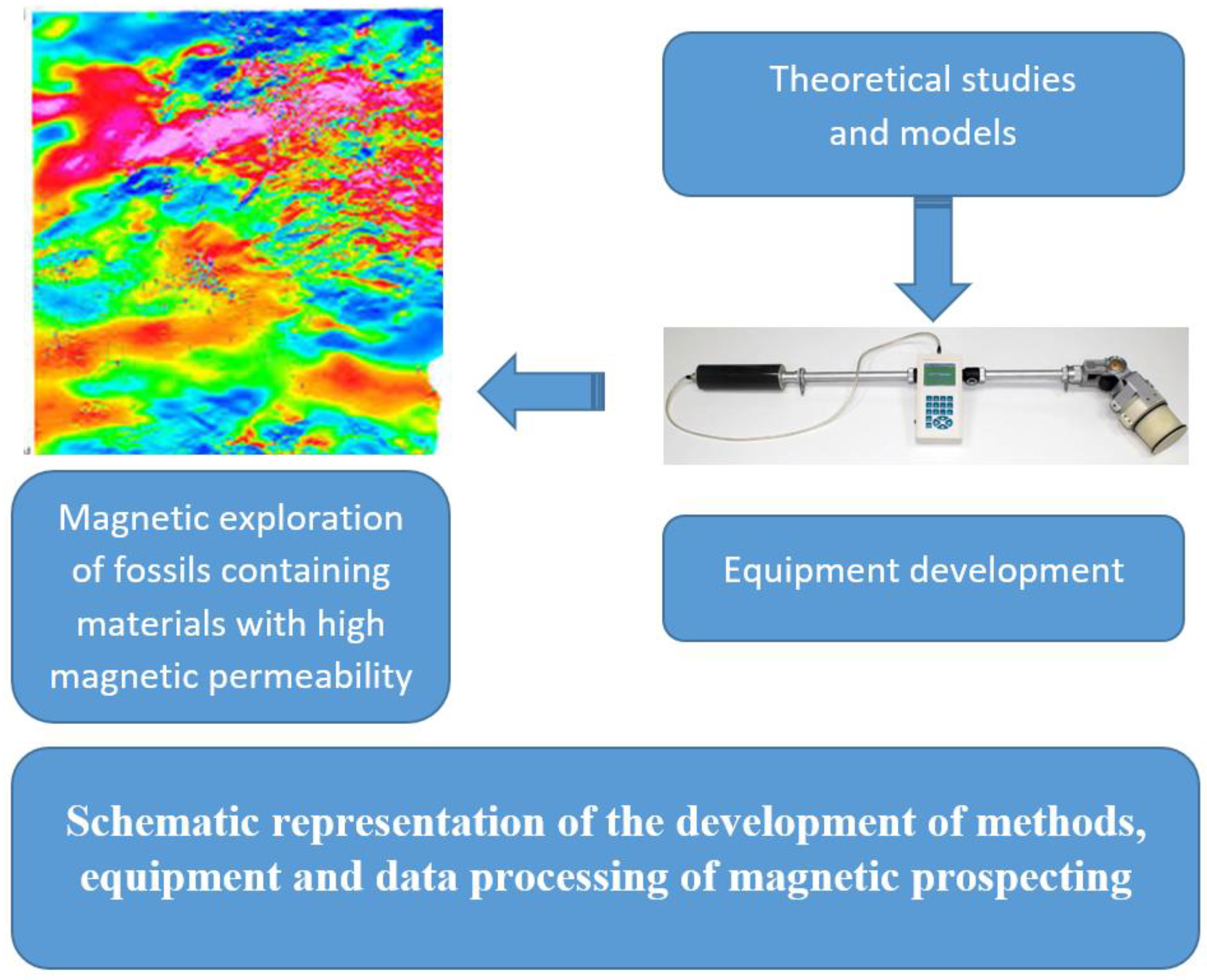
- a schematic representation of the development of methods, equipment, and data processing of magnetic prospecting;
- -
- the goal of this research as the development of a method for magnetic prospecting of, predominantly, fossils containing materials with a high magnetic permeability.
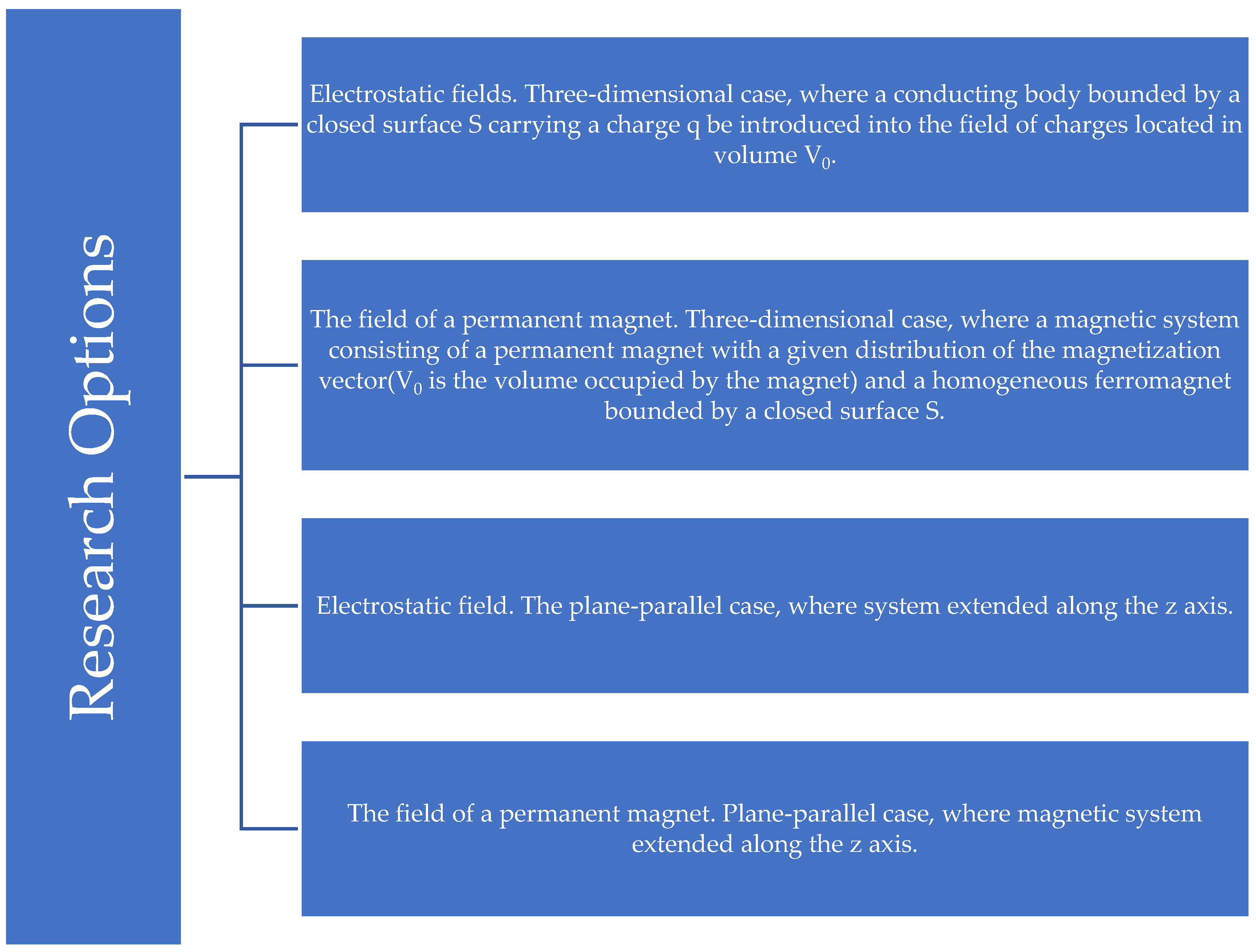
- (A)
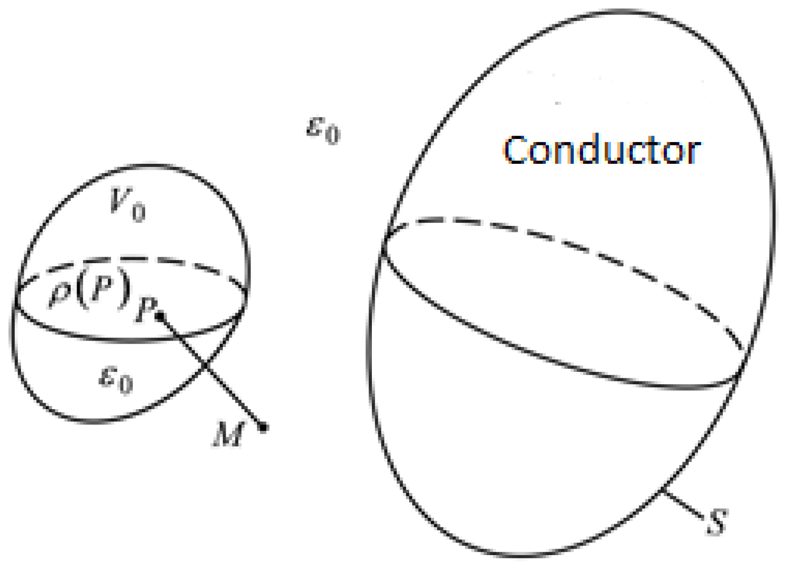
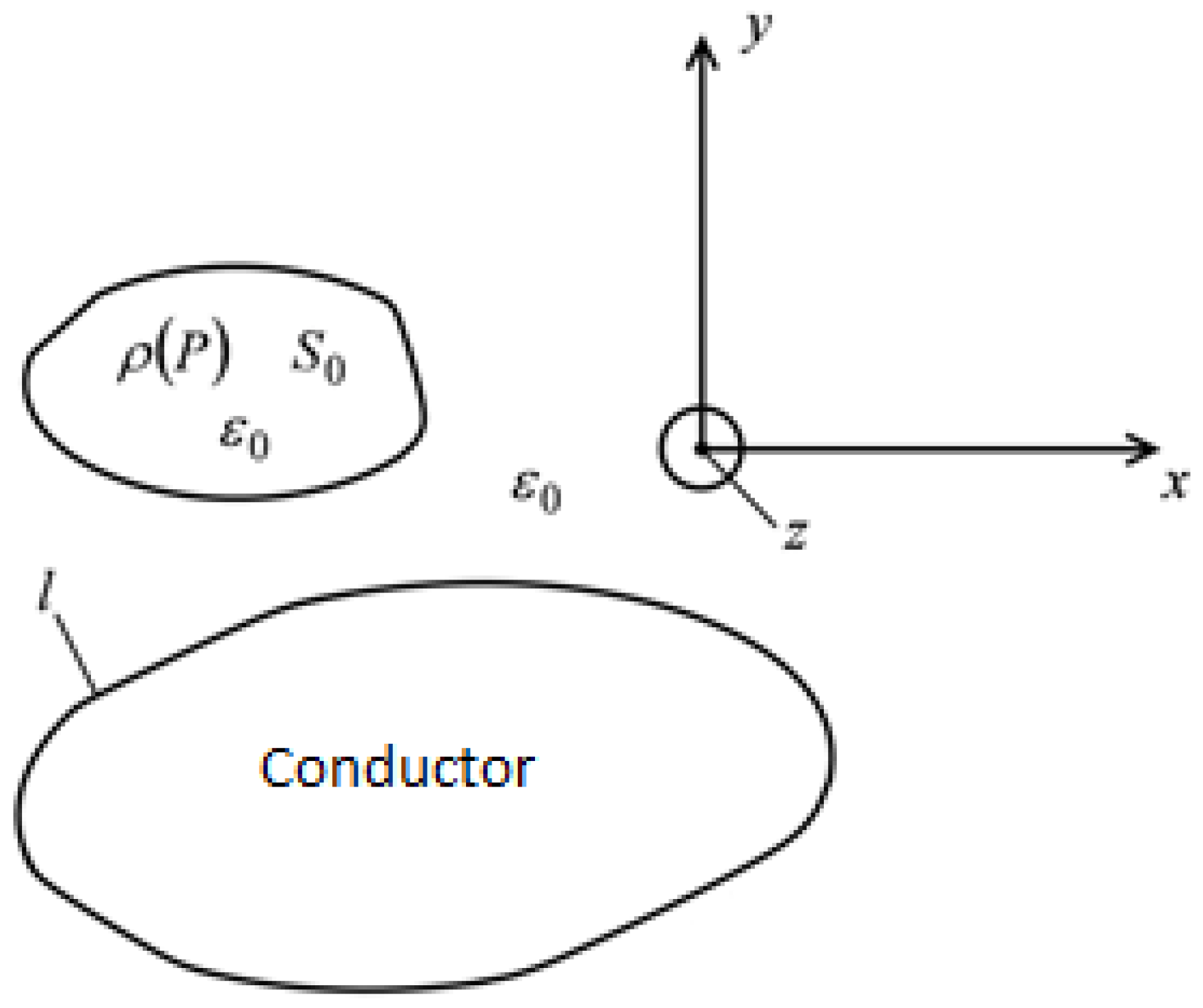
- Electrostatic fields. Three-dimensional case, where a conducting body bounded by a closed surface S carrying a charge q is introduced into the field of charges located in volume V0.
- (B)
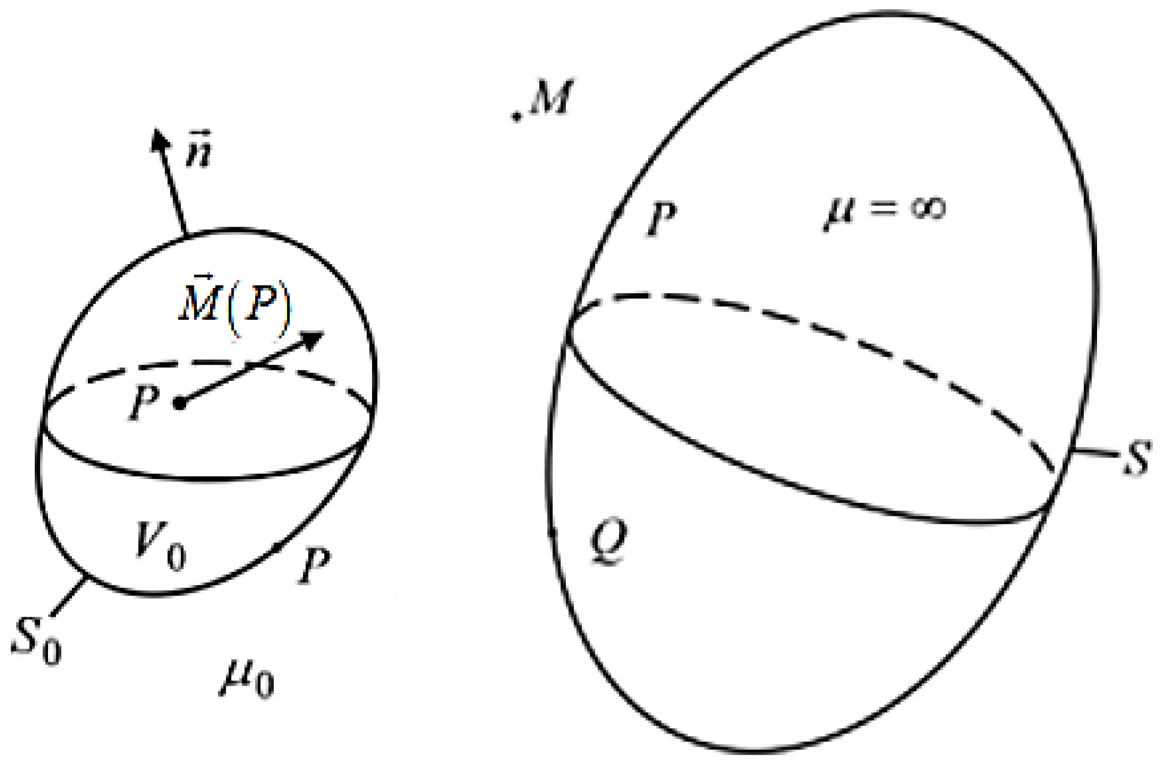
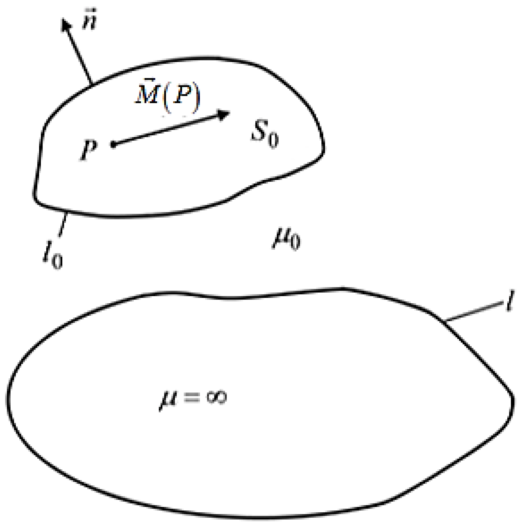
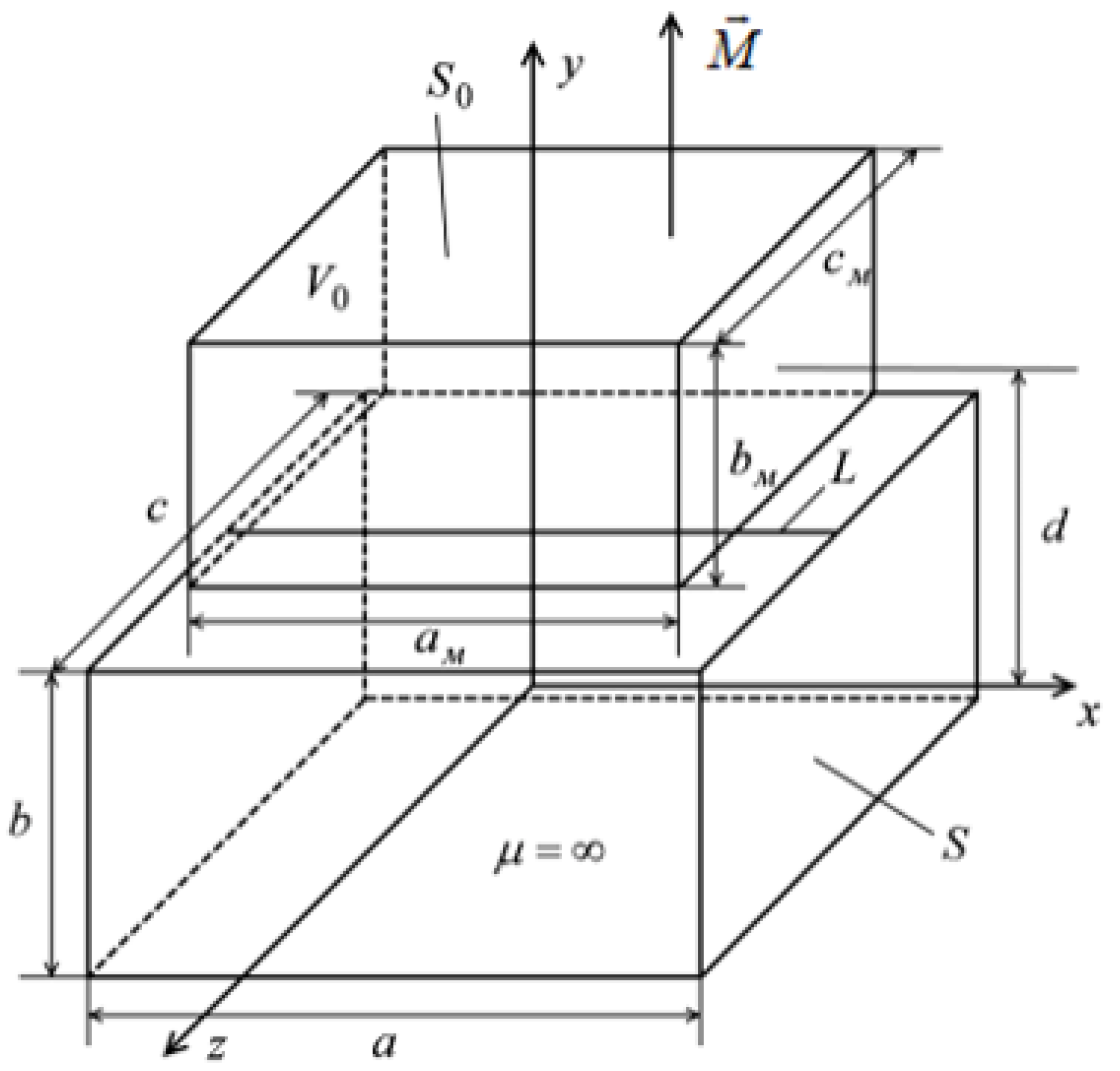
- The field of a permanent magnet. Three-dimensional case, where a magnetic system consists of a permanent magnet with a given distribution of the magnetization vector (V0 is the volume occupied by the magnet) and a homogeneous ferromagnet bounded by a closed surface S.
- (C)
- Electrostatic field. The plane-parallel case, where the system is extended along the z axis.
- (D)
- The field of a permanent magnet. Plane-parallel case, where the magnetic system is extended along the z axis.
2. Materials and Methods
3. Results and Discussion
3.1. The Field of a Permanent Magnet—Three-Dimensional Case
3.2. The Electrostatic Field—The Plane-Parallel Case
3.3. The Field of a Permanent Magnet—The Plane-Parallel Case
3.4. Examples of Calculating Magnetic Fields Using Integral Equations of the First Kind
4. Conclusions
- -
- bring geophysical services to the service market on a new scientific and technical production level;
- -
- reduce the environmental burden on nature by replacing magnetometric measurements with energy-saving, environmentally safe technology;
- -
- ensure the export potential of magnetometric equipment.
Author Contributions
Funding
Institutional Review Board Statement
Informed Consent Statement
Data Availability Statement
Conflicts of Interest
References
- Adelman, R.; Gumerov, N.A.; Duraiswami, R. FMM/GPU-Accelerated Boundary Element Method for Computational Magnetics and Electrostatics. IEEE Trans. Magn. 2017, 53, 1–11. [Google Scholar] [CrossRef]
- Kim, D.H.; Park, I.H.; Park, M.C.; Lee, H.B. 3-D magnetostatic field calculation by a single layer boundary integral equation method using a difference field concept. IEEE Trans. Magn. 2000, 36, 3134–3136. [Google Scholar]
- Andjeli´c, Z.; Ishibashi, K. Double-layer BEM for generic electrostatics. In Proceedings of the 2016 IEEE Conference on Electromagnetic Field Computation (CEFC), Miami, FL, USA, 1 November 2016. [Google Scholar]
- Andjeli´c, Z.; Ishibashi, K.; Barba, P.D. Novel double-layer boundary element method for electrostatic analysis. IEEE Trans. Dielectr. Electr. Insul. 2018, 25, 2198–2205. [Google Scholar] [CrossRef]
- Ishibashi, K.; Yoshioka, T.; Wakao, S.; Takahashi, Y.; Andjelic, Z.; Fujiwara, K. Improvement of unified boundary integral equation method in magnetostatic shielding analysis. IEEE Trans. Magn. 2014, 50, 105–108. [Google Scholar] [CrossRef]
- Ishibashi, K.; Andjelic, Z.; Takahashi, Y.; Takamatsu, T.; Fukuzumi, T.; Wakao, S.; Fujiwara, K.; Ishihara, Y. Magnetic Field Evaluation at Vertex by Boundary Integral Equation Derived from Scalar Potential of Double Layer Charge. IEEE Trans. Magn. 2012, 48, 459–462. [Google Scholar] [CrossRef]
- Ishibashi, K.; Andjelic, Z. Generalized magnetostatic analysis by boundary integral equation derived from scalar potential. IEEE Trans. Magn. 2013, 49, 1533–1536. [Google Scholar] [CrossRef]
- Telegin, A.P.; Klevets, N.I. Calculation of an axisymmetric current coil field with the bounding contour integration method. J. Magn. Magn. Mater. 2004, 277, 257–262. [Google Scholar] [CrossRef]
- Filippov, D.M.; Shuyskyy, A.A. Improving efficiency of the secondary sources method for modeling of the three-dimensional electromagnetic field. Prog. Electromagn. Res. M 2019, 78, 19–27. [Google Scholar]
- Neethu, S.; Nikam, S.; Wankhede, A.K.; Pal, S.; Fernandes, B.G. High speed coreless axial flux permanent magnet motor with printed circuit board winding. In Proceedings of the IEEE Industry Applications Society Annual Meeting, Cincinnati, OH, USA, 1–8 October 2017. [Google Scholar]
- Aydin, M.; Gulec, M. A new coreless axial flux interior permanent magnet synchronous motor with sinusoidal rotor segments. IEEE Trans. Magn. 2016, 52, 1–4. [Google Scholar] [CrossRef]
- Price, G.P.; Batzel, T.D.; Comanescu, M.; Muller, B.A. Design and testing of a permanent magnet axial flux wind power generator. In Proceedings of the 2008 IAJC-IJME International Conference, Music City Sheraton, Nashville, TN, USA, 17–19 November 2008. [Google Scholar]
- Andjelic, Z.; Ishibashi, K.; Lage, C.; Di Barba, P. On a Study of Magnetic Force Evaluation by Double-Layer Approach 2020. IEEE Trans. Magn. 2020, 56, 8956056. [Google Scholar] [CrossRef]
- Ryu, K.; Yoshioka, T.; Wakao, S.; Ishibashi, K.; Fujiwara, K. Magnetostatic Shield Analysis by Double-Layer Charge Formulation Using Difference Field Concept. IEEE Trans. Magn. 2016, 52, 7205604. [Google Scholar] [CrossRef]
- Ryu, K.; Wakao, S.; Takahashi, Y.; Ishibashi, K.; Fujiwara, K. A study on multiply connected domain processing methods in magnetostatic field analysis by boundary integral equations. IEEE Trans. Power Energy 2017, 137, 132–137. [Google Scholar] [CrossRef]
- Filippov, D.M.; Berzhansky, V.N.; Shuyskyy, A.A.; Lugovskoy, N.V. Mathematical modeling and magneto-optical visualization of the electromagnetic field in the neighborhood of defects in conductive materials. CEUR Workshop Proc. 2021, 2914, 324–330. [Google Scholar]
- Filippov, D.M.; Shuyskyy, A.A.; Kazak, A.N. Numerical and experimental analysis of an axial flux electric machine 2020 Proceedings-2020 International Conference on Industrial Engineering, Applications and Manufacturing. ICIEAM 2020, 9112004. [Google Scholar] [CrossRef]
- Ishibashi, K.; Andjelic, Z.; Takahashi, Y.; Fujiwara, K.; Ishihara, Y. Some treatments of fictitious volume charges in nonlinear magnetostatic analysis by BIE. IEEE Trans. Magn. 2012, 48, 463–466. [Google Scholar] [CrossRef]
- Yu, H.; Yuan, J. Improved differential field integral equation method. J. Tsinghua Univ. 2008, 48, 1073–1076. [Google Scholar]
- Hafla, W.; Buchau, A.; Rucker, W.M. Accuracy improvement in nonlinear magnetostatic field computations with integral equation methods and indirect total scalar potential formulations. COMPEL-Int. J. Comput. Math. Electr. Electron. Eng. 2006, 25, 565–571. [Google Scholar] [CrossRef]
- Ishibashi, K.; Andjelic, Z.; Takahashi, Y.; Fujiwara, K.; Ishihara, Y. Magnetostatic analysis by BEM with magnetic double layer as unknown utilizing volume magnetic charge. Int. J. Appl. Electromagn. Mech. 2012, 39, 711–717. [Google Scholar] [CrossRef]
- Charge Ishibashi, K.; Andjelic, Z. Nonlinear magnetostatic BEM formulation using one unknown double layer. COMPEL-Int. J. Comput. Math. Electr. Electron. Eng. 2011, 30, 1870–1884. [Google Scholar] [CrossRef]
- Young, J.C.; Gedney, S.D. A locally corrected Nyström formulation for the magnetostatic volume integral equation. IEEE Trans. Magn. 2011, 47, 2163–2170. [Google Scholar] [CrossRef]
- Young, J.C.; Gedney, S.D.; Adams, R.J. Quasi-mixed-order prism basis functions for nyström-based volume integral equations. IEEE Trans. Magn. 2012, 48, 2560–2566. [Google Scholar] [CrossRef]
- Valve Wang, S.; Cheng, J.; Huang, K.; Zhu, J.; Zhang, W. Research on the Electromagnetic Characteristics of UHV-VSC Converter. In Proceedings of the 2020 7th IEEE International Conference on High Voltage Engineering and Application, ICHVE 2020-Proceedings, Beijing, China, 6–10 September 2020. [Google Scholar]
- Wang, S.; Cheng, J.; Huang, K.; Zhao, L.; Lin, J. Electric field calculation of UHV-VSC valve hall based on instantaneous potential load method. IET Conf. Publ. 2020, 775, 2260–2264. [Google Scholar]
- Yu, H.Y.; He, J.L.; Lee, J.B.; Chang, S.H.; Zou, J. Adaptive Galerkin approach of indirect boundary element method for calculating 3D magnetostatic field with local updating algorithm. In Proceedings of the 2006 12th Biennial IEEE Conference on Electromagnetic Field Computation, Miami, FL, USA, 30 April–2 May 2006. [Google Scholar]
- Filippov, D.M.; Kozik, G.P.; Shuyskyy, A.A.; Kazak, A.N.; Samokhvalov, D.V. A New Algorithm for Numerical Simulation of the Stationary Magnetic Field of Magnetic Systems Based on the Double Layer Concept 2020. In Proceedings of the 2020 IEEE Conference of Russian Young Researchers in Electrical and Electronic Engineering, St. Petersburg and Moscow, Russia, 27–30 January 2020. [Google Scholar]
- Noguchi, S.; Kim, S. Development of numerical simulation method for magnetic separation of magnetic particles. In Proceedings of the 2010 Digests of the 2010 14th Biennial IEEE Conference on Electromagnetic Field Computation, Chicago, IL, USA, 9–12 May 2010. [Google Scholar]
- Banucu, R.; Albert, J.; Scheiblich, C.; Reinauer, V.; Rucker, W.M. Design and optimization of a device with contactless actuation for 4-axis machining 2010. In Proceedings of the 2010 14th Biennial IEEE Conference on Electromagnetic Field Computation, Chicago, IL, USA, 9–12 May 2010. [Google Scholar]
- Hafla, W.; Buchau, A.; Rucker, W.M. Application of fast multipole method to Biot-Savart law computations. In Proceedings of the 6th International Conference on Computational Electromagnetics, Aachen, Germany, 4–6 January 2006. [Google Scholar]
- Zheng, Q.; Zeng, H. Multipole theory analysis of 3D magnetostatic fields. J. Electromagn. Waves Appl. 2006, 20, 389–397. [Google Scholar] [CrossRef]


| Magnetometer Type | Magnetic Sensitive Element | Measured Components |
|---|---|---|
| Optical-mechanical | Permanent magnet | Z, ΔZ |
| Proton | Hydrogen liquid | T, ΔT, ∂T ∂x, ∂T ∂x |
| Overhauser | Hydrogen-containing liquid with the addition of free radicals with unpaired electrons | |
| Quantum | Alkali metal vapors | |
| Ferroprobe | Ferrosonde | X, Y, Z, ΔX, ΔY, ΔZ |
| Cryogenic | Superconducting quantum interferometer | T, ΔT |
| Magnetometer Type | Advantages | Disadvantages |
|---|---|---|
| Optical-mechanical | Able to measure Z, X, Y and H components. | Zero point creep, presence of azimuth correction, temperature drift, low measurement speed, low accuracy. |
| Proton | This magnetometer type is impervious to shaking and vibrations, measurements are practically independent of changes in external conditions (temperature, humidity, pressure), there is no need for precise orientation of the sensor, there is no need to stake out reference networks, zero-point shift is negligible. | Instability and signal loss at high magnetic field gradients. |
| Overhauser | All the benefits of proton magnetometers, plus reduced measurement time, lower uncertainty due to increased signal-to-noise ratio, small sensor size. | Short lifetime of the working substance, the appearance of a systematic error, due to the influence of the microwave unit. |
| Quantum | High measurement speed, high resolution. | The need for orientation of the sensor is present, but with small values: orientation and azimuth errors, temperature drift. Sensitivity to mechanical influences (shock, vibration). |
| Ferroprobe | Able to measure Z, X, Y and H components with high accuracy. | The bulkiness of the equipment, the need to orient the sensor. |
| Cryogenic | High accuracy. | The need to maintain very low temperatures for a superconductor. There are no mass-produced devices. |
| The First Way | The Second Way |
|---|---|
| −2410.29 | −2410.29 |
| −2368.50 | −2368.50 |
| −2354.42 | −2354.42 |
| −2353.95 | −2353.95 |
| −2354.71 | −2354.71 |
| −2354.71 | −2354.71 |
| −2353.95 | −2353.95 |
| −2354.42 | −2354.42 |
| −2368.50 | −2368.50 |
| −2410.29 | −2410.29 |
| The First Way | The Second Way |
|---|---|
| −6020.20 | −6020.20 |
| −6008.95 | −6008.95 |
| −6004.63 | −6004.63 |
| −6004.21 | −6004.21 |
| −6004.25 | −6004.25 |
| −6004.25 | −6004.25 |
| −6004.21 | −6004.21 |
| −6004.63 | −6004.63 |
| −6008.95 | −6008.95 |
| −6020.20 | −6020.20 |
Disclaimer/Publisher’s Note: The statements, opinions and data contained in all publications are solely those of the individual author(s) and contributor(s) and not of MDPI and/or the editor(s). MDPI and/or the editor(s) disclaim responsibility for any injury to people or property resulting from any ideas, methods, instructions or products referred to in the content. |
© 2023 by the authors. Licensee MDPI, Basel, Switzerland. This article is an open access article distributed under the terms and conditions of the Creative Commons Attribution (CC BY) license (https://creativecommons.org/licenses/by/4.0/).
Share and Cite
Plugatar, Y.; Filippov, D.; Chabanov, V.; Kazak, A.; Korzin, V.; Oleinikov, N.; Mayorova, A.; Nekhaychuk, D. Integral Equations of the First Kind for Calculating Electro- and Magnetostatic Fields Perturbed by Conductors and Ferro-Magnets. Inventions 2023, 8, 55. https://doi.org/10.3390/inventions8020055
Plugatar Y, Filippov D, Chabanov V, Kazak A, Korzin V, Oleinikov N, Mayorova A, Nekhaychuk D. Integral Equations of the First Kind for Calculating Electro- and Magnetostatic Fields Perturbed by Conductors and Ferro-Magnets. Inventions. 2023; 8(2):55. https://doi.org/10.3390/inventions8020055
Chicago/Turabian StylePlugatar, Yurij, Dmitriy Filippov, Vladimir Chabanov, Anatoliy Kazak, Vadim Korzin, Nikolay Oleinikov, Angela Mayorova, and Dmitry Nekhaychuk. 2023. "Integral Equations of the First Kind for Calculating Electro- and Magnetostatic Fields Perturbed by Conductors and Ferro-Magnets" Inventions 8, no. 2: 55. https://doi.org/10.3390/inventions8020055