Article

Classification of Different Recycled Rubber-Epoxy Composite Based on Their Hardness Using Laser-Induced Breakdown Spectroscopy (LIBS) with Comparison Machine Learning Algorithms

1
Department of Electrical-Electronics Engineering, Atilim University, Incek Golbasi, Ankara 06830, Turkey
2
Department of Physics & Applied Physics, University of Massachusetts Lowell, Lowell, MA 01854, USA
3
Department of Mechanical Engineering, Atilim University, Incek Golbasi, Ankara 06830, Turkey
4
School of Mechanical and Manufacturing Engineering, ISAE-Supmeca-Paris, Saint Ouen, 93407 Paris, France
*
Authors to whom correspondence should be addressed.
Inventions 2023, 8(2), 54; https://doi.org/10.3390/inventions8020054
Submission received: 25 November 2022 / Revised: 28 December 2022 / Accepted: 9 January 2023 / Published: 8 March 2023
(This article belongs to the Collection Feature Innovation Papers)

Abstract

:
This paper aims toward the successful detection of harmful materials in a substance by integrating machine learning (ML) into laser-induced breakdown spectroscopy (LIBS). LIBS is used to distinguish five different synthetic polymers where eight different heavy material contents are also detected by LIBS. Each material intensity-wavelength graph is obtained and the dataset is constructed for classification by a machine learning (ML) algorithm. Seven popular machine learning algorithms are applied to the dataset which include eight different substances with their wavelength-intensity value. Machine learning algorithms are used to train the dataset, results are discussed and which classification algorithm is appropriate for this dataset is determined.

1. Introduction

Laser-induced breakdown spectroscopy (LIBS) has been applied to the plastic material to classify them [1], especially since plastic toys are very crucial to identify the harmful heavy metals [2]. Carbon-fiber-reinforced polymer (CFRP) has attracted extensive attention in the industrial field due to its advantages of light weight and high hardness [3]. Synthetic polymer samples (2D-structured and multilayer system) have been analyzed using LIBS and the spatial distribution of five different synthetic polymers, namely acrylonitrile butadiene styrene (ABS), polylactic acid (PLA), polyethylene (PE), polyacrylate (PAK) and polyvinylchloride (PVC) have been successfully classified using multivariate statistical approaches (principal component analysis (PCA) and k-means clustering) [4]. For the recycling of polymer e-waste, there is a pressing need for rapid-measurement technologies for the simple identification and classification of these materials [5] and the classification of plastic polymers through laser-induced breakdown spectroscopy [6]. Accuracy influence analysis (AIA), which is classification precision combined with Kernel naïve Bayes, has been used for selecting informative variables of laser-induced breakdown spectroscopy (LIBS) spectra [7]. Laser-induced breakdown spectroscopy spectra analyzed using the k-nearest neighbor and soft independent modeling using class analogy were investigated as methods that can rapidly identify recyclables [8]; ten different types of post-consumer plastics, including five extensively used basic plastics, were analyzed using (LIBS) [9]. The Davies–Bouldin index was employed to determine the initial number of clusters. The average relative standard deviation values of characteristic spectral lines were used as the iterative criterion. With the proposed approach, the classification accuracy for twenty kinds of industrial polymers achieved 99.6% [10]. For the classification of the different plastic samples, some machine learning algorithms were employed for the analysis of the LIBS spectroscopic data, such as the principal component analysis (PCA) and the linear discriminant analysis (LDA) [11]. A novel chemometric strategy was used and was based on a systematic optimization of two factors influencing the discrimination ability: the set of experimental conditions (laser energy, gate delay, and atmosphere) employed for the LIBS analysis and the set of spectral variables used as a basis for the polymer discrimination [12]. LIBS is a powerful tool for plastic investigations in the laboratory with the capacity of simultaneous qualitative and quantitative analysis [13].
Classification of harmful substances needs to be contributed to literature and human health. In the literature, ML applications are newly contribute in LIBS to determine the hazardous substances and classify the ingredient. However, these studies are not related to the appropriate ML method to classify LIBS dataset and make a system but mostly about just training some of ML algorithm and the importance of ML in substances classification. Classification of hazardous chemical substances studies are developed and contribute to literature but dataset are not related with LIBS [5,14]. Therefore, This paper aims to satisfy the requirement for discussion and determination of appropriate ML algorithm for dataset obtained from LIBS.
Classification of different polymer composite materials has been performed based on their hardness. Eight different substances’ intensity-wavelength values are obtained and dataset is occurred. Seven different models is used for train the dataset and results are compared. Fine Gaussian SVM, Fine tree, linear discriminant, Gaussian Naive Bayes, Kernel Naïve Bayes, Quadratic SVM, and KNN are the most valid and high accuracy ML methods in variety of field which are used for training in this paper [15,16,17,18]. For training, MATLAB is used which is preferred programing language for ML applications [19,20]. Models are trained with LIBS dataset, accuracies are compared, discussed and the most accurate model is determined for LIBS dataset.

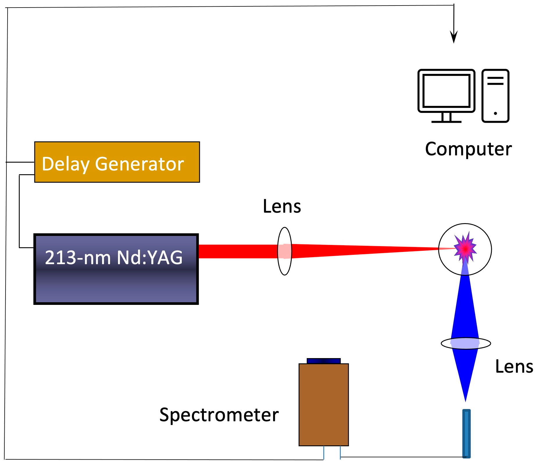
2. Experimental Procedure

Interior mechanism view of LIBS whole system (Applied Spectra, J200 LA) we used is shown in Figure 1. Laser (Quantel) with wavelength of 213 nm, output energy of 20 mJ, pulse width of 10 ns and repetition rate of 100 Hz has been used. Laser beam focused by 10 cm focal length of plano convex lens. Focused beam spot size was 50 μm. A total of 3 different target regions were determined on the same sample surface and these regions were used for spectral measurements. Spectral data were collected via 10 shots to 4 different locations on target-zone surfaces.

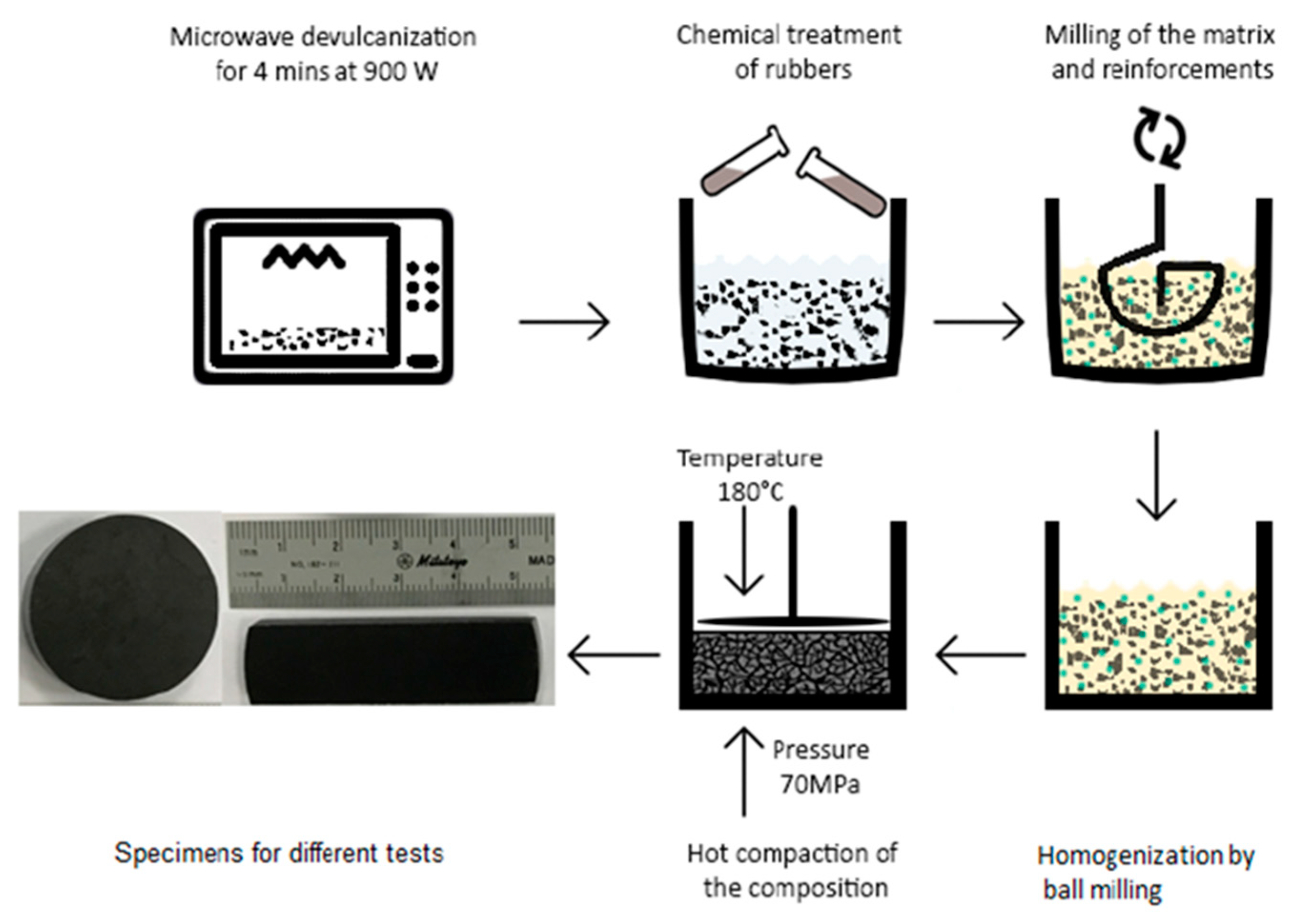
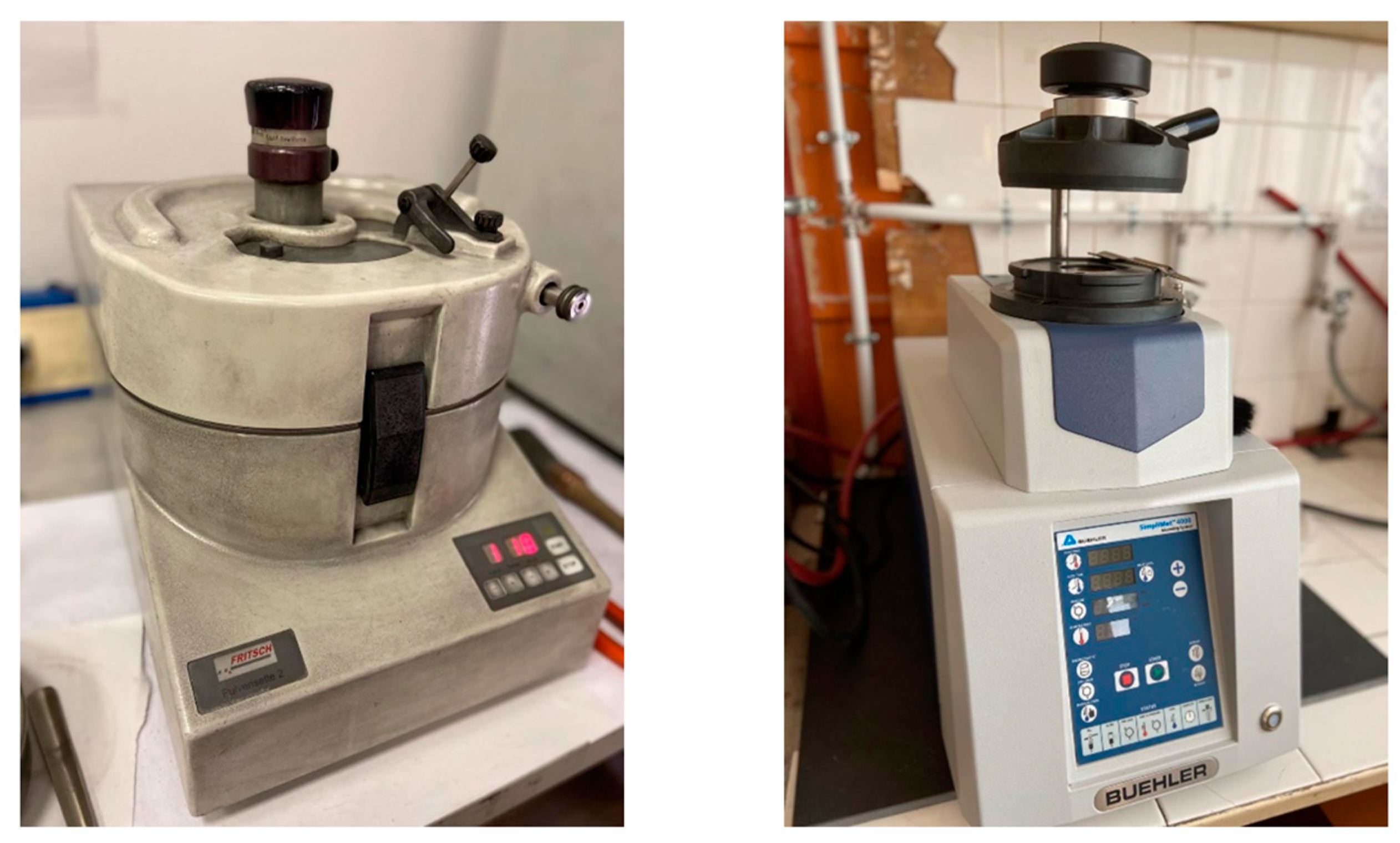
2.1. Sample Preparation

For the manufacturing of recycled rubber-epoxy composite, good quality of bonding between matrix and reinforcements is required, however, recycled rubbers do not carry any free chains to form new bonding with epoxy resin because of the former vulcanization process. In order to improve the interface quality between epoxy and rubber, fresh scrap rubber should be devulcanized. During the devulcanization process, sulfur links are attempted to be broken and other new links are generated, then the flowing capacity and interaction of recycled rubbers with other substances are increased. After determination of the reinforcements with matrix in wt%, a special process is applied to successfully complete the manufacturing of the composites. This process involves silanization of the recycled rubber and devulcanization before blending it with epoxy resin and reinforcement. Chemical treatment followed by devulcanized recycled rubber is mixed with epoxy resin for obtaining a strong chemical-bonding diffusion reinforced with different reinforcement. After blending the mixture, they are milled for 4 h by adding “Zn-Stearate” as a lubricant for homogenous distribution. For manufacturing of the composites, hot compaction is carried out at 180 °C for 20 min under the pressure of 70 MPa; after that, the specimens are produced with a diameter of 50 mm—a similar procedure is given in Figure 2. The equipment used during the process is also presented in Figure 3.

2.2. ML Methods for LIBS

Machine Learning is an artificial intelligence that facilitates the classification of received data. After measured the wavelength values of substances as it is mentioned above, seven different well-known machine learning methods have been tried in order to classify them and determine what ingredients they have. In the literature, it is obvious that the use of artificial intelligence in LIBS is a hot topic for classifying [11,21]. Substance Identification has been made with mostly machine learning which is K- Nearest Neighbours(KNN) [22,23], Support Vector Machine(SVM) [24], Naive Bayes Classification, Principal Component Analysis (PCA), and the Linear Discriminant Analysis (LDA) also applied on spectroscopic data [25]. There is just Deep Belief Network (DBN) which is a deep learning method that has been used on data. The important thing has been seen is that there is no comparison between these methods’ effectiveness on LIBS. In this paper, some of the effective machine learning methods for data classification are compared with each other and the decision on the effective data classification method has been discussed. After classification method is determined, this algorithm will be integrated to the system to collaborate with LIBS. Therefore, the lack in the literature about classification collaboration between LIBS and ML can be satisfied.

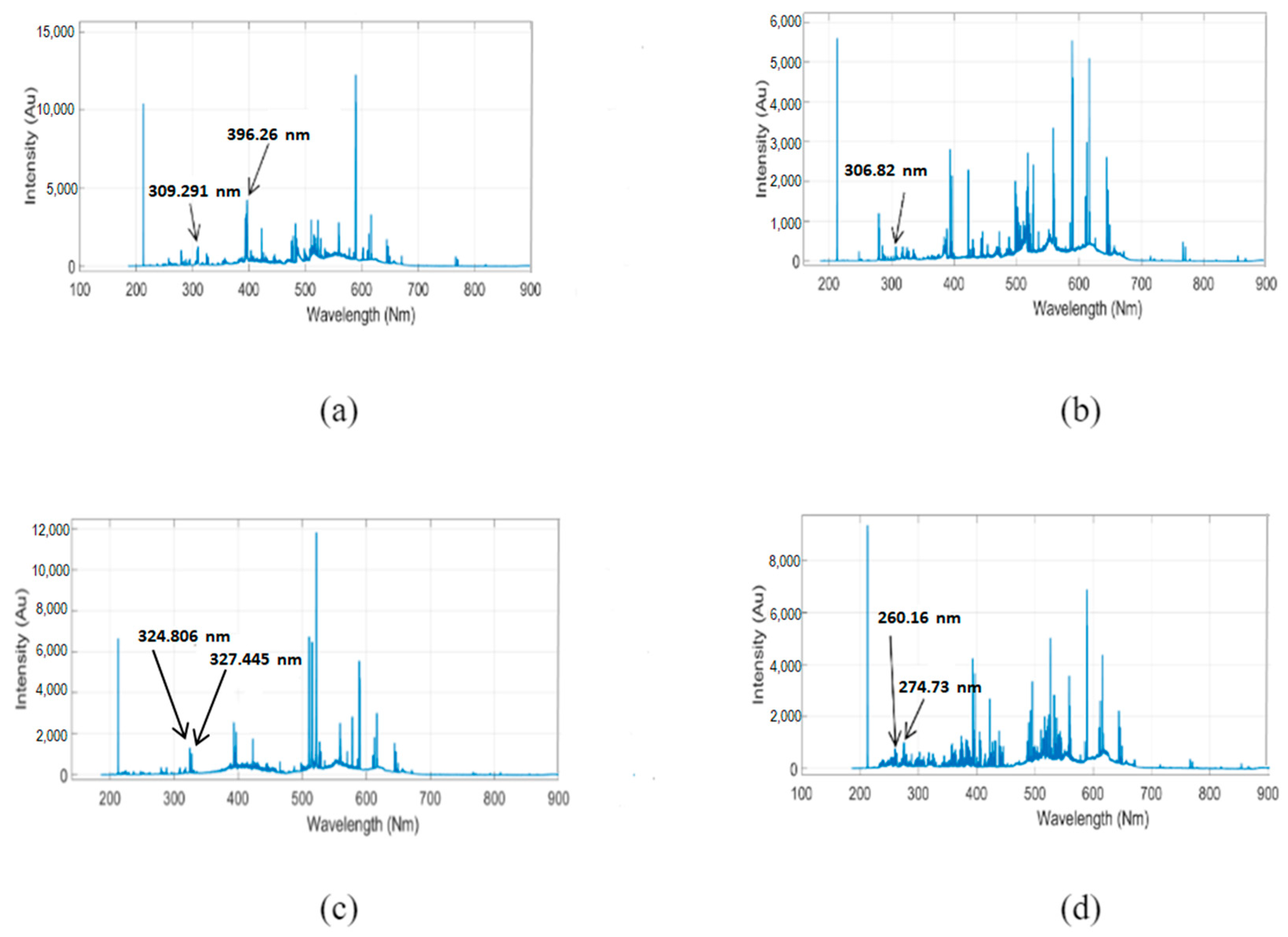
3. Results and Discussion

Dataset obtained from LIBS includes aluminum, copper, bismuth, iron, magnesium, nickel, tin, and zinc wavelength-intensity values. Therefore, we have eight classes for classification. In artificial intelligence (AI) applications, dataset preparation is of crucial importance. If the dataset is not properly prepared and adjusted, it is not important whether the AI model works well or not. Eight different substances in polymer were obtained from the LIBS measurement, which are aluminum (Al), bismuth (Bi), copper (Cu), iron (Fe), magnesium (Mn), nickel (Ni), tin (Sn), zinc (Zn). Forty data were obtained from each substance in the three different locations, so each substance has 120 data in total. Also, wavelengths start from 186.015 to 1048.107 so in the dataset a total of 12286 wavelength values are used. The dimension of the data is 12286x 960 for eight classes. The substance in the polymer has been detected by showing the related wavelength for each substance which is demonstrated below in Figure 4. The original dataset includes negative values which are assumed as noise and eliminated before plotting. Plottings include non-negative values in Figure 4. Also, this big data should not be used directly for obtaining good accuracy because the values of intensity of different classes can be matched or overlapped, therefore mismatch and misclassification inevitably occur. To see the effect of the unadjusted dataset result, this 12,285 × 960-dimension dataset was applied directly to the decision fine tree, which is a supervised machine learning model. The eight classes of substances are orderly determined as aluminum (Al), bismuth (Bi), copper (Cu), iron (Fe), magnesium (Mn), nickel (Ni), tin (Sn), and zinc (Zn); in the algorithm response of the substances determined with numbers, one to eight are orderly. Each substance has 120 data, so 120 responses for each substance were determined; 960 data and responses were used in total. The reason for selecting the fine tree model for classification is that there are so many values, and decision tree accuracy results show whether this dataset is logical or not for training. This fine tree model is used for the unadjusted dataset and the result is obtained and demonstrated, as in Figure 5. Detection with unadjusted dataset is insufficient. This can be interpreted from Figure 5.
Confusion matrices show the accuracy of training, the blue diagonal is interpreted as a true-positive detection of the related class, and the orange boxes belong to the false-negative detection according to the giving response. Total of the true positive over eight gives us the total accuracy of training, so the total accuracy of the unadjusted dataset with the fine tree model is 84.6%. One by one, the confusion matrices can be interpreted as below.
The class one (Al) is detected with 66.7% accuracy as is shown in Figure 5 for the first true positive box, however, some of the data in class one (Al) were detected as class five (Mn) with 26.7%, and some other is classed as six (Ni) with 6.7%, as can be understood from the false-negative orange-colored boxes for the same line.
Another instance, 3.3% of Bi is detected as Ni, 6.7% of the Cu is detected as Ni, and Fe is detected completely true with 100%.
A total of 40% of the Mn is detected as Al and 3.3% of the Mn is detected as Cu, so the total true positive value of the Mn is 56.7%. A total of 3.3% of the Ni is detected as Bismuth and 10% of the Ni is obtained as Sn, so the total accuracy of the Ni is 86.7%. 6.7% of the Sn is founded as Cu and 16.7% of the Sn is identified as Ni, therefore the total trueness of the Sn is 76.7% while Zn is detected as completely true-positive with 100%. The overall accuracy of the model with this non-adjusted dataset is obtained with the mean of true-positive percentages of the classes which have been founded being 84.6%. Other confusion matrices are interpreted as mentioned above, and the most accurate ML algorithm for this dataset is determined for using in automatic classification with LIBS.
As it is mentioned above, 120 responses were determined for each category separately, so Y is defined as 960 responses for eight classes. This gives us the accuracy and errors for the total and for each class. During the model-making classification, these defined response data are taken as a basis for true classification. The classification graph of the response data is shown in Figure 6.
A data adjustment was made to eliminate false detection caused by using the non-adjusted dataset. Every substance has its own intensity value in a specific wavelength interval, as it is shown in Figure 4. For instance, Al has its peak value at 309.291 nm and 396.29 nm, while Bi has it at 306.82 nm. Cu has been detected at 324.806 nm and 327.445 nm, Fe at 324.806 nm and 327.447 nm, while Mn has three different intensity values at 257.619 nm, 279.585 nm, and 294.985 nm. Ni has a peak intensity at 300.248 nm. Sn is detected at 284.08 nm and 326.303 nm, while Zn has a peak value at 213.959 nm. Dataset adjusted in the direction of these peak values for each class. By focusing on its own peak values for each substance, the new dataset was created based on the circumference of the wavelength that belonged to the peak values.
Seven different models have been trained and compared: the fine Gaussian SVM, fine tree, linear discriminant, Gaussian Naïve Bayes, Kernel Naïve Bayes, Quadratic SVM, and KNN on the adjusted dataset. MATLAB is used for applying ML algorithms to the dataset which is also widely used in ML studies. The model which gives the best result is tested and demonstrated also.
The fine tree model has been trained again for the new adjusted dataset. This model compares the similarities between classes and focuses on reducing the error while comparing [26].
The fine-tree-model accuracy is obtained as 97.9% with adjusted dataset as it is demonstrated in Figure 7. It is clearly evident that data adjustment plays a critical role in the training process. For this dataset, Zn and Ni are completely detected and other classes have 3.1% error in total; Cu mostly gives the false negative by having percentages in two classes.
The second trained model is the fine Gaussian SVM. It can map data to an infinite dimensionality, so it is suitable for training high-dimensional datasets [27]. Formula of the fine Gaussian SVM is shown below.
G X J   , X k = e x p ( X j X k 2   )
it calculates the similarities between Xj and Xk by measuring the Euclidean distance between Xj and Xk. According to formula one, the model is trained, and the accuracy of the fine Gaussian SVM model is obtained as 86.5%, the result being quite worse since the SVM has a linear classifier and such a complex dataset needs to be trained with nonlinear solvers. Confusion matrices are shown below.
This model truly detected Cu with 100% and other classes have an error, however, the accuracy is over the 75% and the lowest value also belongs to Al as it is demonstrated in Figure 8.
The linear discriminant is another method for classification. It uses dimension reduction to increase the distance between the mean of classes and it is also appropriate for classifying multi-classes. The linear discriminant model accuracy is obtained as 97.5% as it is shown in Figure 9. In addition to being linear, the accuracy rate is higher than the SVM because it maximizes the distance between the classes and the estimator discriminates the classes from each other by estimating the distinct presence for each class. This model classifies four classes as completely true. The worse prediction is 90%, which is Fe. Generally, a false prediction is made for the Al substance.
The Gaussian Naïve Bayes is another machine learning model which uses the Gaussian probability distribution function. This is a simpler method than other methods because it uses only the mean and standard deviation of the data to generate the new estimated data.
The Gaussian Naïve Bayes classifier gives 98.125% accuracy and predicts five classes as truly, which are Al, Fe, Ni, Sn, Zn. The worse classification is bismuth, and the worse percentage is 93.3% (Figure 10). However, the classifier gives better results than the previous models.
The whole Naïve Bayes classifiers are highly effective and quick to classify. The basis of this algorithm is probability, so it assumes an independent feature of a class that differentiates the estimated from other classes. The Kernel function used in the Naïve Bayes model is named as Kernel Naïve Bayes. It is a successful model for target estimation, since it uses the mean of training samples located around the target and reaches the target value by updating the weight function according to these mean of training samples.
The Kernel Naïve Bayes model accuracy is obtained as 99.0% in Figure 11. The blue line shows the true predictions percentages. According to these confusion matrices, five classes were detected as fully true-positive: Al, Cu, Fe, Ni, Sn. Total prediction percentages over total class gives us the accuracy. The worse percentage is 93.3%. This model gives better result than the previous models. The best result is obtained from this model due to its nonlinear solver and estimation method mentioned above. Such multi-classes, a complex and overlapping dataset, can only be predicted with such a non-linear model.
One of the nonlinear algorithms of the support vector machine is the quadratic SVM. This model uses the same technique with the SVM but the QSVM assumes the classification line with hyper-planes, hyper-spheres, hyper-ellipsoids, hyper-paraboloids, and hyper-hyperboloids of various types.
The quadratic SVM accuracy is obtained as 97.3% in Figure 12. Four classes, Al, Cu, Sn, and Zn are classified as true positive with 100%. It gives better results than the SVM, so the nonlinear model of support vector machine is superior to the standard SVM for this type of dataset.
The distance of the point to be estimated from other points is calculated. The Minkowski distance calculation function is used for this calculation [28]. Nonlinear fitting has been used for this algorithm, but sometimes linear KNN also can be used. In the direction of regression, accuracy is obtained as 97.9% in Figure 13. Four classes are detected as completely true, and the lowest value belongs to Fe with 90%. Even though its total accuracy is high, class accuracy is low as in the QSVM.
In the direction of these comparisons and interpretations, the Kernel Naïve Bayes gives the best result with an accuracy of 99.0%; the Kernel Naïve Bayes was studied for LIBS in the literature as it is mentioned in the introduction part, so it is proved that this model gives high accuracy for the LIBS dataset [7]. Secondly, the Gauss Naïve Bayes gives the best result with an accuracy of 98.125%. Moreover, other nonlinear models are nearly the same, as in the linear models SVM and linear-regression models, however, linear regression gives a better result, which is quite similar to nonlinear models. The classification graph of eight substances with the Kernel Naïve Bayes model is shown below.
The prediction of the eight classes is demonstrated in Figure 14; classified data with the Kernel Naïve Bayes model have been shown. As it can be seen in Figure 14, the orange points out of line mean the classified data have a deviation from other classes; however, it is known that the classification accuracy is 99.0% and has 1% deviation for this model, so it can be easily interpreted that eight substances’ data are highly placed in the predicted class.

4. Conclusions

This paper represents the classification of different polymer composite materials and performed based on their hardness. The hardness-determination process of polymers was made first, then the wavelength-intensity graph of polymers was obtained from LIBS for eight classes, which are aluminium, copper, bismuth, iron, magnesium, nickel, tin, and zinc.
These substances (reinforcements) were classified with seven different models and their comparisons have been shown. Firstly, the data adjustment has been made to increase the accuracy, and no adjusted data effect has been conceived. In light of the training of seven different model and their data adjusting eight classes were trained with seven different model with adjusted dataset. Nearly the same prediction of the response (Figure 6) has been obtained in the classification of graph of Kernel Naïve Bayes model.(Figure 14). Since the Kernel Naïve Bayes’s weights function uses non-parametric estimation techniques, it gives the best result with an accuracy percentage of 99.0. As a result, this model is the most appropriate model for this dataset to use in LIBS to detect substance ingredients automatically.

Author Contributions

Conceptualization, O.A.; Methodology, V.S.Y. and E.B.; Software, V.S.Y.; Validation, K.E.E., O.A. and E.B.; Formal analysis, K.E.E. and E.B.; Investigation, K.E.E.; Data curation, V.S.Y.; Writing—original draft, K.E.E.; Writing—review & editing, O.A. and E.B. All authors have read and agreed to the published version of the manuscript.

Funding

This research received no external funding.

Data Availability Statement

Not applicable.

Conflicts of Interest

The authors declare no conflict of interest.

References

  1. Li, K.; Qiu, C.; Tian, D.; Yang, G.; Li, Y.; Han, X. Laser-Induced Breakdown Spectroscopy for Plastic Classification. Spectrosc. Spectr. Anal. 2017, 37, 3600–3605. [Google Scholar]
  2. Godoi, Q.; Leme, F.O.; Trevizan, L.C.; Pereira Filho, E.R.; Rufini, I.A.; Santos, D., Jr.; Krug, F.J. Laser-induced breakdown spectroscopy and chemometrics for classification of toys relying on toxic elements. Spectrochim. Acta Part B At. Spectrosc. 2011, 66, 138–143. [Google Scholar] [CrossRef]
  3. Wang, W.; Sun, L.; Lu, Y.; Qi, L.; Wang, W.; Qiao, H. Laser induced breakdown spectroscopy online monitoring of laser cleaning quality on carbon fiber reinforced plastic. Opt. Laser Technol. 2022, 145, 107481. [Google Scholar] [CrossRef]
  4. Brunnbauer, L.; Larisegger, S.; Lohninger, H.; Nelhiebel, M.; Limbeck, A. Spatially resolved polymer classification using laser induced breakdown spectroscopy (LIBS) and multivariate statistics. Talanta 2020, 209, 120572. [Google Scholar] [CrossRef]
  5. Costa, V.C.; Aquino, F.W.B.; Paranhos, C.M.; Pereira-Filho, E.R. Identification and classification of polymer e-waste using laser-induced breakdown spectroscopy (LIBS) and chemometric tools. Polym. Test. 2017, 59, 390–395. [Google Scholar] [CrossRef]
  6. Anzano, J.; Bonilla, B.; Montull-Ibor, B.; Lasheras, R.-J.; Casas-Gonzalez, J. Classifications of Plastic Polymers based on Spectral Data Analysis with leaser induced Breakdown Spectroscopy. J. Polym. Eng. 2010, 30, 177–188. [Google Scholar] [CrossRef]
  7. Xu, L.; Liang, L.; Zhang, T.; Tang, H.; Wang, K.; Li, H. A method of improving classification precision based on model population analysis of steel material for laser-induced breakdown spectroscopy. Anal. Methods 2014, 6, 8374–8379. [Google Scholar] [CrossRef]
  8. Jull, H.; Bier, J.; Künnemeyer, R.; Schaare, P. Classification of recyclables using laser-induced breakdown spectroscopy for waste management. Spectrosc. Lett. 2018, 51, 257–265. [Google Scholar] [CrossRef]
  9. Junjuri, R.; Zhang, C.; Barman, I.; Gundawar, M.K. Identification of post-consumer plastics using laser-induced breakdown spectroscopy. Polym. Test. 2019, 76, 101–108. [Google Scholar] [CrossRef]
  10. Guo, Y.; Tang, Y.; Du, Y.; Tang, S.; Guo, L.; Li, X.; Lu, Y.; Zeng, X. Cluster analysis of polymers using laser-induced breakdown spectroscopy with K-means. Plasma Sci. Technol. 2018, 20, 065505. [Google Scholar] [CrossRef] [Green Version]
  11. Stefas, D.; Gyftokostas, N.; Bellou, E.; Couris, S. Laser-Induced Breakdown Spectroscopy Assisted by Machine Learning for Plastics/Polymers Identification. Atoms 2019, 7, 79. [Google Scholar] [CrossRef] [Green Version]
  12. Gajarska, Z.; Brunnbauer, L.; Lohninger, H.; Limbeck, A. Identification of 20 polymer types by means of laser-induced breakdown spectroscopy (LIBS) and chemometrics. Anal. Bioanal. Chem. 2021, 413, 6581–6594. [Google Scholar] [CrossRef]
  13. Zeng, Q.; Sirven, J.-B.; Gabriel, J.-C.P.; Tay, C.Y.; Lee, J.-M. Laser induced breakdown spectroscopy for plastic analysis. TrAC Trends Anal. Chem. 2021, 140, 116280. [Google Scholar] [CrossRef]
  14. Tang, Y.; Guo, Y.; Sun, Q.; Tang, S.; Li, J.; Guo, L.; Duan, J. Industrial polymers classification using laser-induced breakdown spectroscopy combined with self-organizing maps and K-means algorithm. Optik 2018, 165, 179–185. [Google Scholar] [CrossRef]
  15. Dastjerdi, M.V.; Mousavi, S.J.; Soltanolkotabi, M.; Zadeh, A.N. Identification and Sorting of PVC Polymer in Recycling Process by Laser-Induced Breakdown Spectroscopy (LIBS) Combined with Support Vector Machine (SVM) Model. Iran. J. Sci. Technol. Trans. A Sci. 2018, 42, 959–965. [Google Scholar] [CrossRef]
  16. Hussain, L. Detecting epileptic seizure with different feature extracting strategies using robust machine learning classification techniques by applying advance parameter optimization approach. Cogn. Neurodyn. 2018, 12, 271–294. [Google Scholar] [CrossRef]
  17. Wahab, A.H.B.A.; Zahari, R.; Lim, T.H. Detecting diseases in Chilli Plants Using K-Means Segmented Support Vector Machine. In Proceedings of the 2019 3rd International Conference on Imaging, Signal Processing and Communication (ICISPC), Singapore, 27–29 July 2019; IEEE: Piscataway, NJ, USA, 2019; pp. 57–61. [Google Scholar] [CrossRef]
  18. Joshi, S.; Joshi, F. Human Emotion Classification based on EEG Signals Using Recurrent Neural Network And KNN. arXiv 2022, arXiv:2205.08419. [Google Scholar]
  19. Santhiya, R.; GeethaPriya, C. Machine Learning Techniques for Intelligent Transportation Systems-An overview. In Proceedings of the 2021 12th International Conference on Computing Communication and Networking Technologies (ICCCNT), Kharagpur, India, 6–8 July 2021; IEEE: Piscataway, NJ, USA, 2021; pp. 1–7. [Google Scholar]
  20. Rathore, D.S.; Ram, B.; Pal, B.L.; Malviya, S. Analysis of classification algorithms for insect detection using MATLAB. In Proceedings of the 2nd International Conference on Advanced Computing and Software Engineering (ICACSE), Sultanpur, India, 8–9 February 2019. [Google Scholar]
  21. Zhang, D.; Zhang, H.; Zhao, Y.; Chen, Y.; Ke, C.; Xu, T.; He, Y. A brief review of new data analysis methods of laser-induced breakdown spectroscopy: Machine learning. Appl. Spectrosc. Rev. 2022, 57, 89–111. [Google Scholar] [CrossRef]
  22. Dong, R.; Wang, J.; Weng, S.; Yuan, H.; Yang, L. Field determination of hazardous chemicals in public security by using a hand-held Raman spectrometer and a deep architecture-search network. Spectrochim. Acta Part A Mol. Biomol. Spectrosc. 2021, 258, 119871. [Google Scholar] [CrossRef] [PubMed]
  23. Niu, C.; Cheng, X.; Zhang, T.; Wang, X.; He, B.; Zhang, W.; Feng, Y.; Bai, J.; Li, H. Novel Method Based on Hollow Laser Trapping-LIBS-Machine Learning for Simultaneous Quantitative Analysis of Multiple Metal Elements in a Single Microsized Particle in Air. Anal. Chem. 2021, 93, 2281–2290. [Google Scholar] [CrossRef]
  24. Chen, T.; Zhang, T.; Li, H. Applications of laser-induced breakdown spectroscopy (LIBS) combined with machine learning in geochemical and environmental resources exploration. TrAC Trends Anal. Chem. 2020, 133, 116113. [Google Scholar] [CrossRef]
  25. Syazwani, R.W.N.; Asraf, H.M.; Amin, M.M.S.; Dalila, K.N. Automated image identification, detection and fruit counting of top-view pineapple crown using machine learning. Alex. Eng. J. 2022, 61, 1265–1276. [Google Scholar] [CrossRef]
  26. Seyidbayli, C.; Salhi, F.; Akdogan, E. Comparison of machine learning algorithms for EMG signal classification. Period. Eng. Nat. Sci. (PEN) 2020, 8, 1165–1176. [Google Scholar]
  27. Syed, S.A.; Rashid, M.; Hussain, S.; Imtiaz, A.; Abid, H.; Zahid, H. Inter classifier comparison to detect voice pathologies. Math. Biosci. Eng. 2021, 18, 2258–2273. [Google Scholar] [CrossRef] [PubMed]
  28. Arslan, H.; Orhan, E.R. A Comparative Study on COVID-19 Prediction Using Deep Learning and Machine Learning Algorithms: A Case Study on Performance Analysis. Sak. Univ. J. Comput. Inf. Sci. 2022, 5, 71–83. [Google Scholar] [CrossRef]
Figure 1. Depiction of the LIBS system used in this study.
Inventions 08 00054 g001
Figure 2. Manufacturing steps of liquid epoxy-based recycled EPDM-modified composites.
Inventions 08 00054 g002
Figure 3. Milling (left) and hot compaction (right) of the mixture.
Inventions 08 00054 g003
Figure 4. Detected substances of LIBS data obtained from measurement; (a) Al, (b) Bi, (c) Cu, (d) Fe, (e) Mn, (f) Ni, (g) Sn, (h) Zn.
Inventions 08 00054 g004aInventions 08 00054 g004b
Figure 5. Classification of non-adjusted dataset with fine tree machine-learning-model confusion matrices.
Inventions 08 00054 g005
Figure 6. Demonstration of response of the prediction.
Inventions 08 00054 g006
Figure 7. Fine-tree-model confusion matrices.
Inventions 08 00054 g007
Figure 8. Fine Gaussian SVM model confusion matrices.
Inventions 08 00054 g008
Figure 9. Linear-discriminant-model confusion matrices.
Inventions 08 00054 g009
Figure 10. Gaussian-Naïve-Bayes-model confusion matrices.
Inventions 08 00054 g010
Figure 11. Kernel-Naïve-Bayes-model confusion matrices.
Inventions 08 00054 g011
Figure 12. Quadratic SVM confusion matrices.
Inventions 08 00054 g012
Figure 13. KNN model confusion matrices.
Inventions 08 00054 g013
Figure 14. The classification of graph of Kernel Naïve Bayes model.
Inventions 08 00054 g014
Disclaimer/Publisher’s Note: The statements, opinions and data contained in all publications are solely those of the individual author(s) and contributor(s) and not of MDPI and/or the editor(s). MDPI and/or the editor(s) disclaim responsibility for any injury to people or property resulting from any ideas, methods, instructions or products referred to in the content.

