Execution Time Decrease for Controllers Based on Adaptive Particle Swarm Optimization

Abstract

Execution time is an important topic when using metaheuristic-based optimization algorithms within control structures. This is the case with Receding Horizon Control, whose controller makes predictions based on a metaheuristic algorithm. Because the closed loop’s main time constraint is that the controller’s run time must be smaller than the sampling period, this paper joins the authors’ previous work in investigating decreasing execution time. In this context, good results have been obtained by introducing the “reference control profile” concept that leads to the idea of adapting the control variables’ domains for each sampling period. This paper continues to address this concept, which is adjusted to harmonize with the Particle Swarm Optimization algorithm. Moreover, besides adapting the control variables’ domains, the proposed controller’s algorithm tunes these domains to avoid losing convergence. A simulation study validates the new techniques using a nontrivial process model and considering three modes in which the controller works. The results showed that the proposed techniques have practical relevance and significantly decrease execution time.

1. Introduction

Control engineering applications (see [1,2,3,4,5]) frequently use metaheuristic algorithms (see [6,7,8]) because of their robustness and the different process types they can deal with. The controlled processes may include nonlinearities or imprecise, incomplete, and uncertain knowledge. The main drawback of using them is the large controller’s computational effort, which could involve a large execution time that must be prevented from surpassing the sampling period. This is a time constraint mandatory for the controller’s implementation. In this context, decreasing metaheuristic algorithm execution time is an important topic for control applications.

This paper considers the optimal control applications using a well-known control structure, Receding Horizon Control (RHC) (see [9,10]), which includes a metaheuristic algorithm (MA). It is a continuation of our previous work, where different optimal control problems (OCPs) have been solved using RHC (see [11,12,13]). Some MAs are used, and some methods for decreasing execution time are proposed.

RHC has retained our attention due to several characteristics:

• RHC is a control structure that uses a process model (PM).
• Its controller computes optimal control sequences over a prediction horizon based on the PM (see [10,13,14]) at each sampling period.
• A metaheuristic, such as Particle Swarm Optimization Algorithm or Evolutionary Algorithm, can be integrated by the controller to make quasi-optimal predictions (see [13,15,16,17]).

These characteristics constitute the scientific context of the previous works that this paper is a continuation of. This paper concerns the works that have been devoted to the execution time decrease. In each control step, a metaheuristic algorithm searches for the best prediction over the current prediction horizon.

Our work does not concern the computation complexity of a problem [18,19], but it is devoted to the execution time decrease for the proposed predictors. The proof is made using an empirical “a posteriori” analysis. Papers using PSO algorithms for different applications have proposed methods for decreasing execution time. For example, the paper [20] addresses the time complexity of the PSO algorithm. A simple analysis underlines that the number of computations is the sum of those required by the cost function calculation and those involved by the position and velocity update. Both are directly proportional to the number of iterations. To decrease the execution time of PSO algorithms many papers have a general approach, which is to increase the convergence speed through the inertia weight adaptation (see [21]) or the updating of the hyperparameter coefficients [22].

The key principle that can lead to execution time reduction is “the larger the search space, the bigger the execution time”. A practical method to reduce the search space is to shrink the control output domains (from the controller’s point of view, or equivalently, control input domains for the controlled process). Usually, the control variables take values inside the known technological limits. Our general approach exploits additional information concerning the control output domains, allowing us to shrink them. In this way, some non-useful subdomains are cut off without affecting the algorithm convergence.

In this context, a soft sensor presented in [23], called in each sampling period, gives information useful for shrinking the intervals where the control outputs take values. The proposed method devoted to a special process is based on a physical parameter measurement.

Paper [24] has proposed a module integrated into the controller to replace the soft sensor. This module estimates the future process states using the PM for a short time horizon. The proposed method needs a “state quality criterion” that filters the control output values. The simulation programs have used evolutionary algorithms (EAs).

Having the same objective, the paper [25] has proposed a discretization method that can be applied when the metaheuristic is an EA. Regardless of prediction horizon length, the control sequence encoding uses the same number of genes. The execution time decreases because the discretization step increase has a small influence on computation accuracy.

A new method to reduce execution time is proposed in [26], where the metaheuristic used in simulations is also based on EAs. A quasi-optimal control profile, defined as a sequence of control values, is determined offline before controlling the real system. The main idea is that the control outputs should take values inside a specified control profile’s neighborhood. The simulation results prove that the execution time is significantly diminished.

Particle swarm optimization algorithms have been used to solve different OCPs [4,13,23,27,28], especially integrated into the RHC structure. This metaheuristic employed in the same context can also lead to effective methods that reduce execution time, which is the target of our work presented in this paper.

Our paper continues the research work presented in [26] and has the same approach concerning the execution time decrease. The basic characteristic adopted by the two papers are the following:

• The OCP’s solution is a closed-loop solution, not a sequence of control output values. The entire approach may be described by the 4-tuple RHC–Controller–Predictor–Metaheuristic.
• The closed-loop has an RHC structure, which includes a PM.
• An optimization module uses a metaheuristic algorithm to make predictions.
• The metaheuristics use a quasi-optimal control profile determined offline before controlling the real system. The control structure employs this control profile to shrink the control ranges, wherein the control outputs take values.
• The controller adapts the control output ranges at each sampling period, and calls the prediction module (Predictor) so that the Predictor will be more efficient in finding the best prediction.
• The present work’s novelties beyond those of the paper [26] are mentioned hereafter.
• Instead of using EA as a metaheuristic, the prediction module is based on an adaptive variant of the Hybrid topology particle swarm optimization [29,30], referred to as Adaptive Particle Swarm Optimization Algorithm (APSOA).
• The controller sets the control ranges resulting from the control profile and adapts them to the prediction moment. In addition, the Predictor tunes the control ranges; i.e., adjusts the intervals’ length wherein the control outputs take values. The tuning aims to progressively increase the control ranges’ size, not to lose convergence of the APSOA when control ranges are too small.

Our work is validated through a simulation study devoted to a specific OCP, also mentioned in the paper [26]. The latter has another topic and does not deal with execution time decrease. We are reconsidering this OCP to set out a nontrivial case study to which we will apply our execution time-decreasing method. The PM is a nonlinear system that originates in a distributed-parameter system, from which it inherits a certain complexity.

Besides the controller proposed in [23], the present work proposes two new controllers. The first one uses a predefined CP and adapts control ranges to each sampling period before calling the Predictor. The second one has the same tasks, but its Predictor can also make the tunning of control ranges in conjunction with the APSOA.

Section 2 and Section 3 briefly recall the notion of Receding Horizon Control using a MA and the Control Profile approach such that the paper preserves its self-content character. The specific controller structure proposed in our work, using predictions based on the APSOA, is described in Section 4.

After giving the algorithms of the new controllers in Section 5, we conducted simulation series for the old and new controllers and made a comparative analysis in Section 6. The simulation results entitle us to conclude that the proposed method significantly diminishes execution time.

2. Control Horizon Discretizationand Predictions

This section contains some preparatives for using the RHC structure (see [11,12,13,23,26]). The controller’s optimal predictions can be found using metaheuristics, such as Adaptive Particle Swarm Optimization.

When we use metaheuristic algorithms to solve OCPs, we must discretize the control horizon $[0 t_{final}]$ and control outputs,

$$U(t)={[u_1(t)\cdots u_m(t)]}^T,u_i(t),1\le i\le m, t\in [0,t_{final}]$$

(1)

$$u_i(t)\in {\Omega }_i\triangleq \left[u_{\min }^i, u_{\max }^i\right]; i=1,\cdots ,m; 0<t<t_{final}$$

(2)

according to the sampling period T. The values $u_{\min }^i$ and $u_{\max }^i$ are usually the technological limits for the control output $u_i(t)$. Hence, it holds:

$$t_{final}=H\times T$$

(3)

$$U\left(t\right)=U(kT)\triangleq U(k), \mathrm{for} k\cdot T\le t<(k+1)\cdot T; k=0,\cdots ,H-1$$

(4)

In the sequel, we will adopt a convention: when there is no confusion, the product $k\cdot T$ will be simply denoted $k$. The control horizon will be denoted [0 H], and the discrete moments are $k=0,\cdots ,H-1$. Therefore, besides the specific OCP’s constraints, we must add a supplementary one expressed by (4): the control outputs’ values are constant throughout each sampling period. Hence, each control output $U(k), k=0,\cdots ,H-1$ is a step function.

As a data structure, predictions are sequences of control outputs placed inside the technological limits. For example, if the prediction horizon is [k, H], the predicted sequence has the structure $U(k), U(k+1),\cdots , U(H-1)$.

3. Predefined Control Profile

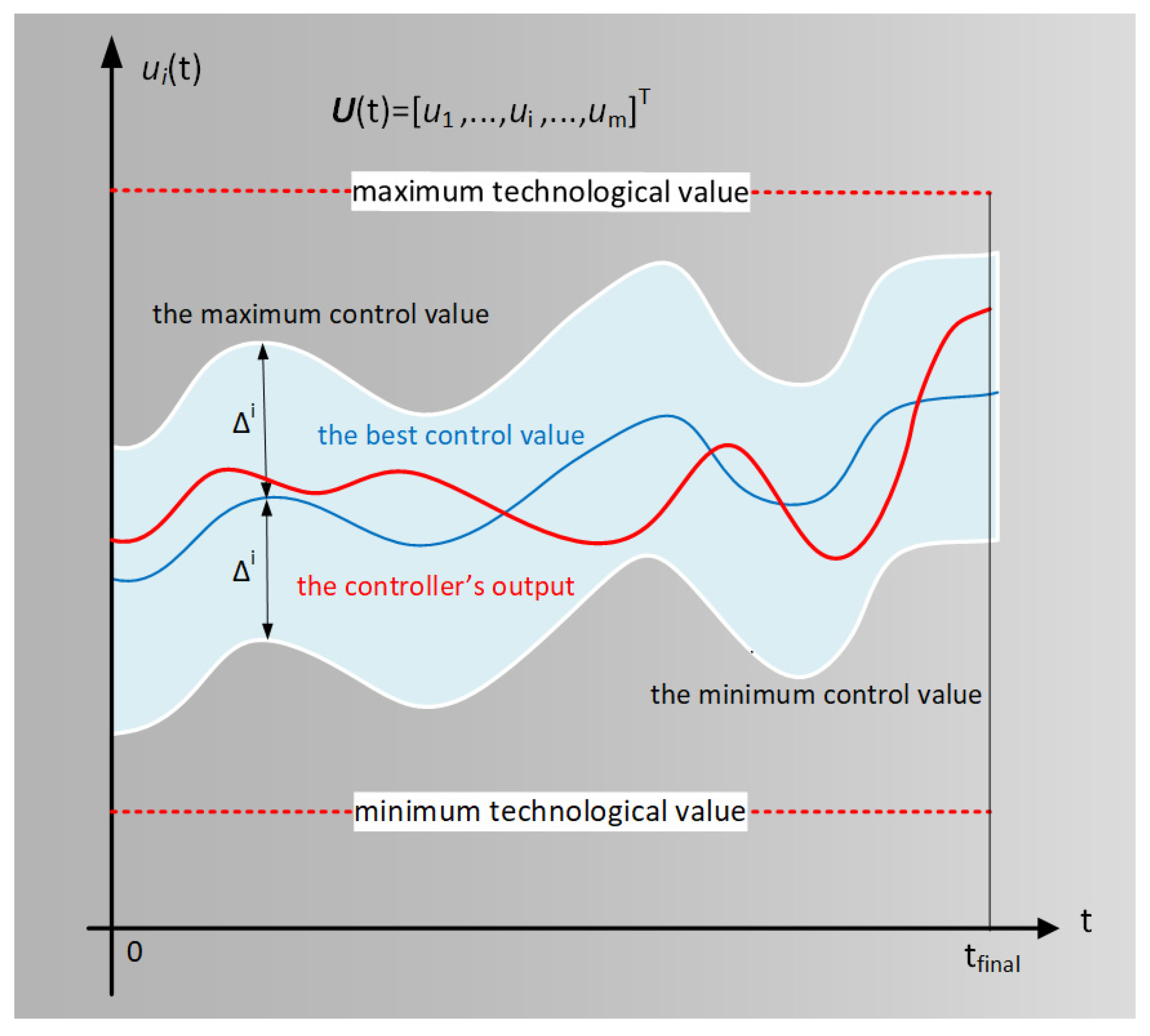
We recall the notion of a predefined control profile illustrated in Figure 1. This figure presents the evolution solely of the control output $u_i(t),1\le i\le m, t\in [0,t_{final}]$. The blue curve depicts a control profile as a continuous evolution of control output (against the controller). The control profile (CP) is supposed to be a “good” control output that determines even an optimal or a quasi-optimal performance index. Hence, it corresponds to an optimal or quasi-optimal solution to our control problem and will be called the reference CP in the sequel.

The red curve is the graphic representation of a real solution implemented through a closed-loop control structure. When the latter works well, this real solution is placed in a blue curve’s neighborhood, and a close performance index is expected. Figure 1 suggests a possible neighborhood, the blue zone, which is a “tube” around the optimal or quasi-optimal solution.

The main idea is to replace the interval ${\Omega }_i$ (see Equation (2)), which usually involves a too-large search space, with the domain represented by the blue zone. This neighborhood of the reference CP should be large enough to ensure metaheuristic algorithm convergence.

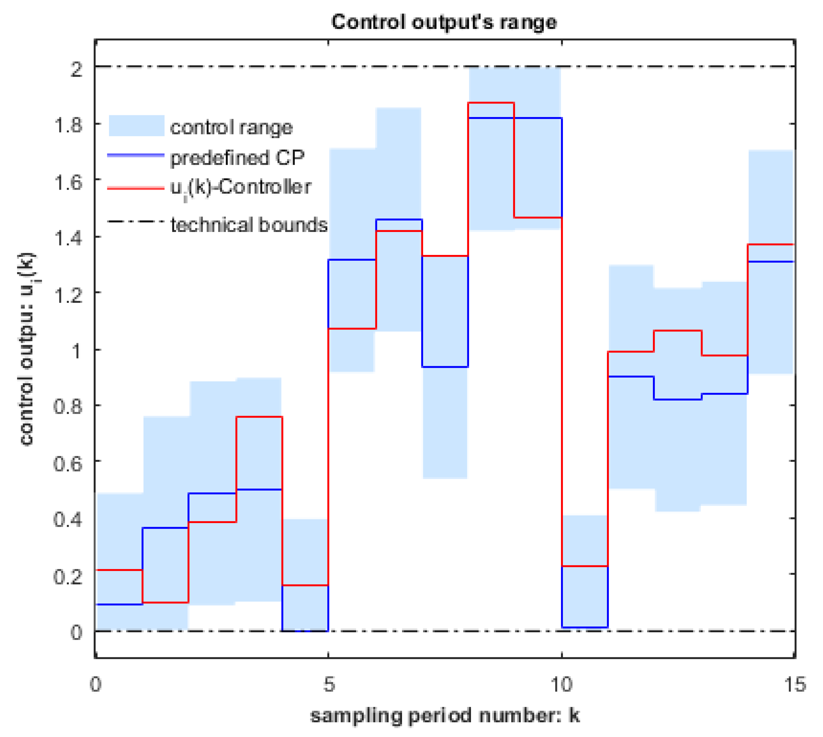
As mentioned in Section 2, we shall work with discrete values for time and control outputs. Figure 2 shows how the predefined CP principle can be illustrated in this situation.

Figure 2 uses an example from the paper [26] illustrating the positions of the predefined CP and control values inside the control ranges. For each sampling period, the intersection between the domain Ω_i and the blue zone from Figure 1 forms a blue rectangle referred to as the control range.

For example, the values ${\Delta }^i$ used to determine the control ranges may be calculated using Equation (5).

$${\Delta }^i=\alpha \left(u_{\max }^i-u_{\min }^i\right);\alpha =20\%$$

(5)

In Figure 2, considering α = 20% and the technical bounds 0 and 2, we have Δ = 0.4. Thus, the height of the blue rectangles would be 0.8. However, these control ranges cannot surpass technological limits. For this reason, some blue rectangles have their heights cut off at the upper or lower sides.

Remark 1:

The control range must be adapted for each sampling period $k, k=0,\cdots ,H-1$ and control input $u_i(t),1\le i\le m$ to implement the predefined CP.

The control range for the control output $i$ and moment $k$ is denoted $R^i\left(k\right)$ and determined by its height because its width is always the sampling period.

Remark 2:

In the sequel, a control range will be assimilated with the interval representing its height and denoted $R^i\left(k\right)$ as well.

Hence the control range for the moment k will generally be:

R_k = R¹(k) R²(k) … R^m(k).

(6)

Details concerning how the control range $R^i(k)$ is calculated in our case study will be given in Section 5.1.

Remark 3:

The smaller the value ${\Delta }^i$, the smaller extent of the new control range. However, a too-small ${\Delta }^i$ will cause the convergence to be lost. A realistic approach is to set ${\Delta }^i$ after a few simulations.

4. Predictions Based on Adaptive Particle Swarm Optimization Algorithm

This section presents the specific controller structure proposed in our work, having a few modules connected among them. A practical example is also given to demonstrate the systemic connections and prepare a case study for the execution time analysis.

4.1. Process Model, Constraints, and Performance Index

This section presents the process model, constraints, and performance index concepts using a specific OCP, which concerns a specific artificially lighted photobioreactor. As we have already mentioned, we are not interested in presenting this process to disclose its technological aspects but in describing a nontrivial process model and preparing a case study, in which we apply our execution time-decreasing method.

4.1.1. Process Model

This subsection presents the model of a continuously stirred flat-plate photobioreactor (PBR) lighted on one side for algae growth, whose physical and constructive parameters are presented in [23,31].

Because of the attenuation of the light inside the PBR, the latter’s dynamic model is a distributed-parameter system. The PBR’s depth, L, is discretized in $k_L$ points equally spaced ($z_i\in [0, L]$ $z_i, i=1,\dots ,k_L$) to convert this system into a lumped-parameter system. The resulting process model (PM) is presented hereafter:

$${\dot{x}}_1(t)=\left[{\mu }_{\max }\cdot \frac{1}{k_L}\cdot {\displaystyle \sum _{i=1}^{k_L}\frac{G_i(t)}{k_S+G_i(t)+\frac{1}{k_I}\cdot G_i{(t)}^2}}-{\mu }_d\right]\cdot x_1(t)$$

(7)

$${\dot{x}}_2(t)=A\cdot C\cdot q(t)$$

(8)

$$G_i(t)=q(t)\cdot k_i{}^{x_1(t)}, i=1,\dots ,k_L$$

(9)

$$k_i=e^{-\frac{1+\alpha }{2\alpha }\cdot E_a\cdot z_i}; i=1,\dots ,k_L$$

(10)

$$m(t)=V\cdot x_1(t)$$

(11)

The state variables have the following meaning:

$x_1(t)$: the biomass concentration (in g·/L);

$x_2(t)$: the amount of light that has illuminated the PBR up to moment t (in µmol/m²/s);

Equations (9) and (10) complete Equation (7) and are used, in different modules of our simulation programs, for the numerical integration.

The input variable q(t) is the incident light intensity and will be considered the control input and denoted by a consecrated notation:

u(t) = q(t)

(12)

Equation (11) calculates the biomass in the PBR, m(t), which can be considered an output variable because it is the PBR’s product.

Table A1. The constants of the PBR model.

radiative model	$E_a$ = 172 m2·kg−1	absorption coefficient
	$E_s$ = 870 m2·kg−1	scattering coefficient
	$b$ = 0.0008	backward scattering fraction
kinetic model	${\mu }_{max }$= 0.16 h−1	specific growth rate
	${\mu }_d$ = 0.013 h−1	specific decay rate
	$K_S$ = 120 µmol·m−2·s−1	saturation constant
	$K_I$ = 2500 µmol·m−2·s−1	inhibition constant
physical parameters	$V$ = 1.45·10−3 m3	the volume of the PBR
	L = 0.04 m	depth of the PBR
	A = 3.75·10−2 m2	lighted surface
	$x_0$ = 0.36 g/L	the initial biomass concentration
other constants	C = 3600·10−2	light intensity conversion constant
	$k_L$ = 100	number of discretization points
	$q_m=50{ \mathsf{\mu }\mathrm{mol}/\mathrm{m}}^2/\mathrm{s}$	lower technological light intensity
	$q_M=2000{ \mathsf{\mu }\mathrm{mol}/\mathrm{m}}^2/\mathrm{s}$	upper technological light intensity
	$m_0$ = 3 g.	the minimal final biomass

from Appendix A shows the constants used by the PM (7)–(11), avoiding their definitions, which are irrelevant to this work.

4.1.2. Constraints

Other elements that define an optimal control problem are the constraints. We denote by t₀ and t_f the initial and final moments of the control horizon.

In our case study, the following constraints must be met:

control horizon: t₀ ≤ t ≤ t_f, where t₀ = 0; t_f =120 h

(13)

$$\mathrm{initial} \mathrm{conditions}: x_1(t_0)=x_0; x_2(t_0)=0$$

(14)

bound constraints: q_m ≤ q(t) ≤ q_M, with t₀ ≤ t ≤ t_f.

(15)

As a productivity constraint, it is important to have minimal final biomass; that is,

$$m(t_f)\ge m_0,$$

(16)

where m₀ is the minimal newly produced biomass. Equivalently, it holds

$$x_1(t_f)\ge \frac{m_0}{V}.$$

(17)

Equation (9) can be seen as a path (state trajectory) constraint defining the admissible trajectories.

4.1.3. Performance Index

The third element defining an OCP is the performance index. This one supposes having a cost function associated with each admissible trajectory and the optimization sense (to find the minimum or maximum).

In our work, the cost function (18) minimizes the amount of light irradiating the PBR while constraint (10) is met. The setting of two weight factors ($w_1$ and $w_2$) is an important issue.

$$J(q(\cdot ), x_0)=w_1\cdot {\displaystyle {\int }_{t_0}^{t_f}q(t)\cdot dt}+w_2\left(m(t_f)-m_0\right).$$

(18)

In this context, the performance index has the following expression:

$$J^{*}(x_0)=\underset{q(t), t_0\le t\le t_f}{\min }J(q(\cdot ), x_0).$$

(19)

Solving the PBR optimal control problem means finding the optimal control sequence, which minimizes the cost function (18):

$$q^{*}(t), t_0\le t\le t_f.$$

(20)

Equations (18)–(20) are adapted below to our discretized RHC structure. When the prediction horizon is [k, H], the objective function that must be minimized (over the set of all predicted control sequences pcs(k)) is given by Equation (21).

$$J(k,x(k))=\underset{pcs(k)|{}_{m\left(H\right)\ge m_0}}{\min }\left\{w_1\cdot A\cdot C{\displaystyle \sum _{i=k}^{H-1}q(i)}+w_2\cdot \left[V\cdot x_1(H)-m_0\right]\right\}$$

(21)

Consequently, the optimal prediction is the following optimal control sequence:

$$\mathrm{ocs}(k)=\arg J(k,x(k)).$$

(22)

Hence, the current control output is the first element of the sequence $\mathrm{ocs}(k)$.

NB: We note that generating a closed-loop solution to this problem is more complex than finding the optimal control sequence (22).

4.2. Prediction-Based Controller Structure

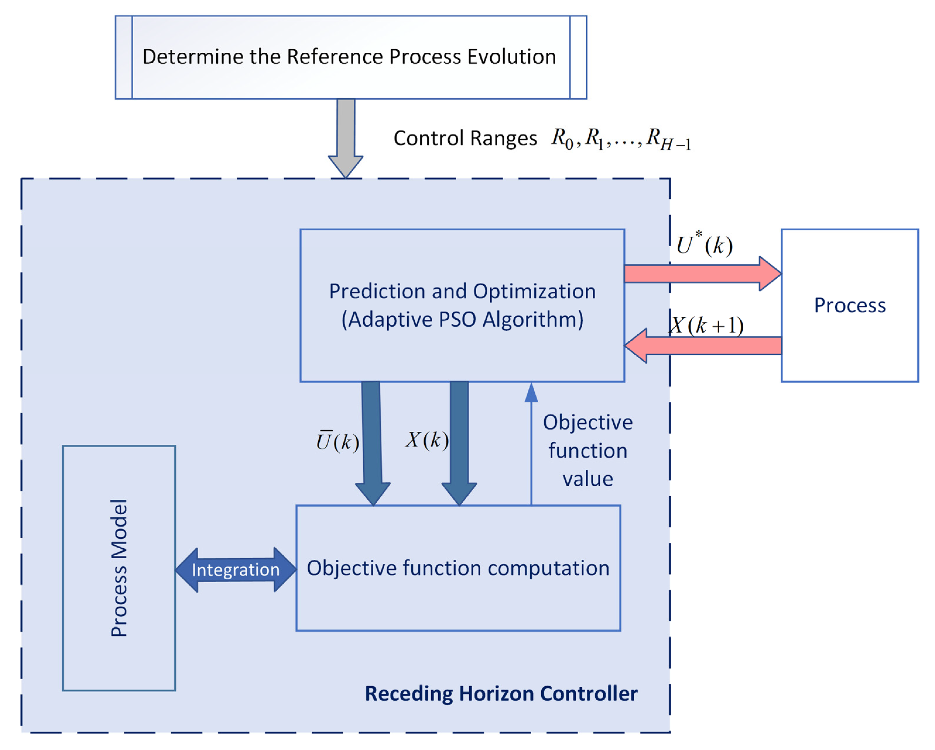
Section 3, together with the option of using the APSOA, leads to the general structure of the proposed controller presented in Figure 3.

Before including the APSOA in the controller, this algorithm is tested to discover whether it is suitable to solve the considered problem. Consequently, we obtain the best-known evolution of the process, which gives the best performance index. This optimal or quasi-optimal solution can be called “reference process evolution”. The best CP yielding the reference process evolution is recorded and used subsequently to generate the control ranges $R_0,R_1,\cdots ,R_{H-1}$. This CP is referred to as reference CP and denoted “Uref”.

The APSOA is integrated into the prediction module, called the predictor, in the sequel. At the moment $k,0\le k<H$, the predictor searches for the best prediction from the current state according to the control ranges $R_k,\cdots ,R_{H-1}$. Thus, the search space is less extended, being a neighborhood of the reference CP.

To do that, the predictor sends the current state vector $X(k)$ and a candidate prediction $\overline{U}(k)$ toward the “objective function computation” module. In turn, the latter frequently calls the PM for numerical integration.

The result is ocs(k), a control sequence with H-k control values for the remaining sampling periods. Its first element, $U^{*}(k)$, is the optimal control value that is sent toward the process. Data exchanged between the controller and the process are indicated by red arrows, which also close the control loop.

The well-known ASPOA (Adaptive Particle Swarm Optimization Algorithm) is presented in many papers [4,28,32]; paper [23] gives a comprehensive description of this algorithm in a similar context. The next section describes APSOA as a module of the controller proposed here.

5. Execution Time Decrease

This section is devoted to the predefined CP implementation and range tuning considering the OCP formulated in Section 3. Although our presentation considers some details of the solved problem, it can be applied to any other OCP with minor changes.

5.1. Implementation of the Predefined Control Profile

To prove the efficiency of our approach, we developed programs used in the sequel to conduct some simulation series, which are the topic of Section 6. Their algorithms are described below in a way that focuses on implementing control range adaptation and tuning.

Implementing the proposed method affects all three levels of our application schematically represented below (in order of calling):

$$\mathrm{CONTROLLER}\to \mathrm{PREDICTOR}\to \mathrm{APSOA}.$$

As we saw in Section 3, the employment of a predefined CP involves finally defining and using the control ranges. The proposed algorithms consider three modes of using the predefined CP:

mode = 1:	The control ranges are not used
mode = 2:	The closed-loop control adapts the control ranges
mode = 3:	The closed-loop control adapts and tunes the control ranges

The control range tuning will be described in Section 5.2.

Mode 1 corresponds to the situation described in our previous work [23], where the controller does not use a predefined CP.

Considering Remark 2 and the fact that m = 1, we can specify the limits of the interval representing a control range:

R_k = R¹(k) = [xm(k) xM(k)], k = 0,…,H − 1.

(23)

Thus, the vectors xm and xM store the lower and upper limits of the control ranges.

In mode = 2 and mode = 3, we consider these limits proportional to the predefined CP (called Uref) as below:

xm = (1 − p)·Uref;.

(24)

xM = (1 + p)·Uref.

(25)

The value p is constant, defining the neighborhood of Uref wherein control outputs take values. This value must be initialized; for example, p = 20%. Obviously, the values of vectors xm and xM must be truncated so as not to surpass the technological limits, denoted “qmin” and “qmax” (considering they are light intensities).

In mode = 1, because no control profile is used, the vectors xm and xM have all values equal to qmin and qmax, respectively.

With these specifications,

Table 1. Pseudo code of the CONTROLLER.

	Function CONTROLLER(k, mode)
	/* for simulation: CONTROLLER(k,X0,mode) */
	/* k—the current discrete moment */
1	#Initializations;        /*concerning the global constants*/
2	# Obtain the current state vector X(k)  /*In simulation, X0 is used instead */
3	If (mode = 1)         /*CR and tuning*/
4	xm(i) = qmin; i = 1,…,H.  /* qmin is the lower technological limit */
5	xM(i) = qmax; i = 1,…,H.  /* qmax is the upper technological limit */
6	else            /* mode = 2 or 3 */
7	xm = (1−p)·Uref;
8	xM = (1 + p)·Uref
9	# Truncate xm and XM not to overpass the technological limits.
10	end
11	ocs(k)$\leftarrow$PREDICTOR(k,X(k),mode)
12	U*(k)$\leftarrow$the first element of ocs(k)
13	# Send U*(k) toward the process /*the current optimal control value */
14	return             /* or wait for the next sampling period */

gives the controller algorithm related to the control structure from Figure 3.

Instruction #1 refers to initializing certain global constants and variables, especially concerning the predefined CP and PM. Instructions #3–#10 detail how the control ranges’ limits are set according to the chosen mode.

All preparatives lead to instruction #11, which is the call of the PREDICTOR function that returns the best prediction ocs(k). The latter’s first element is the optimal control value that will be sent to the process in the current sampling period.

The CONTROLLER is organized here as a function, but in our tests, it is included in the main simulation program.

Table 2. Algorithm of the function PREDICTOR.

	Function PREDICTOR(k, x0, mode)
	/* mode = 1: without control ranges; mode = 2: with control ranges; mode = 3: with control ranges and tuning; k—the current discrete moment; x0—the current state (biomass concentration)*/
1	Initializations;        /*space reservation for each particle*/
2	h$\leftarrow$H-k           /*h is the prediction horizon*/
3	xmh$\leftarrow$xm(k + 1,…,H);     /*copy h elements into the vector xmh */
4	xMh$\leftarrow$xM(k + 1,…,H);     /*copy h elements into the vector xMh */
5	Pgbest$\leftarrow$APSOA(k, h, x0, xmh, xMh, mode) /*call the metaheuristic */
6	ocs$\leftarrow$Pgbest
7	return ocs

shows the PREDICTOR’s algorithm conceived to prepare the function “APSOA” call. Each time is called, the APSOA function solves another optimization problem with another prediction horizon, “h”, and another current state,”x0”. The “mode” value is only transmitted to the APSOA function.

Instructions #3 and #4 construct the vectors xmh and xMh, which are the reduced version of xm and xM according to the h value. The function returns the global best prediction to the CONTROLLER.

As mentioned, the authors gave in [23] a comprehensive description of the APSOA, especially the movement particles’ equations and adaptive behavior implementation. Table 3 presents the new APSOA, which has two main characteristics:

• It keeps all the parts described in [23] concerning the adaptive behavior and movement equations. These parts are generically recalled (using the character #) to simplify the presentation, but they can be easily accessed.
• The algorithm’s new parts focus on the implementation of execution time decrease. Hence, the pseudo-code details the actions implementing the three modes of using control ranges.

APSOA is organized in the manner of a function of six input parameters, whose meaning results from the details already given. It calls the function “EvalFitnessJ”, which evaluates the objective function resulting from Equations (21) and (22).

Instructions #35–#41 constitute a group (shaded in dark grey) which is always executed when particles change position, whatever the mode. If the particles’ positions surpass the control range limits, the positions are truncated, and the velocity is reflected.

The algorithm’s main loop (instructions #13–#47), which implements the particles’ movement, uses the constant “stepM” representing the accepted maximum number of steps until convergence.

Table 3. Algorithm of the function APSOA (Adaptive Particle Swarm Optimization Algorithm).

	Function APSOA (k, h, x0, xmh, xMh, mode)
	Input parameters: k—the current discrete moment; x0—the current state (biomass concentration); h—predicted sequence length (particle’s positions Xi has h elements) xmh: vector with h elements—minimum value for each control range xMh: vector with h elements—maximum value for each control range
1	#General initializations;         /*space reservation for each particle*/
2	If (mode=3)               /*CR and tuning*/
3	#initialization step0 and $\Delta \mathrm{step}$
4	#initialization a /* e.g., 1/3, 1/4, 1/5,…*/
5	$\Delta \mathrm{m}\left(\mathrm{i}\right)\leftarrow \mathrm{a}\cdot \left(\mathrm{xmh}\right(\mathrm{i})-\mathrm{qmin}); \mathrm{i}=1,\cdots ,\mathrm{h}$ /* decrement step*/
6	$\Delta \mathrm{M}\left(\mathrm{i}\right)\leftarrow \mathrm{a}\cdot (\mathrm{qmax}-\mathrm{xMh}(\mathrm{i}\left)\right); \mathrm{i}=1,\cdots ,\mathrm{h}$ /* increment step*/
7	end
8	# Set the particles’ initial velocities, v(i,d), and positions $\mathrm{x}(\mathrm{i},\mathrm{d}), \mathrm{i}=1,\dots ,\mathrm{N}; \mathrm{d}=1,\dots ,\mathrm{h}$.
9	# For each particle, compute the best performance using the EvalFitnessJ function.
10	# Determine the position, Pgbest, and the value, GBEST, of the global best particle.
11	found$\leftarrow$0;       /* found =1 indicates the convergence of the algorithm*/
12	step$\leftarrow$1;
13	while (step < = stepM) & (found = 0)
14	/* stepM is the accepted maximum number of steps until convergence.*/
15	# Modify the coefficients that adapt the particles’ speed.
16	if (mode = 3) and (step > = step0) /*tuning of the Control Ranges */
17	for i = 1:h
18	xmh(i) = xmh(i)-$\Delta \mathrm{m}\left(\mathrm{i}\right)$
19	If (xmh(i) < qmin)
20	xmh(i) = qmin
21	end
22	xMh(i) = xMh(i) + $\Delta \mathrm{M}\left(\mathrm{i}\right)$
23	if (xMh(i) > qmax)
24	xMh(i) = qmax
25	end
26	end
27	step0$\leftarrow$step0 + $\Delta$step
28	end
29	for i = 1,…,N
30	#Compute the best local performance of particle i.
31	for d = 1,…,n
32	#Update the particle’s speed
33	#Speed limitation
34	#Update the particle’s position
35	if x(i,d) > xMh(d)
36	x(i,d)$\leftarrow$xMh(d)
37	v(i,d)$\leftarrow$-v(i,d)
38	elseif x(i,d) < xmh(d)
39	x(i,d)$\leftarrow$xmh(d)
40	v(i,d)$\leftarrow$-v(i,d)
41	end
42	end /*for d*/
43	#Compute fitness(i) and update the best performance of particle #i
44	#Update Pgbest, GBEST, and found
45	end /*for i*/
46	step$\leftarrow$step + 1;
47	end /*while*/
48	return Pgbest
49	end

Table 3. Algorithm of the function APSOA (Adaptive Particle Swarm Optimization Algorithm).

	Function APSOA (k, h, x0, xmh, xMh, mode)
	Input parameters: k—the current discrete moment; x0—the current state (biomass concentration); h—predicted sequence length (particle’s positions Xi has h elements) xmh: vector with h elements—minimum value for each control range xMh: vector with h elements—maximum value for each control range
1	#General initializations;         /*space reservation for each particle*/
2	If (mode=3)               /*CR and tuning*/
3	#initialization step0 and $\Delta \mathrm{step}$
4	#initialization a /* e.g., 1/3, 1/4, 1/5,…*/
5	$\Delta \mathrm{m}\left(\mathrm{i}\right)\leftarrow \mathrm{a}\cdot \left(\mathrm{xmh}\right(\mathrm{i})-\mathrm{qmin}); \mathrm{i}=1,\cdots ,\mathrm{h}$ /* decrement step*/
6	$\Delta \mathrm{M}\left(\mathrm{i}\right)\leftarrow \mathrm{a}\cdot (\mathrm{qmax}-\mathrm{xMh}(\mathrm{i}\left)\right); \mathrm{i}=1,\cdots ,\mathrm{h}$ /* increment step*/
7	end
8	# Set the particles’ initial velocities, v(i,d), and positions $\mathrm{x}(\mathrm{i},\mathrm{d}), \mathrm{i}=1,\dots ,\mathrm{N}; \mathrm{d}=1,\dots ,\mathrm{h}$.
9	# For each particle, compute the best performance using the EvalFitnessJ function.
10	# Determine the position, Pgbest, and the value, GBEST, of the global best particle.
11	found$\leftarrow$0;       /* found =1 indicates the convergence of the algorithm*/
12	step$\leftarrow$1;
13	while (step < = stepM) & (found = 0)
14	/* stepM is the accepted maximum number of steps until convergence.*/
15	# Modify the coefficients that adapt the particles’ speed.
16	if (mode = 3) and (step > = step0) /*tuning of the Control Ranges */
17	for i = 1:h
18	xmh(i) = xmh(i)-$\Delta \mathrm{m}\left(\mathrm{i}\right)$
19	If (xmh(i) < qmin)
20	xmh(i) = qmin
21	end
22	xMh(i) = xMh(i) + $\Delta \mathrm{M}\left(\mathrm{i}\right)$
23	if (xMh(i) > qmax)
24	xMh(i) = qmax
25	end
26	end
27	step0$\leftarrow$step0 + $\Delta$step
28	end
29	for i = 1,…,N
30	#Compute the best local performance of particle i.
31	for d = 1,…,n
32	#Update the particle’s speed
33	#Speed limitation
34	#Update the particle’s position
35	if x(i,d) > xMh(d)
36	x(i,d)$\leftarrow$xMh(d)
37	v(i,d)$\leftarrow$-v(i,d)
38	elseif x(i,d) < xmh(d)
39	x(i,d)$\leftarrow$xmh(d)
40	v(i,d)$\leftarrow$-v(i,d)
41	end
42	end /*for d*/
43	#Compute fitness(i) and update the best performance of particle #i
44	#Update Pgbest, GBEST, and found
45	end /*for i*/
46	step$\leftarrow$step + 1;
47	end /*while*/
48	return Pgbest
49	end

5.2. Tuning of Control Ranges

Before calling the predictor, the controller adapts the established control ranges to each sampling period (instructions #3–#10). Lower and upper limits are assigned to each control output and each prediction horizon step. Thus, the intervals’ limits have initial values.

A compelling situation is when the current state is very different from the PM state due to important perturbations of any sort. The APSOA may not converge using the initial limits, but rather stops at a best-found solution. The PREDICTOR will return the control sequence ocs(k) that would not generate a state trajectory “neighboring” the reference trajectory (i.e., the trajectory of the PM yielded by the reference CP).

The solution is to adjust the intervals’ limits after a certain number of steps until the convergence should have been ascertained. In other words, the predictor will tune the control ranges modifying the initial intervals’ limits. Moreover, the tunning action may gradually increase the control ranges’ sizes so as not to lose the convergence of the APSOA.

The instructions of APSOA to achieve the control range tuning are shaded in light grey. Some initializations are performed by instructions #2–#7. The tuning of intervals uses decrement and increment steps defined below, respectively:

$$\Delta \mathrm{m}\left(\mathrm{i}\right)\leftarrow \mathrm{a}\cdot \left(\mathrm{xmh}\right(\mathrm{i})-\mathrm{qmin}); \mathrm{i}=1,\cdots ,\mathrm{h}$$

(26)

$$\Delta \mathrm{M}\left(\mathrm{i}\right)\leftarrow \mathrm{a}\cdot (\mathrm{qmax}-\mathrm{xMh}(\mathrm{i}\left)\right); \mathrm{i}=1,\cdots ,\mathrm{h}$$

(27)

The constant “a” has values such as 1/3, 1/4, 1/5 and so on. In this way, the difference between the control range lower (upper) limit and the technological lower (upper) limit can be progressively covered by a few adjustments. The decrement and increment steps are computed only once using the initial values of xmh(i) and xMh(i).

The adjustment of the control range (instruction #16–#28) is performed when the step number, “step”, equals a predefined number, “step0”, using the following equations:

$$\mathrm{xmh}\left(\mathrm{i}\right)=\mathrm{xmh}\left(\mathrm{i}\right)-\Delta \mathrm{m}\left(\mathrm{i}\right)$$

(28)

$$\mathrm{xMh}\left(\mathrm{i}\right)=\mathrm{xMh}\left(\mathrm{i}\right)+\Delta \mathrm{M}\left(\mathrm{i}\right)$$

(29)

The values of “step0” and “$\Delta$step” are initialized in instruction #3 following some simulations. The reader will find proper values for our OCP in the programs attached as Supplementary Materials.

Remark 4:

The APSOA performs the tuning action gradually to allow the search process to extend as less as possible. In this way, there will be a benefit in terms of execution time.

6. Simulation Results and Discussion

This section presents a simulation study concerning the closed-loop optimal control of the process described in the OCP stated in Section 4.1. The algorithms CONTROLLER, PREDICTOR, and APSOA, developed in the previous section, have been used to implement and simulate the control structure. The simulations must allow the execution time evaluation to validate the proposed decreasing method. Concretely, our simulation study has the following goals:

• To implement the closed-loop structure using the algorithms mentioned above.
• To implement the three algorithms, CONTROLLER, PREDICTOR, and APSOA, to cope with the three modes of using the control profile.
• To confirm that the proposed technique works properly and decreases the execution time.

The authors have addressed the first objective in [23], but in another context. In addition, the control ranges’ adaptation and tuning have important repercussions on the structure and implementation of the algorithms and programs.

A general program emulates the working of the entire closed-loop control structure. It is written using MATLAB language and system and allows us to achieve the simulation study. The pseudo-code of this program is given in Appendix B.

All the modules depicted in Figure 3 have associated program units. The CONTROLLER integrates the PM, subjected to Equations (7)−(11), and sends the optimal control output toward the process. The latter also is emulated by a simulation module, which in this study is identical to the PM. This choice is not a simplification that guarantees the success of our simulations. We should not expect that the simulated process tracks the reference trajectory, implicitly expressed by the reference CP, because of two factors:

• The closed loop does not work identically with the open loop. We recall that the reference CP can be assimilated to an open-loop solution of the OCP at hand.
• The APSOA is a stochastic algorithm that finds quasi-optimal solutions not identical to the reference CP.

Moreover, in this simulation study, we are not interested in evaluating the consequences of a process different from the PM but in evaluating the control range’s adaptation end tuning.

6.1. Execution Time Evaluation

The closed-loop structure makes a computational effort to optimally control the process in a sense defined by the OCP. We are interested in estimating this effort during the entire control horizon. The third objective of our simulation study means that the controller’s execution time must be evaluated for the three CONTROLLER utilization modes.

The APSOA has two parts, the initialization part (see Table 3, lines #1–#12) and the “while” loop (lines #13–#47). Its execution has a stochastic character, but for a specific realization of this stochastic process, we can give the “a posteriori” execution time “ExT”:

$$ExT=n_1+N\cdot D+Nsteps\cdot (n_2+N\cdot D)$$

(30)

The values n₁ and n₂ represent the durations of the elementary actions (assignments, tests, etc., except the objective function calls) included in the previously mentioned parts, expressed in time units. D is the duration of the objective function (EvalFitnessJ) execution, which in this context is practically constant. Nsteps denotes the step number until stop-criterion fulfilment. Using the APSOA in our computation context has a particularity: the process integration needs much greater execution time than the other parts of the algorithm. Because we have $n_1,n_2<<N\cdot D$, it holds:

$$ExT\approx (Nsteps+1)\cdot N\cdot D=Ncalls\cdot D$$

(31)

considering that “Ncalls” is the number of calls of the objective function during the APSOA’s running.

Equation (31) justifies why, in previous works, we have used an empirical measure of execution time, which means counting the objective (cost) function calls throughout the control horizon. In our case, the simulation program counts the number of calls of the “EvalFitnessJ” function during the control horizon [0 H]. The number of calls is cumulated for all sampling periods and divided by H at the end; the average number of calls is more appropriate for comparisons and is also denoted “Ncalls” from here on.

The value of Ncalls is an empirical measure of the implemented algorithms’ execution time. Of course, it depends on the number of steps until convergence, which, in turn, can be influenced by the integration method and its parameters. Nevertheless, when it is obtained in similar conditions, Ncalls helps us to compare the proposed algorithms from the point of view of execution time: its decrease means the execution time decrease.

The CONTROLLER and PREDICTOR inherit the stochastic character from the APSOA. For this reason, the simulation program was carried out 30 times such that a statistical analysis could be done. Details concerning the simulation program are given in Appendix C.

6.2. Simulation without Range Adaptation

The first implementation of the simulation program calls the CONTROLLER with mode = 1; that is, it does not adapt the control ranges and considers the technological bound uniquely. Thus, the first simulation series consisted of 30 runs of this program and yielded the data reported in

Table 4. Simulation series for closed loop without control ranges.

Run #	J	Ncalls	Run #	J	Ncalls
1	9.0136	960	16	9.2717	672
2	9.0423	665	17	9.3212	727
3	9.0523	951	18	9.2314	689
4	9.0448	845	19	9.2276	758
5	9.1961	940	20	9.2726	731
6	8.9792	962	21	9.2753	848
7	9.1024	663	22	9.3992	717
8	9.0728	959	23	9.2007	738
9	9.0605	841	24	9.2302	839
10	9.0059	941	25	9.4145	654
11	9.3527	773	26	9.4045	745
12	9.4327	662	27	9.2029	759
13	9.2569	747	28	9.4126	753
14	9.2506	785	29	9.2264	798
15	9.4629	812	30	9.2924	790

(following the procedure given in Appendix C.1).

The results of the simulation series are presented in Table 4, where the average number of calls is shown in the “Ncalls” columns and calculated by dividing the cumulated call number by 120 (the sampling period number). The columns denoted J give us the performance index.

Table 5. Statistics on the performance index.

Jmin	Javg	Jmax	Sdev	Jtypical
8.979	9.224	9.463	0.142	9.226

shows some statistical values concerning the performance index: the minimum, average, maximum, standard deviation (Sdev), and typical values.

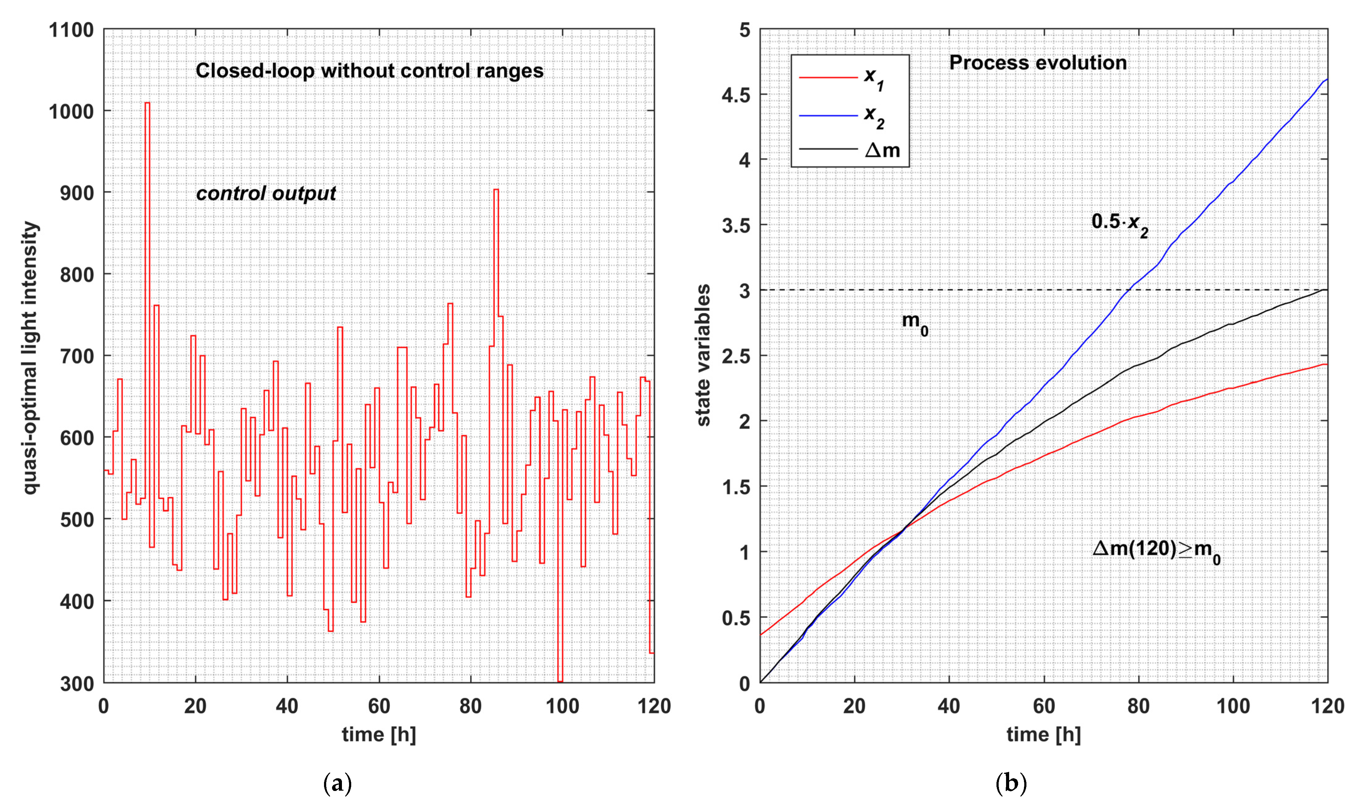
We consider a specific execution as “typical execution” when its performance index has the closest value to “Javg”. In our case, the typical execution is the 29th and is plotted in Figure 4. The CONTROLLER with mode = 1 generates the control values from Figure 4a. The typical state evolution of the process is given in Figure 4b.

Ncalls = 798 can be a “measure” of the typical execution time. This measure has the advantage of not depending on the hardware’s characteristics.

To reinforce our analysis based on Ncalls, we also measured the real execution times for thirty runs (different from Table 4). The processor we have used in our simulations is an Intel Core i7-6700HQ [email protected] GHz, and the PM was integrated using the functions of the MATLAB system.

Table 6. Execution times for the closed loop without control ranges.

Run #	ExTime	Run #	ExTime	Run #	ExTime
1	890.8	11	771.2	21	892.6
2	796.5	12	858.8	22	902.5
3	855.7	13	880.2	23	898.4
4	845.2	14	947.	24	878.8
5	924.3	15	894.4	25	938.7
6	861.	16	750.8	26	798.
7	910.5	17	1022.9	27	879.5
8	879.5	18	895.7	28	904.2
9	901.3	19	854.9	29	831.
10	854.8	20	1009.3	30	898.1

presents these execution times in columns called “ExTime”.

It holds:

average ExTime = 880.9 s.

(32)

We must verify that the proposed techniques shorten this duration.

6.3. Simulation of Closed-Loop Working with Control Ranges Adaptation

In the second simulation series, each execution called the CONTROLLER with mode = 2 and adapted the control ranges according to the reference CP. These simulations yielded the data reported in

Table 7. Simulation series for closed loop with control ranges.

Run #	J	Ncalls	Run #	J	Ncalls
1	9.1501	530	16	9.1549	666
2	9.1695	591	17	9.1715	566
3	9.1828	511	18	9.1572	619
4	9.1377	569	19	9.1775	505
5	9.1786	656	20	9.1112	644
6	9.1506	563	21	9.1682	654
7	9.2067	623	22	9.1841	507
8	9.155	624	23	9.1643	552
9	9.1398	591	24	9.169	540
10	9.1751	595	25	9.1868	611
11	9.1937	596	26	9.1607	576
12	9.1627	511	27	9.1544	520
13	9.2359	713	28	9.1786	633
14	9.1701	602	29	9.1897	601
15	9.1822	563	30	9.1788	635

(following the procedure given in Appendix C.2).

Table 8. Statistics on the performance index (mode = 2).

Jmin	Javg	Jmax	Sdev	Jtypical
9.111	9.170	9.236	0.023	9.170

presents similar statistics as Table 5 but uses data from Table 7.

This time, the typical execution is the 14th of Table 7. Thus, Ncalls = 602 can characterize the typical execution time in this case.

The standard deviation of J is 0.023, much less than 0.142 (for mode = 1). This fact has a logical explanation: the domain between technological bounds is more extended that the union of control ranges. As a repercussion, the values of the performance index are also less spread out.

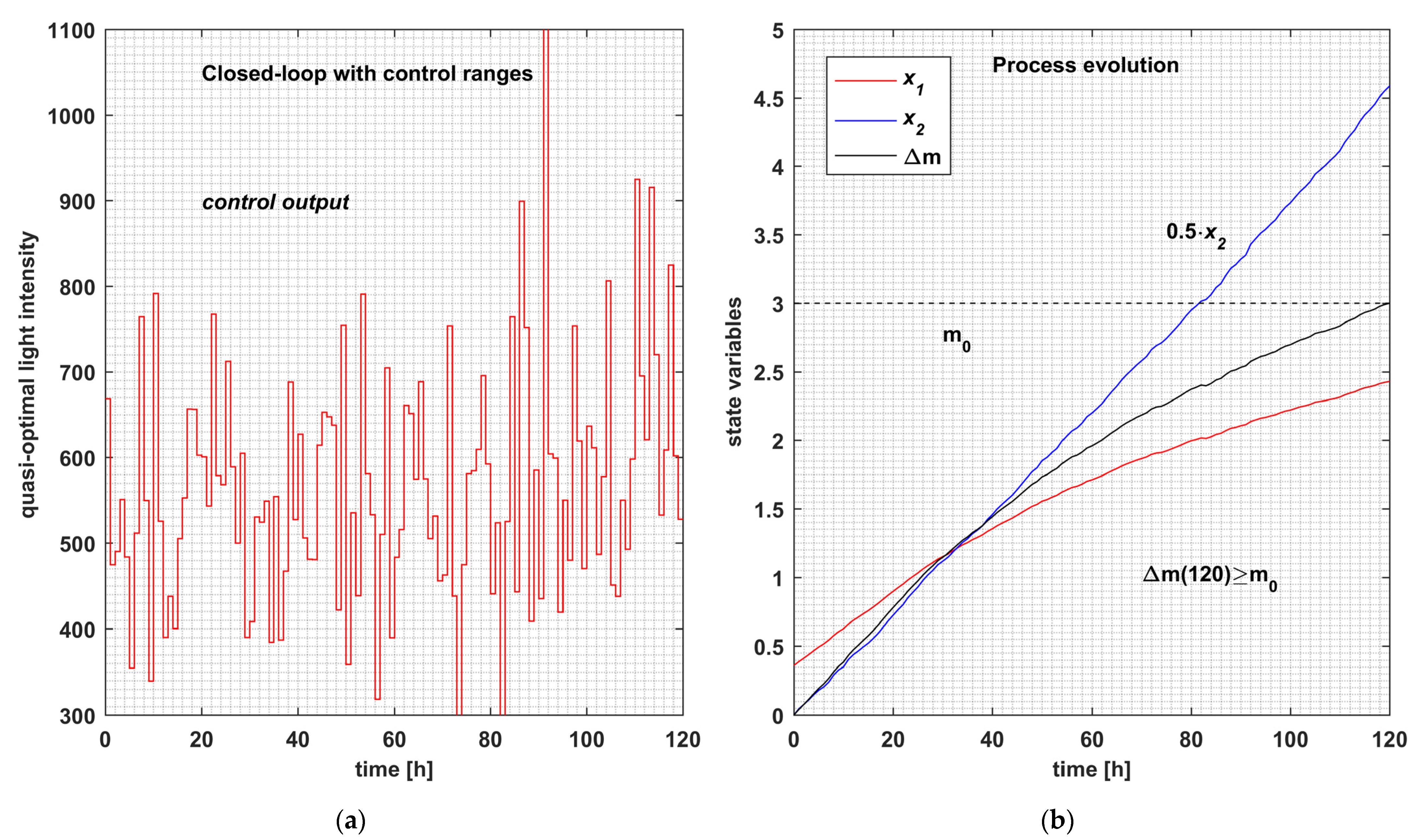
The typical execution is plotted in Figure 5. The CONTROLLER with mode = 2 generates the control values from Figure 5a. The process’ typical state evolution is given in Figure 5b.

Remark 5:

• Figure 4 and Figure 5 have the same aspect, meaning that the closed loops work similarly.
• The controller with mode = 2 works properly, as in mode = 1, but faster. All the constraints are fulfilled.
• The controller with control range adaptation decreased the execution time because Ncalls diminished by 24.5% compared to the controller with mode = 1.

For the simulation series presented in Table 7, we also measured the total execution time for the thirty runs, 22,131.5 s. This measure allowed us to calculate the

average ExTime = 737.7 s.

(33)

In the hardware context presented before, the average execution time decreased from 880.9 (see (32)) to 737.7, which means a diminution of 16.2% compared to the controller without control ranges. This percentage is less than that indicated in Remark 5, because Equation (31) approximates ExT. Nevertheless, this remark is in agreement with the real tendency.

6.4. Simulation of Closed-Loop Working with Control Range Adaptation and Tuning

In the third simulation series, each execution called the CONTROLLER (with mode = 3) to adapt and tune the control ranges. These simulations yielded the data reported in

Table 9. Simulation series for the closed loop with control ranges and tuning.

Run #	J	Ncalls	Run #	J	Ncalls
1	9.1879	672	16	9.1943	633
2	9.1742	538	17	9.1714	581
3	9.1759	717	18	9.1742	569
4	9.1834	639	19	9.1548	605
5	9.1504	652	20	9.1672	621
6	9.1713	630	21	9.1353	537
7	9.1615	523	22	9.1582	611
8	9.1423	508	23	9.1765	670
9	9.1712	577	24	9.2054	554
10	9.1739	608	25	9.1333	705
11	9.1916	613	26	9.1832	547
12	9.1639	571	27	9.2009	643
13	9.1728	774	28	9.1935	585
14	9.1775	501	29	9.1443	592
15	9.1736	673	30	9.1785	599

(using the procedure given in Appendix C.3).

The data included in this table were used to compute the statistics displayed in

Table 10. Statistics on the performance index (mode = 3).

Jmin	Javg	Jmax	Sdev	Jtypical
9.133	9.171	9.205	0.018	9.171

(as in Table 5).

This time, the typical execution is the 17th of Table 9. Thus, Ncalls = 581 can characterize the typical execution time when mode = 3.

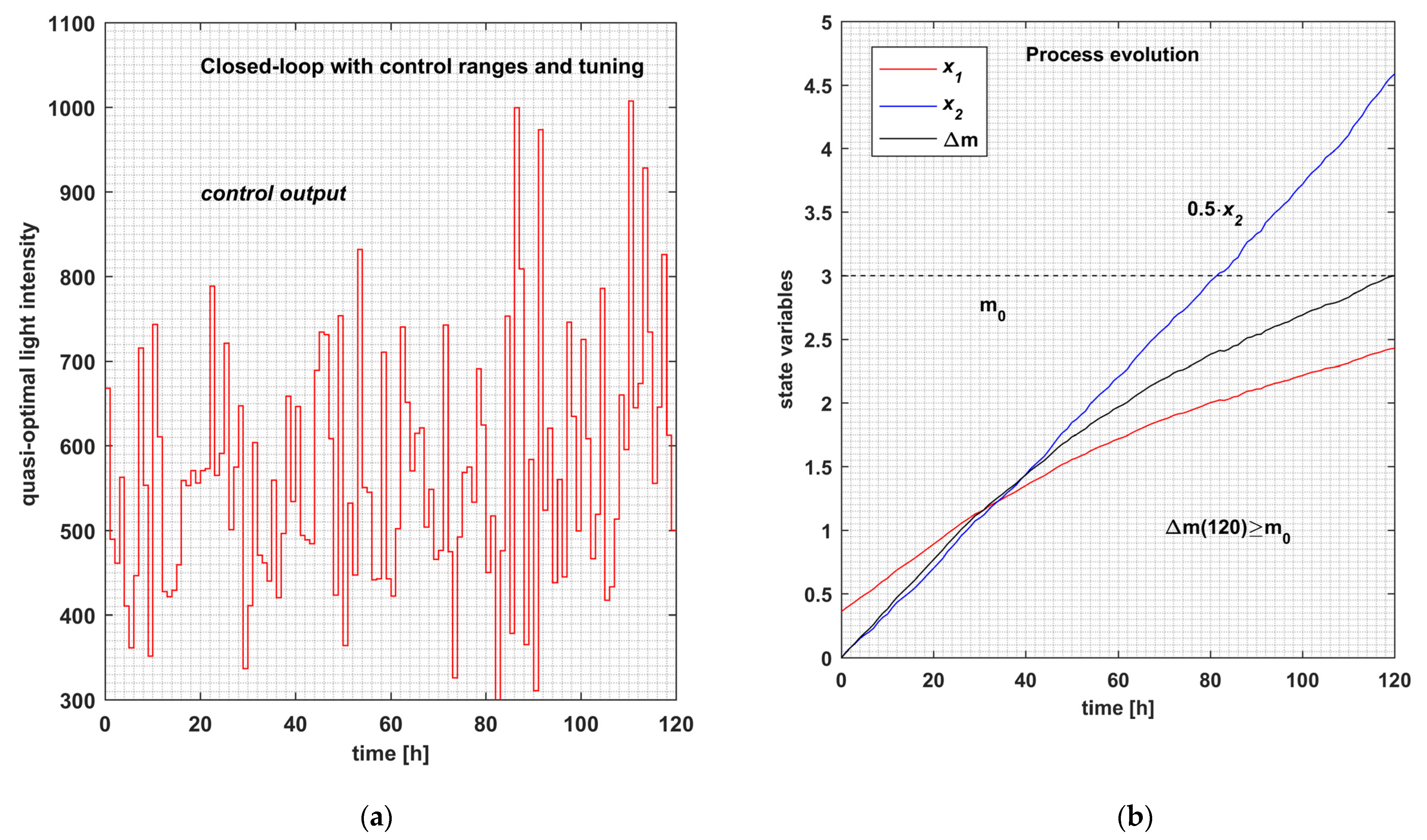
The typical execution is plotted in Figure 6. The CONTROLLER with mode = 3 generates the control values from Figure 6a. The process’ typical state evolution is given in Figure 6b.

The standard deviation of J is 0.018, practically equal to 0.023 (for mode = 2). The situations when the control ranges must be tuned are infrequent; that is, they occur when the current state is distant from the reference state trajectory. Only in those cases are the control ranges extended to conserve convergence. For this reason, the standard deviations are practically equal. On the other side, although rare, these situations decrease the execution time, because Ncalls diminishes from 602 to 581. It decreases by 3.5% compared to the controller with mode = 2, and by 27.1% against the first controller (mode = 1).

Remark 6:

• Figure 4 and Figure 6 have the same aspect, meaning that the closed loops work similarly.
• The controller with mode = 3 works properly, as in mode = 1, but faster. All the constraints are fulfilled.
• The controller with control range adaptation decreased the execution time, because Ncalls diminished by 27.1% compared to the controller with mode = 1.

As in previous subsections, we also measured the real execution times for thirty runs (different from Table 9).

Table 11. Execution times for the closed loop with control ranges and tuning.

Run #	ExTime [s]	Run #	ExTime [s]	Run #	ExTime [s]
1	696.01	11	656.02	21	606.25
2	778.46	12	681.86	22	601.70
3	736.75	13	828.09	23	812.89
4	665.94	14	745.42	24	754.47
5	843.31	15	823.66	25	616.89
6	851.08	16	779.48	26	591.39
7	712.82	17	670.01	27	699.41
8	724.09	18	742.59	28	786.92
9	665.91	19	750.33	29	641.37
10	642.30	20	713.98	30	745.00

presents the results.

This measure allowed us to calculate the

average ExTime = 718.8 s.

(34)

In the same hardware context presented before, the average execution time decreased from 880.9 (see (32)) to 718.8, which means a diminution of 18.4% compared to the controller with mode = 1. This percentage is less than that indicated in Remark 6 for the same reason mentioned before. Nevertheless, this remark is in agreement with the real tendency.

The real values of the average execution time for the three simulation series are summarized in

Table 12. Average execution time for the three simulation series.

Controller Type	Average Execution Time [s]
Controller without control range adaptation	878.7
Controller with control range adaptation	737.7
Controller with control range adaptation and tuning	718.8

.

The conclusion of our analysis based on Ncalls corresponds to the data from Table 12: the execution time decreased, as mentioned previously.

7. Conclusions

In the context of optimal control using a new technique based on reference CP, we presented implementation aspects that led to an execution time decrease when using metaheuristic algorithms.

Previous work has used predictions based on evolutionary algorithms integrated into an RHC structure, able to implement the control range adaptation. This paper adopted the same scientific context and treated two new general aspects:

• The APSOA was used as the metaheuristic generating the optimal predictions.
• A new technique, the tuning of control ranges, was proposed and integrated into the controller.

A simulation study was conducted to validate the contributions using a case study. The PM was a nontrivial dynamic system that stemmed from a distributed-parameter system. Looking at the simulation’s goals listed in Section 6, we can draw some conclusions:

• The APSOA was modified to include actions necessary to implement control ranges adaptation and tuning.
• Besides the new APSOA, the modules CONTROLLER and PREDICTOR were implemented to work according to three use modes: without control range adaptation, with control range adaptation, and with control range adaptation and tuning.
• A general simulation program was implemented, and three simulation series were carried out for each mode.

The controller converged for all simulations and sampling periods, and the closed loop worked properly with good performance index values. The control range adaptation and tuning determined the number of calls to decrease, so the controller’s execution time was reduced.

Although the tuning action rarely occurs, it causes the state trajectory to neighbor the reference trajectory, and consequently causes the performance index to preserve a quasi-optimal value.

The comparative analysis proved that the control range adaptation and tuning are effective, and the execution time decrease is significant. The interested reader can thoroughly understand and use the algorithms presented in this work, including the written programs attached as Supplementary Materials.

References

- Valadi, J.; Siarry, P. Applications of Metaheuristics in Process Engineering; Springer International Publishing: Berlin/Heidelberg, Germany, 2014; pp. 1–39. [Google Scholar] [CrossRef]
- Faber, R.; Jockenhövelb, T.; Tsatsaronis, G. Dynamic optimization with simulated annealing. Comput. Chem. Eng. 2005, 29, 273–290. [Google Scholar] [CrossRef]
- Onwubolu, G.; Babu, B.V. New Optimization Techniques in Engineering; Springer: Berlin/Heidelberg, Germany, 2004. [Google Scholar]
- Minzu, V.; Riahi, S.; Rusu, E. Optimal control of an ultraviolet water disinfection system. Appl. Sci. 2021, 11, 2638. [Google Scholar] [CrossRef]
- Banga, J.R.; Balsa-Canto, E.; Moles, C.G.; Alonso, A. Dynamic optimization of bioprocesses: Efficient and robust numerical strategies. J. Biotechnol. 2005, 117, 407–419. [Google Scholar] [CrossRef] [PubMed]
- Talbi, E.G. Metaheuristics—From Design to Implementation; Wiley: Hoboken, NJ, USA, 2009; ISBN 978-0-470-27858-1. [Google Scholar]
- Siarry, P. Metaheuristics; Springer: Berlin/Heidelberg, Germany, 2016; ISBN 978-3-319-45403-0. [Google Scholar]
- Kruse, R.; Borgelt, C.; Braune, C.; Mostaghim, S.; Steinbrecher, M. Computational Intelligence—A Methodological Introduction, 2nd ed.; Springer: Berlin/Heidelberg, Germany, 2016. [Google Scholar] [CrossRef]
- Mayne, D.Q.; Michalska, H. Receding Horizon Control of Nonlinear Systems. IEEE Trans. Autom. Control. 1990, 35, 814–824. [Google Scholar] [CrossRef]
- Goggos, V.; King, R. Evolutionary predictive control. Comput. Chem. Eng. 1996, 20 (Suppl. S2), S817–S822. [Google Scholar] [CrossRef]
- Hu, X.B.; Chen, W.H. Genetic algorithm based on receding horizon control for arrival sequencing and scheduling. Eng. Appl. Artif. Intell. 2005, 18, 633–642. [Google Scholar] [CrossRef] [Green Version]
- Hu, X.B.; Chen, W.H. Genetic algorithm based on receding horizon control for real-time implementations in dynamic environments. In Proceedings of the 16th Triennial World Congress, Prague, Czech Republic, 4–8 July 2005; Elsevier IFAC Publications: Amsterdam, The Netherlands, 2005. [Google Scholar]
- Minzu, V.; Serbencu, A. Systematic procedure for optimal controller implementation using metaheuristic algorithms. Intell. Autom. Soft Comput. 2020, 26, 663–677. [Google Scholar] [CrossRef]
- Chiang, P.-K.; Willems, P. Combine Evolutionary Optimization with Model Predictive Control in Real-time Flood Control of a River System. Water Resour. Manag. 2015, 29, 2527–2542. [Google Scholar] [CrossRef]
- Minzu, V. Quasi-optimal character of metaheuristic-based algorithms used in closed-loop—Evaluation through simulation series. In Proceedings of the ISEEE, Galati, Romania, 18–20 October 2019. [Google Scholar]
- Abraham, A.; Jain, L.; Goldberg, R. Evolutionary Multiobjective Optimization—Theoretical Advances and Applications; Springer: Berlin/Heidelberg, Germany, 2005; ISBN 1-85233-787-7. [Google Scholar]
- Minzu, V. Optimal Control Implementation with Terminal Penalty Using Metaheuristic Algorithms. Automation 2020, 1, 48–65. [Google Scholar] [CrossRef]
- Vlassis, N.; Littman, M.L.; Barber, D. On the computational complexity of stochastic controller optimization in POMDPs. ACM Trans. Comput. Theory 2011, 4, 1–8. [Google Scholar] [CrossRef] [Green Version]
- de Campos, C.P.; Stamoulis, G.; Weyland, D. The computational complexity of Stochastic Optimization. In Combinatorial Optimization; Fouilhoux, P., Gouveia, L., Mahjoub, A., Paschos, V., Eds.; ISCO. Lecture Notes in Computer Science; Springer: Cham, Switzerland, 2014; Volume 8596. [Google Scholar] [CrossRef] [Green Version]
- Sohail, M.S.; Saeed, M.O.; Rizvi, S.Z.; Shoaib, M.; Sheikh, A.U. Low-Complexity Particle Swarm Optimization for Time-Critical Applications. arXiv 2014. [Google Scholar] [CrossRef]
- Chopara, A.; Kaur, M. Analysis of Performance of Particle Swarm Optimization with Varied Inertia Weight Values for solving Travelling Salesman Problem. Int. J. Hybrid Inf. Technol. 2016, 9, 165–172. [Google Scholar] [CrossRef]
- Sethi, A.; Kataria, D. Analyzing Emergent Complexity in Particle Swarm Optimization using a Rolling Technique for Updating Hyperparameter Coefficients. Procedia Comput. Sci. 2021, 193, 513–523. [Google Scholar] [CrossRef]
- Minzu, V.; Ifrim, G.; Arama, I. Control of Microalgae Growth in Artificially Lighted Photobioreactors Using Metaheuristic-Based Predictions. Sensors 2021, 21, 8065. [Google Scholar] [CrossRef] [PubMed]
- Minzu, V.; Arama, I. Optimal Control Systems Using Evolutionary Algorithm-Control Input Range Estimation. Automation 2022, 3, 95–115. [Google Scholar] [CrossRef]
- Minzu, V.; Riahi, S.; Rusu, E. Implementation aspects regarding closed-loop control systems using evolutionary algorithms. Inventions 2021, 6, 53. [Google Scholar] [CrossRef]
- Minzu, V.; Georgescu, L.; Rusu, E. Predictions Based on Evolutionary Algorithms Using Predefined Control Profiles. Electronics 2022, 11, 1682. [Google Scholar] [CrossRef]
- Kennedy, J.; Eberhart, R.; Shi, Y. Swarm Intelligence; Morgan Kaufmann Academic Press: Cambridge, MA, USA, 2001. [Google Scholar]
- Beheshti, Z.; Shamsuddin, S.M.; Hasan, S. Memetic binary particle swarm optimization for discrete optimization problems. Inf. Sci. 2015, 299, 58–84. [Google Scholar] [CrossRef]
- Maurice, C. L’Optimisation par Essaims Particulaires-Versions Paramétriques et Adaptatives; Hermes Lavoisier: Paris, France, 2005. [Google Scholar]
- Minzu, V.; Barbu, M.; Nichita, C. A Binary Hybrid Topology Particle Swarm Optimization Algorithm for Sewer Network Discharge. In Proceedings of the 19th International Conference on System Theory, Control and Computing (ICSTCC), Cheile Gradistei, Romania, 14–16 October 2015; pp. 627–634, ISBN 9781479984800. [Google Scholar]
- Tebbani, S.; Titica, M.; Ifrim, G.; Caraman, S. Control of the Light-to-Microalgae Ratio in a Photobioreactor. In Proceedings of the 18th International Conference on System Theory, Control and Computing, ICSTCC, Sinaia, Romania, 17–19 October 2014; pp. 393–398. [Google Scholar]
- Beheshti, Z.; Shamsuddin, S.M. Non-parametric particle swarm optimization for global optimization. Appl. Soft Comput. 2015, 28, 345–359. [Google Scholar] [CrossRef]