Robust Control and Active Vibration Suppression in Dynamics of Smart Systems

Abstract

Challenging issues arise in the design of control strategies for piezoelectric smart structures. Piezoelectric materials have been investigated for use in distributed parameter systems in order to provide active control efficiently and affordably. In the active control of dynamic systems, distributed sensors and actuators can be created using piezoelectric materials. The three fundamental issues that structural control engineers must face when creating robust control laws are structural modeling methodologies, uncertainty modeling, and robustness validation. These issues are reviewed in this article. A smart structure with piezoelectric (PZT) materials is investigated for its active vibration response under dynamic disturbance. Numerical modeling with finite elements is used to achieve that. The vibration for different model values is presented considering the uncertainty of the modeling. A vibration suppression was achieved with a robust controller and with a reduced order controller. Results are presented for the frequency domain and the state space domain. This work cleary demostrated the advantage of robust control in the vibration suppration of smart stuctures.

1. Introduction

A piezoelectric structure with a control strategy has the potential to adapt to both a changing internal environment and a changing external environment, such as stresses or form changes. It includes intelligent actuators that enable controlled modification of system parameters and reactions. Piezoelectric materials (PZT), shape memory alloys, electrostrictive materials, magnetostrictive materials, and fiber optics are only a few examples of the numerous types of actuators and sensors under consideration. We employ piezoelectric material in our paper. In the active control of dynamic systems, piezoelectric materials can be specially adapted to serve as distributed sensors and actuators. The study of intelligent structures has drawn the attention of numerous scholars [1,2,3,4,5,6]. A smart structure is one that keeps an eye on both its surroundings and itself [7,8].

Robust vibration control of piezoelectric-actuated smart structures has recently attracted a lot of attention. Despite the existence of numerous sources of uncertainty, such control laws are preferred for systems where guaranteed stability or performance are required [9,10,11].

The later robust controller accounts for the dynamical system’s uncertainties as well as the incompleteness of the measured data, which results in the design of smart structures that can be used. To provide a thorough and unitary methodology for designing and validating reliable H_infinity (H_inf) controllers for active structures, the numerical simulation demonstrates that sufficient vibration suppression can be achieved by using the suggested general methods in a tutorial manner for the case of a piezoelectric smart structure [12,13,14]. The novelty of the work is that it calculates an H_infinity controller with very good results in the frequency domain and the state space, even for different values of the mass and stiffness matrix, considering the uncertainty of the modeling; additionally, good results were acquired with a reduced order H_infinity controller. No similar work achieves vibration suppression if there are different values of the mass and the stiffness matrix.

2. Materials and Methods

The approximate discretized variation problem results from using the traditional finite element method. By substituting discretized formulas into the initial variation of kinetic energy and strain energy for a finite element, discrete differential equations are generated [8,15]. The beam element equation of motion is defined in terms of the nodal variable q as follows, integrating over spatial domains and applying Hamilton’s principle [8,10]

$$M\ddot{q}\left(t\right)+D\dot{q}\left(\mathrm{t}\right)+Kq\left(t\right)=f_m\left(t\right)+f_e\left(t\right)$$

(1)

where K is the global stiffness matrix, D is the viscous damping matrix, M is the global mass matrix, f_e is the global control force vector produced by electromechanical coupling effects, and f_m is the global external loading vector for a beam structure used in this work.

Transversal deflections w_i and rotations ψ_i constitute the independent variable q(t), i.e.,

$$q(t)=\left[\begin{array}{c}{w}_1\\ {\psi }_1\\ ⋮\\ w_n\\ {\psi }_n\end{array}\right]$$

(2)

where in the analysis the number of finite elements used is the n index in the matrix. Vectors w and f_m are upward positive.

Permit state–space representation transformation of control (in the usual manner),

$$x(t)=\left[\begin{array}{c}q(t)\\ \dot{q}(t)\end{array}\right]$$

(3)

Furthermore, to express f_e(t) as Bu(t) we write it as $F_e^{*}u$ where $F_e^{*}$ (of size 2n × n) indicates the voltages on the actuators. The $F_e^{*}$ (of size 2n × n) matrix also denotes the piezoelectric force for a unit mounted on its corresponding actuator. Lastly, the disturbance vector is designed by the following equation d(t) = f_m(t) [15]. Then,

$$\begin{gathered} \dot{x}(t)=\left[\begin{array}{cc}{0}_{2n\times 2n}& I_{2n\times 2n}\\ -M^{-1}K& -M^{-1}D\end{array}\right]x(t)+\left[\begin{array}{c}{0}_{2n\times n}\\ M^{-1}{F}_e^{*}\end{array}\right]u(t)+\left[\begin{array}{c}{0}_{2n\times 2n}\\ M^{-1}\end{array}\right]d(t) \\ =Ax(t)+{\rm B}u(t)+Gd(t)=Ax\left(t\right)+\left[B G\right]\left[\begin{array}{c}u(t)\\ d(t)\end{array}\right]=Ax\left(t\right)+\tilde{B}\tilde{u}(t) \end{gathered}$$

(4)

The output equation, as a function of the measured displacements, will help us to strengthen this,

y(t) = [x1(t) x3(t) … xn − 1(t)]^T = Cx(t)

(5)

In the equation, the u parameter’s matrix size is n × 1 (or smaller), while the d parameter’s matrix size is 2n × 1. The units used are Newtons, radians, meters, and seconds.

In the next section, we will examine the behavior of a 32-element cantilever beam containing pairs of elements. The beam’s dimensions are L × W × h. The sensors and actuators have a width and thickness of b_S and b_A, individually. The electromechanical properties of the beam of interest depicted in Figure 1a,b are listed in

Table 1. Parameters of the smart beam.

Parameters	Values
Beam length, L	0.8 m
Beam width, W	0.07 m
Beam thickness, h	0.0095 m
Beam density, ρ	1600 kg/m3
Young’s modulus of the beam, E	1.5 × 1011 N/m2
Piezoelectric constant, d31	254 × 10−12 m/V

.

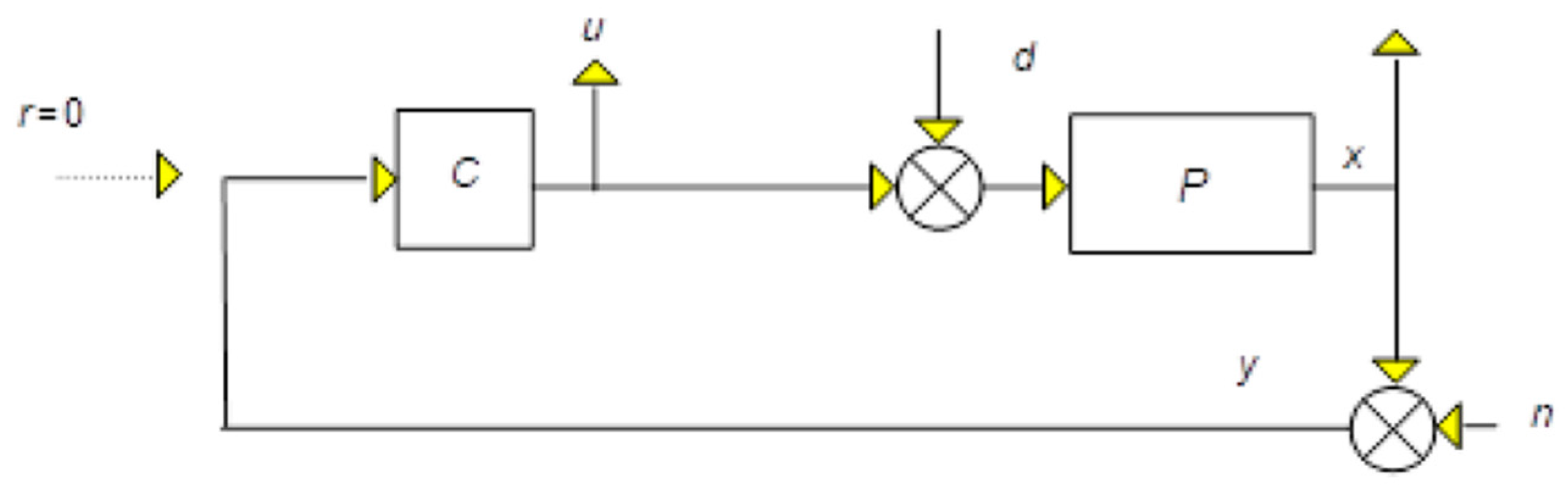
2.1. Frequency Domain

In a transfer function matrix, the structured singular value is defined as,

$$\mu (M)=\{\begin{array}{c}\frac{1}{\underset{k_m}{\min }\{\det (I-k_{m}M\mathsf{\Delta })=0,\begin{array}{c}\overline{\sigma }(\mathsf{\Delta })\le 1\}\end{array}}\\ 0,\mathrm{if} \mathrm{no} \mathrm{such} \mathrm{structured} \mathrm{exists}\end{array}$$

(6)

This matrix specifies the smallest structured Δ and has $\overline{\sigma }\left(\mathsf{\Delta }\right)$ as a function (sigma is the structured singular value for the uncertainty modeling), and, as a result, the determinant becomes zero, i.e., det(I − MΔ) = 0: then $\mu \left({\rm M}\right)=1/\overline{\sigma }\left(\mathsf{\Delta }\right)$. Equation (6) calculates the singular value. The upper and lower limits are visually presented and they should be less than one (1) for the specific Kp (arithmetic parameter for the stiffness matrix) and Km (arithmetic parameter for the scaled mass matrix) values. Following this, it is desired that the μ values are lower than 1, as shown in the results section. The principle followed was the smaller, the better [15,16,17].

2.2. Design Objectives

Design goals can be divided into two groups:

Nominal performance

• Small control effort.
• Attenuation of disturbances with acceptable transient characteristics (overshoot, settling time).
• Strength of closed loop system (plant + controller).

Robust performance

4.

The above criteria (1)–(3) should be satisfied even when noise exists in the modeling procedure.

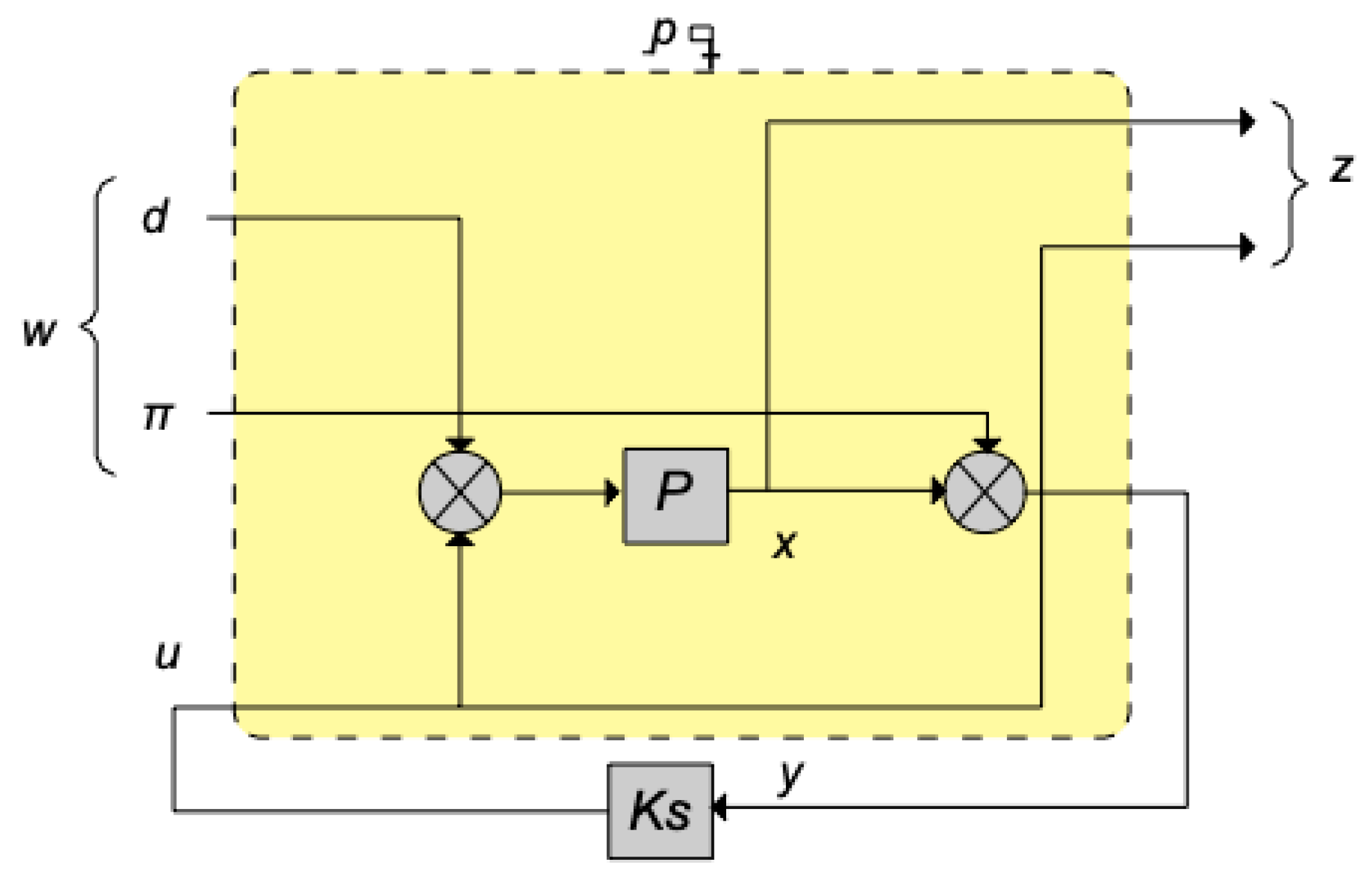
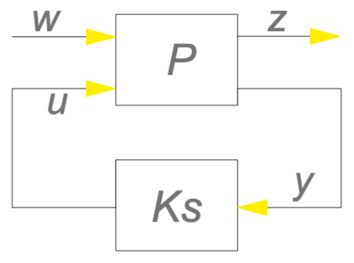
2.3. System Specifications

To obtain the necessary system specifications, the system should be represented in the (N, Δ) structure to achieve the aforementioned objectives. The conventional diagram is depicted in Figure 2.

The disturbance vector (mechanical force) d and noise vector n are the diagram’s two inputs, and the control vector u and state vector x are the diagram’s two outputs. It is expected in what follows that,

$${\Vert \begin{array}{c}d\\ n\end{array}\Vert }_2\le 1,\begin{array}{c}\end{array}{\Vert \begin{array}{c}u\\ x\end{array}\Vert }_2\le 1$$

(7)

If that is not the case, then the original signals can be modified using the right frequency-dependent weights to give the altered signals this feature [9,13].

Rewrite Figure 2 similarly to Figure 3:

Or with fewer details (Figure 4),

with,

$$z=\left[\begin{array}{c}u\\ x\end{array}\right],\begin{array}{c}\end{array}w=\left[\begin{array}{c}d\\ n\end{array}\right]$$

(8)

where z is the output (control vector u, and the state vector x) controllable variables as well as exogenous inputs (mechanical disturbances vector and the noise) [12,14,18]. Given that P is composed of two inputs and two outputs, it is typically partitioned as follows,

$$\left[\begin{array}{c}z(s)\\ y(s)\end{array}\right]=\left[\begin{array}{cc}{P}_{zw}(s)& P_{zu}(s)\\ P_{yw}(s)& P_{yu}(s)\end{array}\right]\left[\begin{array}{c}w(s)\\ u(s)\end{array}\right]\stackrel{\mathsf{o}\mathsf{\rho }}{=}P(s)\left[\begin{array}{c}w(s)\\ u(s)\end{array}\right]$$

(9)

Also,

u(s) = K_s(s)y(s)

(10)

The transfer function for a closed loop is obtained by substituting (10) in (9) N_zw(s) with K_s(s) the controller of our system,

N_zw(s)=P_zw(s)+P_zu(s)K_s(s)(I − P_yu(s)K_s(s))⁻¹P_yw(s)

(11)

To determine robustness prerequisites, an additional graph is needed, as shown in Figure 5:

where the N factor is defined by Equation (11) and the uncertainty parameter, which is modeled in Δ, should satisfy the following criterion ║Δ║∞ ≤ 1 (details later). Where

z = $ℱ$_u(N, Δ)w = [N₂₂ + N₂₁Δ(I − N₁₁Δ)⁻¹N₁₂]w = Fw

(12)

We can state the following definitions based on this structure, shown in

Table 2. Definitions.

Nominal stability (NS) ⇔	N internally stable
Nominal performance (NP) ⇔	║N22(jω)║∞ < 1, ∀ω and NS
Robust stability (RS) ⇔	F = Φu(N, Δ) stable ∀Δ, ║Δ║∞ < 1 and NS
Robust performance (RP) ⇔	║F║∞ < 1, ∀Δ, ║Δ║∞ < 1 and NS

:

The following conditions are demonstrated to be true for real or complex block-diagonal perturbations Δ:

I.

If M is internally stable, the system is presumably stable;

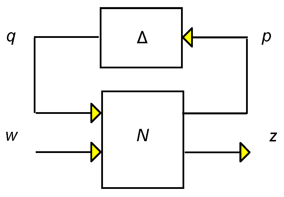
II.

If the system performs about average;

III.

If and only if, the system (M, Δ) is robustly stable,

$$\underset{\omega \in ℝ}{\sup }{\mu }_{\mathsf{\Delta }}\left(N_{11}(\mathrm{j}\omega )\right)<1$$

(13)

where the structured singular value of N is the parameter μ_Δ in the criterion, for the structured uncertainty set Δ. This condition is known as the generalized small gain theorem [12,13,14].

IV.

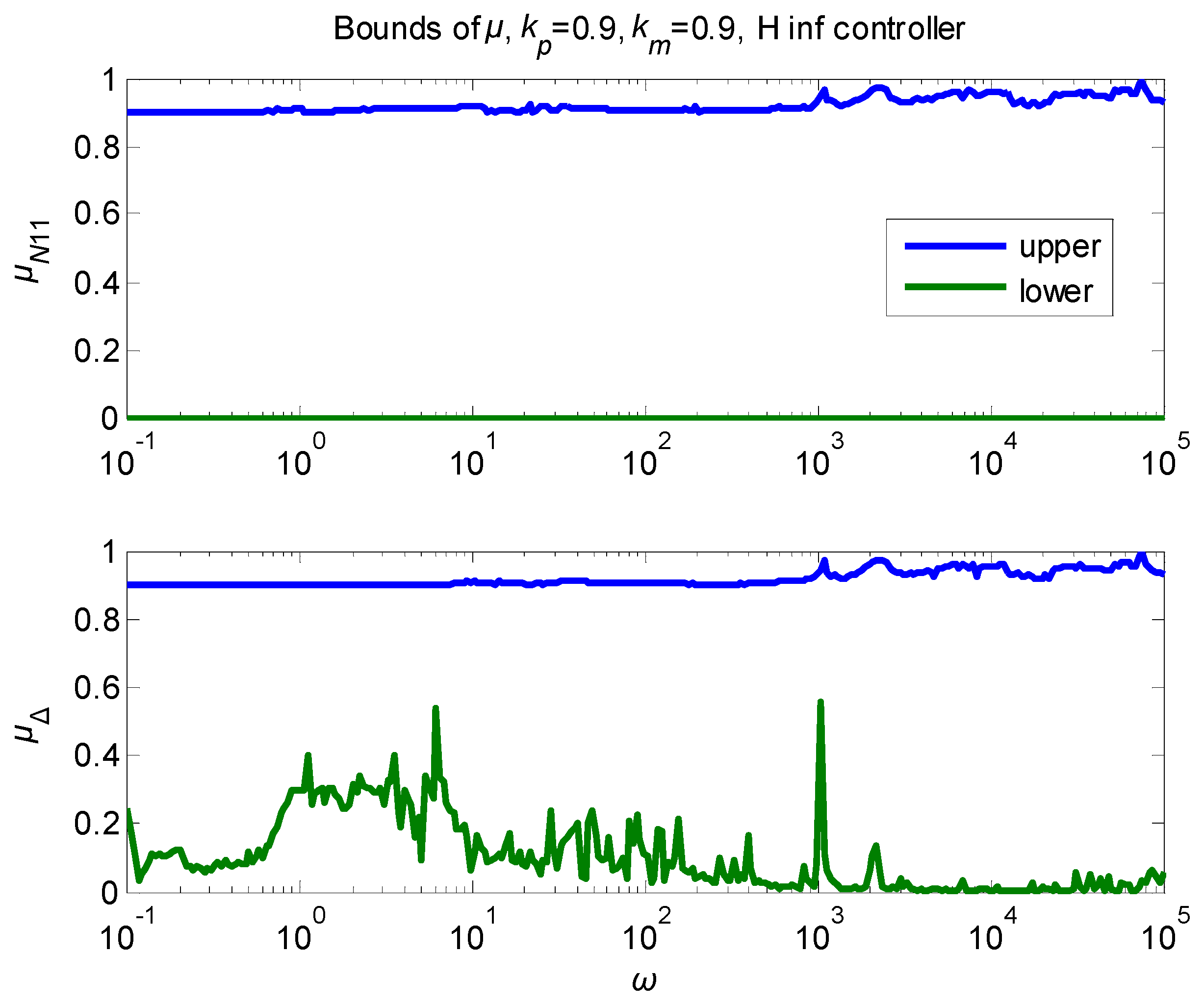
The system (N, Δ) exhibits robust performance if and only if,

$$\underset{\omega \in ℝ}{\sup }{\mu }_{{\mathsf{\Delta }}_a}\left(N(\mathrm{j}\omega )\right)<1$$

(14)

where

$${\mathsf{\Delta }}_a=\left[\begin{array}{cc}{\mathsf{\Delta }}_p& 0\\ 0& \mathsf{\Delta }\end{array}\right]$$

(15)

and Δ_p is fully complex and has the same structure as Δ and dimensions corresponding to (w, z). Unfortunately, only bounds on μ can be estimated [19,20].

2.4. Controller Synthesis

All the aforementioned provide solutions to analytical problems and methods for evaluating and contrasting controller performance. A controller that provides a specific performance in terms of the structured singular value may be calculated [12,13].

This is the so-called (D, G-K) iteration [9], in which finding a μ-optimal controller K_s such that μ(Φ_u(F(jω)), K_s(jω)) ≤ β, $\forall$ω, is transformed into the problem of finding transfer function matrices D(ω) $ϵ\forall \mathsf{\Delta }$ and G(ω) ϵ Γ, such that,

$$\underset{\omega }{\sup }\overline{\sigma }\left[\left(\frac{D(\omega )({\mathrm{F}}_u\left(F(j\omega ),{\mathrm{K}}_s(j\omega )\right)D^{-1}(\omega )}{\gamma }-\mathrm{j}G(\omega )\right){\left({\rm I}+G^2(\omega )\right)}^{-\frac{1}{2}}\right]\le 1,\begin{array}{c}\forall \omega \end{array}$$

(16)

Unfortunately, even discovering local maxima is not guaranteed by this approach; however, a technique known as D-K iteration is available for complex perturbations (also implemented in MATLAB) [12,13,16]. It combines H_inf synthesis and μ-analysis and often produces positive results. An upper limit on μ in terms of the scaled single value serves as the starting point,

$$\mu (N)\le \underset{D\in 𝒟}{\min }\overline{\sigma }(DN{D}^{-1})$$

(17)

It is aimed to determine the controller, which lowers the peak over frequency of its upper limit,

$$\underset{K}{min}\left(\underset{D\in \Delta }{min}\parallel DN\left(K_s\right)D^{-1}{\parallel }_{\infty }\right)$$

(18)

by alternating between minimizing ${\Vert DN(K_s)D^{-1}\Vert }_{\infty }$ with respect to either K_s or D (while maintaining the other constant) [9].

3. Results and Discussion

Through the relation, the function f_m(t) was produced from the wind velocity data.

$$f_m(t)=\frac{1}{2}\rho C{}_{u}V^2(t)$$

(19)

where V = velocity, ρ = density, and C_u = 1.2.

On one side of the structure, every node is subjected to periodic sinusoidal loading pressure that simulates a severe wind.

The boundaries on the values in the frequency domain are displayed in Figure 6. This results in a deviation of the mass and stiffness matrices M, and K of about 90% from their nominal values.

As can be seen, the system is still stable and performs robustly, because, for all relevant frequencies, the upper bounds of both values remain below 1.

Additionally, we regulate the structure in the state space domain by varying the nominal values of the matrices A and B, stiffness matrix K, and mass matrix M(rel.4). Account factors are considered, such as nonlinearities and system dynamics that the modeling procedure neglects, an insufficient understanding of disturbances, the disturbances caused by the environment’s effect, and the decreased accuracy of system sensor data.

The results, as shown in Figure 7, are excellent: oscillations were suppressed even for varying prices of the system’s primary matrices A and B; additionally, the oscillations were reduced by differentiating the costs of the mass and stiffness matrices (12) and preserving the piezoelectric components’ voltages within their endurance ranges. Figure 7 and Figure 8 show the displacement of the free end of the smart structure when applying H_infinity control (close loop with PZTvoltages)in the schematic with the blue line. The smart piezoelectric structure almost has no vibrations, and it maintains equilibrium even when the key system matrices (A, B, M, and K) have different prices. In Figure 7 with green, red, light blue and petrol line we can see the displacement of the free end of the beam with different prices of matrices A and B of our system for the open loop that means without PZT voltages. Also in Figure 8 with green, red, light blue and petrol line we can see the displacement of the free end of the beam with different prices of matrices M and K of our system for the open loop that means without PZT voltages. Figure 7 and Figure 8 in the last graph show the changes when the PZT material properties change. The smart piezoelectric structure almost has no vibrations, and it maintains equilibrium even when the key system matrices (A, B, M, and K) have different prices. The initial parameters are the mass, the damping, and the stiffness matrix. In Figure 7 and Figure 8 these parameters change for the open and the closed loop—this means without PZT material and with PZT material. This work focuses on a specific PZT material with its properties shown in Table 1. Figure 7 (last graph) shows the changes when the PZT material properties change.

The discovered H_infinity controller is 24 in order. Numerous scientists have proposed algorithms for order reduction as a result of the fact that the order of the controller, which is equal to the order of the system, is substantially higher than the order of conventional controllers such as PI and LQR. The following process will use the most widely used of these algorithms, known as Hifoo [21], which has been implemented in the Matlab environment. The main issue is to calculate a reduced-order n < 24 controller that preserves the performance of the H_infinity criterion and the behavior of a full-order controller of the given system. As a mechanical input to this controller, 10 KN is taken at the free end of the structure. In Figure 9 we can see the beam-free end displacement with and without control, using Hifoo recovery time 0.05 sec (0.03 with H_infinity), the steady-state error of the order of 10⁻⁵ m (10⁻⁶ with H_infinity) maximum elevation 2.1 × 10⁻⁴ (0.3 × 10⁻⁴ with H_infinity) and vibration suppression at 90% (98% with H_infinity). In Figure 10, we can see the voltages within the piezoelectric limits of 30 volts.

The frequency response of the weighting function and matching model is shown in Figure 11. The graph of the function remains below unity so the controller archives robust performance for the given data.

4. Conclusions

The ability of piezoelectric materials to directly transform mechanical energy into electrical energy and vice versa has made them the most desirable functional materials for sensors and actuators in smart constructions. They exhibit outstanding frequency responsiveness and electromechanical coupling properties. In this study, we include active vibration suppression and robust control in the dynamics of a clever piezoelectric system. By using the established vibration control methods on a clever piezoelectric construction, numerical evaluations are performed and analyzed in order to confirm the efficiency of the method. We include modeling uncertainties by accounting for the nonlinearity of the system that was not taken into account in the model, our incomplete understanding of the model’s values and parameters, and their physiological fluctuations during the duration of the structures’ operation. An H_infinity-based controller is designed to suppress the vibration of the smart piezoelectric structure under dynamical loading. The robustness of the H_infinity controller to parametric uncertainty in vibration suppuration problems is shown. The benefit of robust control and active vibration suppression in the dynamics of smart structures is amply illustrated by this work. H_infinity control has certain advantages for the analysis of robust control systems. Unfortunately, relatively complicated modeling and resulting controllers lead to restricted practical applications. These drawbacks will be gradually eliminated due to the availability of cheaper and more powerful electronic components for control implementation. Future research will be focused on experimental verification in this direction.

References

1. Bandyopadhyay, B.; Manjunath, T.C.; Unapathy, M. Modeling, Control, and Implementation of Smart Structures; Springer: Berlin, Heidelberg, Germany, 2007; ISBN 10 3-540-48393-4. [Google Scholar]
2. Burke, J.V.; Henron, D.; Kewis, A.S.; Overton, M.L. Stabilization via Nonsmooth, Non-convex Optimization. IEEE Trans. Autom. Control 2006, 5, 1760–1769. [Google Scholar]
3. Doyle, J.C.; Glover, K.; Khargoneker, P.; Francis, B. State space solutions to standard H2 and H∞ control problems. In Proceedings of the 1988 American Control Conference, Atlanta, GA, USA, 15–17 June 1988; Volume 34, pp. 831–847. [Google Scholar]
4. Francis, B.A. A Course on H∞ Control Theory; Springer: Berlin, Heidelberg, Germany, 1987. [Google Scholar]
5. Friedman, J.; Kosmatka, K. An improved two node Timoshenko beam finite element. J. Comput. Struct. 1993, 47, 473–481. [Google Scholar]
6. Kimura, H. Robust stability for a class of transfer functions. IEEE Trans. Autom. Control 1984, 29, 788–793. [Google Scholar]
7. Miara, B.; Stavroulakis, G.; Valente, V. Topics on Mathematics for Smart Systems, Proceedings of the European Conference, Rome, Italy, 26–28 October 2006; World Scientific Publishers: Singapore, 2007. [Google Scholar]
8. Moutsopoulou, A.; Pouliezos, A.; Stavroulakis, G.E. Modelling with Uncertainty and Robust Control of Smart Beams. Paper 35, Proceedings of the Ninth International Conference on Computational Structures Technology, Athens, Greece, 2–5 September 2008; Topping, B.H.V., Papa-drakakis, M., Eds.; Civil Comp Press: Edinburgh, UK, 2008. [Google Scholar]
9. Yang, S.M.; Lee, Y.J. Optimization of non collocated sensor, actuator location and feedback gain and control systems. Smart Mater. Struct. J. 1993, 8, 96–102. [Google Scholar]
10. Chandrashekara, K.; Varadarajan, S. Adaptive shape control of composite beams with piezoelectric actuators. Intell. Mater. Syst. Struct. 1997, 8, 112–124. [Google Scholar]
11. Lim, Y.H.; Gopinathan, V.S.; Varadhan, V.V.; Varadan, K.V. Finite element simulation of smart structures using an optimal output feedback controller for vibration and noise control. Int. J. Smart Mater. Struct. 1999, 8, 324–337. [Google Scholar]
12. Zhang, N.; Kirpitchenko, I. Modelling dynamics of a continuous structure with a piezoelectric sensor/actuator for passive structural control. J. Sound Vib. 2002, 249, 251–261. [Google Scholar]
13. Zhang, X.; Shao, C.; Li, S.; Xu, D. Robust H∞ vibration control for flexible linkage mechanism systems with piezoelectric sensors and actuators. J. Sound Vib. 2001, 243, 145–155. [Google Scholar] [CrossRef]
14. Kwakernaak, H. Robust control and H∞ optimization. Tutor. Hper JFAC Autom. 1993, 29, 255–273. [Google Scholar]
15. Stavroulakis, G.E.; Foutsitzi, G.; Hadjigeorgiou, E.; Marinova, D.; Baniotopoulos, C.C. Design and robust optimal control of smart beams with application on vibrations suppression. Adv. Eng. Softw. 2005, 36, 806–813. [Google Scholar] [CrossRef]
16. Packard, A.; Doyle, J.; Balas, G. Linear, multivariable robust control with a μ perspective. ASME J. Dyn. Syst. Meas. Control 50th Anniv. Issue 1993, 115, 310–319. [Google Scholar] [CrossRef]
17. Tiersten, H.F. Linear Piezoelectric Plate Vibrations; Plenum Press: New York, NY, USA, 1969. [Google Scholar]
18. Zames, G. Feedback minimax sensitivity and optimal robustness. IEEE Trans. Autom. Control 1993, 28, 585–601. [Google Scholar] [CrossRef]
19. Chen, B.M. Robust and Hinf Control; Springer: London, UK, 2000. [Google Scholar]
20. Iorga, L.; Baruh, H.; Ursu, I. A Review of H∞ Robust Control of Piezoelectric Smart Structures. ASME. Appl. Mech. Rev. 2008, 61, 040802. [Google Scholar] [CrossRef]
21. Millston, M. HIFOO 1.5: Structured Control of Linear Systems with a Non-Trivial Feedthrough. Master’s Thesis, Courant Institute of Mathematical Sciences, New York University, New York, NY, USA, 2006. [Google Scholar]
Figure 1. (a) Piezoelectric smart beam; (b) Piezoelectric smart cantilever beam.
Inventions 08 00047 g001
Figure 2. Typical control block graph.
Inventions 08 00047 g002
Figure 3. Two-port detailed graph.
Inventions 08 00047 g003
Figure 4. Two-port graph.
Inventions 08 00047 g004
Figure 5. Uncertainty modeling N-Δ structure.
Inventions 08 00047 g005
Figure 6. Bounds of the μ value.
Inventions 08 00047 g006
Figure 7. Results for matrices A and B with and without Hinf, controlling for sinusoidal external inputs, at various prices.
Inventions 08 00047 g007
Figure 8. Results for matrices M (mass) and K (stiffness) at various costs, both with and without Hinf control of the external sinusoidal inputs.
Inventions 08 00047 g008
Figure 9. Displacement of the free end of the structure with and without Hifoo.
Inventions 08 00047 g009
Figure 10. Piezoelectric voltages with reduced order controller for the first four nodes.
Inventions 08 00047 g010
Figure 11. The robust performance criterion measure.
Inventions 08 00047 g011