Article

Reduction in the Computational Complexity of Calculating Losses on Eddy Currents in a Hydrogen Fuel Cell Using the Finite Element Analysis

Research Institute of Electromechanics, Platov South-Russian State Polytechnic University (NPI), Prosveshcheniya Str. 132, 346428 Novocherkassk, Russia
*
Author to whom correspondence should be addressed.
Inventions 2023, 8(1), 38; https://doi.org/10.3390/inventions8010038
Submission received: 20 December 2022 / Revised: 25 January 2023 / Accepted: 28 January 2023 / Published: 1 February 2023
(This article belongs to the Special Issue Data Analytics in the Energy Sector)

Abstract

:
This paper considers the issues of the reduction in the computational complexity of the numerical problem and the requirements of the computer memory size when calculating the power of the eddy currents in a hydrogen fuel cell based on a proton exchange membrane. The study was performed on a model problem based on a geometric pattern of a hydrogen fuel cell of typical dimensions and characteristics operating at a nominal load in steady-state conditions. The power of the eddy currents was calculated using a numerical model based on a tetrahedral finite element mesh and a mathematical model of a quasi-stationary electromagnetic field in the classical formulation through the vector magnetic potential. The requirements for the minimum degree of the geometric model approximation by a finite element mesh to achieve mesh stability of the computational problem results were defined. The paper considers issues of finite element order selection, the method of ordering, and the solution of the systems of linear algebraic equations (SLAEs). It shows the techniques for determining the accuracy of the calculated SLAE solution obtained by the direct method, as well as the effectiveness of the low-rank approximation of the SLAE to reduce the computational complexity of the computational problem solution and reduce the requirements for the amount of computer memory needed, considering the reduced accuracy of the SLAE solutions.

1. Introduction

In the literature, the issue of eddy current occurrence in fuel cells has been considered, as a rule, in terms of ways to control the integrity and homogeneity of the cell structure [1,2]. The calculation of eddy current losses in fuel cells during their operation has not been considered. Traditionally, only the activation losses between the anode and the cathode, as well as ohmic losses in the electrolyte and membrane, are considered [3,4,5]. The calculation of eddy current power values is possible, for example, through the analytical method, some numerical methods, and the finite element method. The analytical method based on the substitution scheme was considered in [6], but it was characterized by high complexity in the preparation of the initial data. The application of the finite element method is complicated by the design features of the fuel cell: its electrodes and proton exchange membrane have a large area and small thickness (usually 0.12–0.8 mm), which leads to the need to use finite elements with small values of the characteristic length. This in turn results in the creation of a large finite element mesh and high computational complexity. In this work, for the first time (applied to fuel cells), methods for reducing the computational complexity of the process of calculating the power of eddy currents using the finite element method were considered by determining the minimum allowable degree of finite element approximation of the geometric model and by the choice of the numerical solver’s configuration and the methods of solving the SLAE.

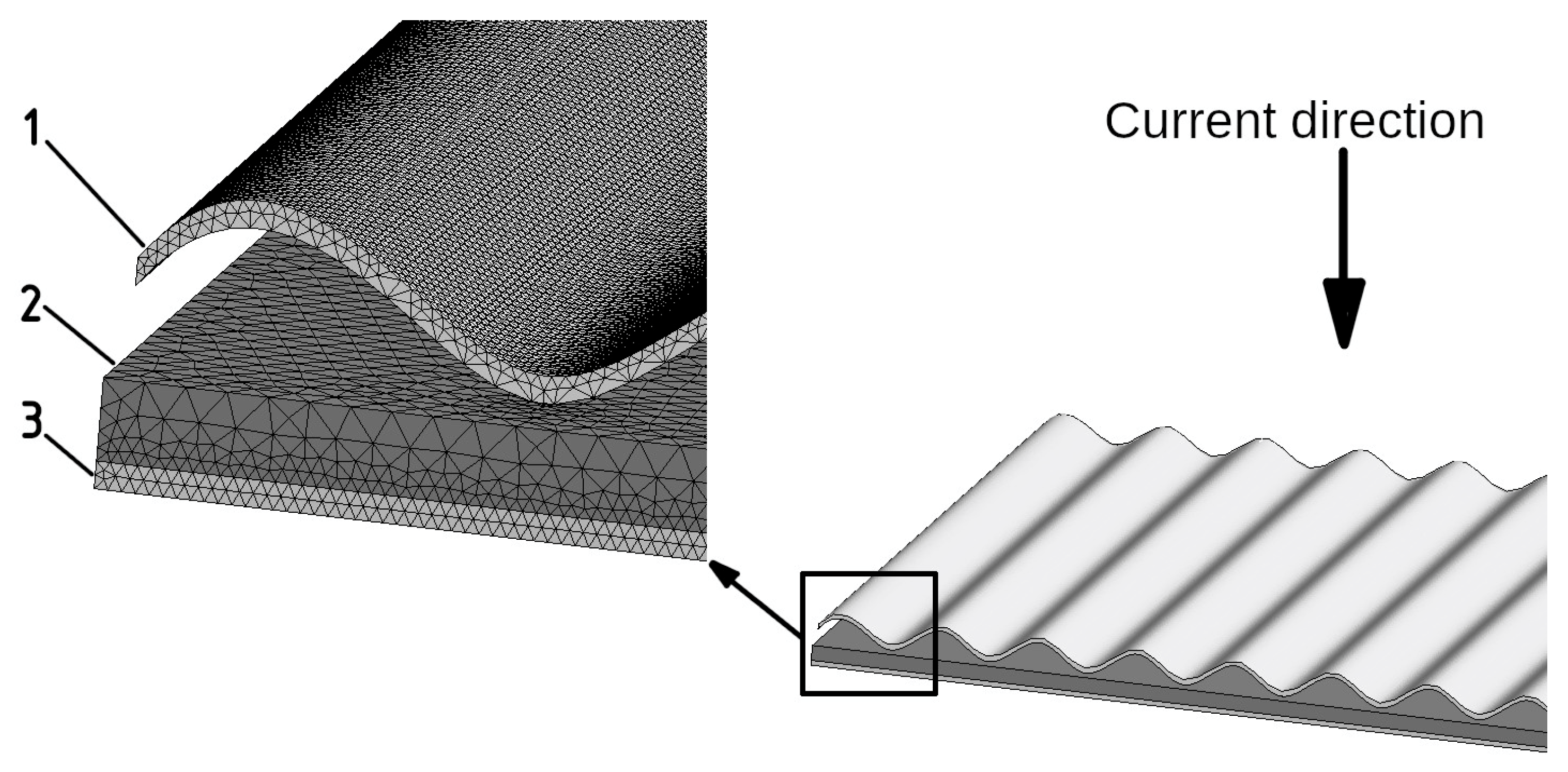
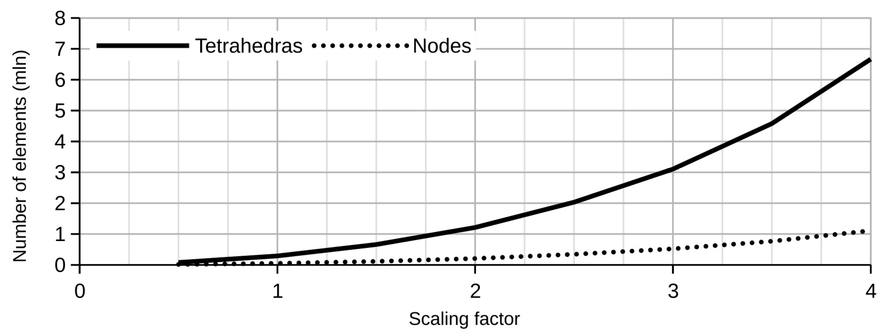
2. Geometric and Finite Element Models

The computational domain was limited to a sphere with a radius of 0.2 m. It included models of the fuel cell parts: the anode, cathode, and proton exchange membrane. The thickness of the titanium electrodes was 0.16 mm, and of the membrane was 0.56 mm. The length and width of the fuel cell were 230 mm and 50 mm, respectively. The corrugated electrode had a pitch of wave of 4 mm and a wave height of 2 mm (Figure 1). The geometric and finite element models of all the computational model problems were created in the Gmsh environment (version 4.10.4, compiled from source code; C. Geuzaine and J.-F. Remacle, Belgium [7]). The geometric models were created using the geometric modeling kernel OpenCASCADE Core Technology, the finite element mesh of R2 space objects was generated using the MeshAdapt algorithm [8], and the finite element mesh of the R3 space objects was generated using the HXT algorithm [9].
The finite element mesh, depending on the basic characteristic lengths of the finite element edges of the fuel cell (from 0.04 mm to 0.32 mm), contained 0.014–1.1 million nodes and 0.08–6.67 million tetrahedrons. The basic values of the characteristic lengths were the ratios of the electrode thickness to the scaling factor (the factor showed how many times less the characteristic length was than the electrode thickness in the range of 0.5 to 4).
The choice of the values of the range of scaling factors was determined on the basis of the need to provide both a knowingly insufficient and potentially excessive degree of approximation of the conductive domain to determine the mesh-related stability of the calculation result of the eddy currents’ power [10]. It should be highlighted that the HXT algorithm has built-in means to optimize finite elements according to quality criteria that provide high minimum and average values of the quality indicators. Finite elements have a quality not worse than 0.06 (average value: 0.74) by the Gamma criterion [11]. The dependence of the number of nodes and tetrahedrons in the finite element mesh on the scaling factor is shown in Figure 2.

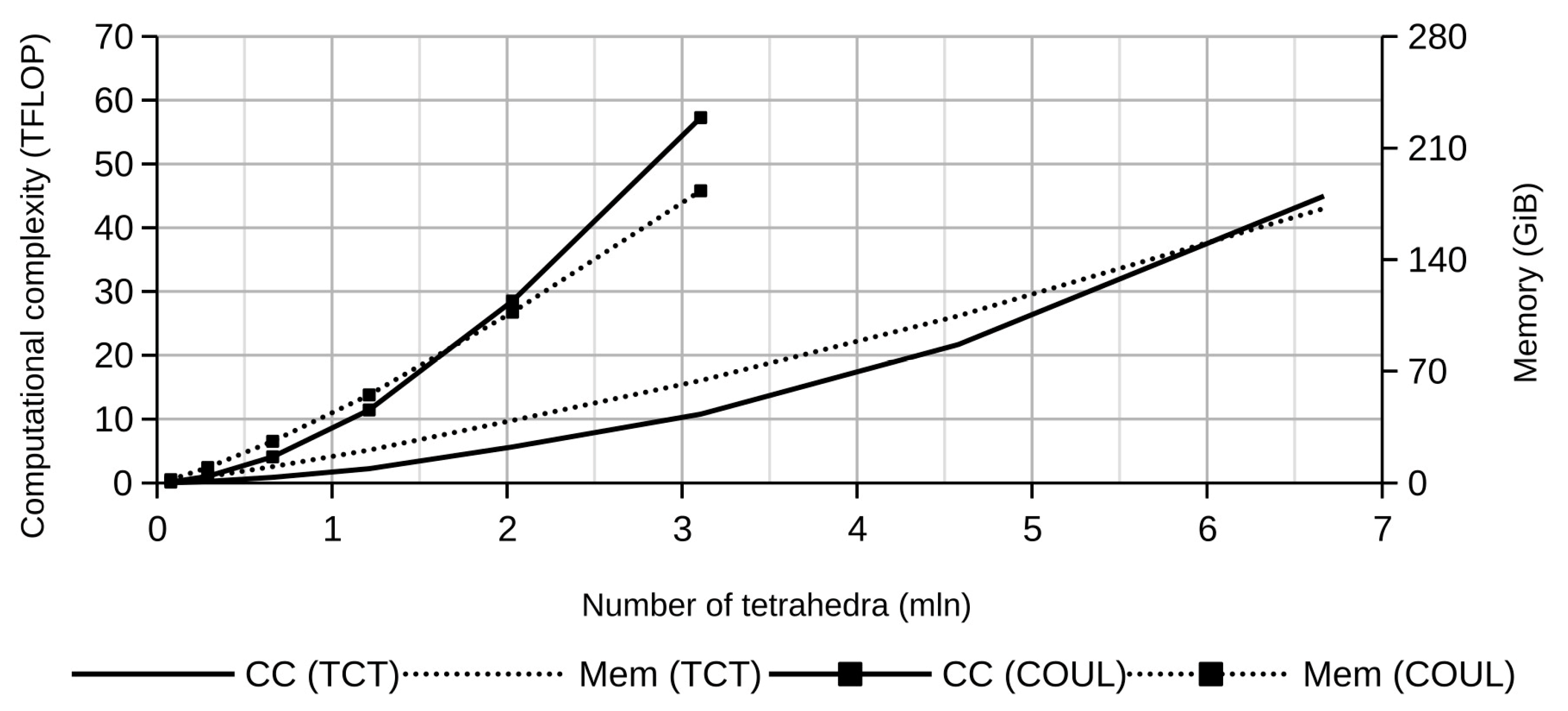
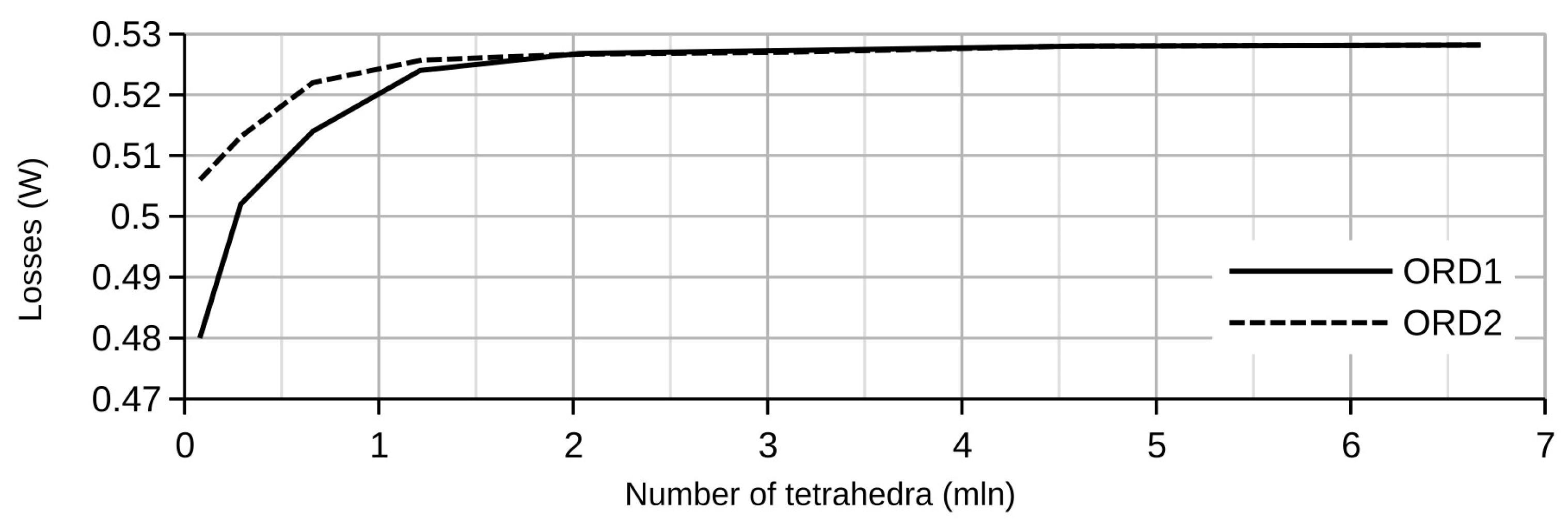
3. Mathematical Model

We used an environment for treating discrete numerical problems called GetDP (version 3.4.1, compiled from source code; P. Dular and C. Geuzaine, University of Liège, Liège, Belgium [12]) to solve the computational problem. The GetDP environment does not contain ready-made implementations of mathematical models of any physical processes or related constructions (functional spaces and sets of basis functions, descriptions of methods of integration over the finite element domain, or methods of primary mathematical processing), but it contains wide function sets for the design of these constructions. Therefore, for numerical simulation a description of the mathematical model of the electromagnetic field in the weak A-V formulation (vector magnetic potential) in the form of the Petrov–Galerkin equations [13] was developed on the basis of the finite element model considered above, and of the classical model of the vector magnetic potential of the electromagnetic field [14]:
(rotA/μ, rotA′)Ω − (JS, A′)ΩS + (n × HS, A′)ΓΩ = 0,
(A·w)Ω = 0, ΓΩ ∉ Ω,
(∇·A)ΓΩ = 0,
where μ is a magnetic permeability, n × HS are Neumann boundary conditions along the boundaries ΓΩ, Ω is a computational domain, and w is a vector field that has no closed lines (applied to the cotree elements).
In the model used, the desired value is a value of the vector magnetic potential on the edges of the finite elements, which requires a description of the edge-based functional space. Expressions (2) and (3) are, respectively, the tree–cotree and Coulomb gauge conditions to ensure the uniqueness of the magnetic vector potential. If the Coulomb gauging condition is used, it is necessary to additionally introduce a nodal functional space. Since the problem considered is quasi-stationary, expression (1) was supplemented with non-stationary components in the following form:
(rotA/μ, rotA′)Ω − (JS, A′)ΩS + (n × HS, A′)ΓΩ + (σ∂tA, A′)Ωσ + (σgradV, A′)Ωσ = 0,
(σ∂tA, gradV′)Ωσ + (σgradV, gradV′)Ωσ = ∑ IiUi(V′),
where Ωσ is a volume domain of electrically conductive materials, V is a scalar field potential within the domain functional space Ωσ, σ is an electrical conductivity, and Ii and Ui are the current and voltage in each unit circuit of a massive conductor (in this case, the conductive volume domain).
The formulation used for the mathematical model was based on a model that was described in detail in [15]. The above expression does not contain the angular frequency ω typical for the classical A-V statement of the vector magnetic potential in the frequency domain, and some components of the Galerkin–Petrov equations (weight functions and other), because their determination was performed by internal functions of the GetDP environment, in accordance with the description of the functional spaces and properties of the numerical problem. The electrical conductivity of the titanium electrode material was 1.72 MS/m, and the proton exchange membrane was 61 S/m. Under the normal usage conditions of a fuel cell in a stack (battery of fuel cells), the current flow from one cell to another occurs through the entire contact area of electrodes of neighboring cells and within one cell through the contact area of the electrode and proton exchange membrane. Since the steady-state operation of the fuel cell at nominal power was considered, the current value 26 A was given by the set of current density vectors through the contact area of the electrode with the electrode of the adjacent cell. For the flat electrode, the current density was 2260 A/m2, and for the corrugated electrode, it was 30,500 A/m2 (conductive pad size 0.3 × 50 mm, 57 conductive pads per electrode). In the finite element mesh and mathematical model for the domains of conducting bodies, thin layers (boundary layers) were not distinguished since the electrode thickness of 0.16 mm did not exceed half the depth of the skin effect [16], 0.396 mm, at a frequency of 100 kHz.
In contrast to expressions (2) and (3), for a quasi-stationary electromagnetic field, both variants of the gauge conditions applied exclusively to the environment domain Ωe or domain boundaries of the computational domain Ω without considering the common boundaries with the domain of the conducting materials Ωσ:
(∇·A)ΓΩ = 0, (A·w)Ωe = 0, ΓΩσ ∉ Ωe,
(∇·A)ΓΩ = 0, (ΓΩσ, Ωσ) ∉ Ω.
Additionally, a gauge condition was applied to determine the zero voltage potential on the surfaces of the domain of the electrically conductive materials Ωσ, for which an additional nodal functional space was introduced:
(Ur)ΓΩσ = 0,
where Ur is the voltage potential, and ΓΩσ are the boundaries of the domain of conductive materials.
The power of the eddy currents in the considered problem was calculated at the stage of post-processing (primary mathematical processing) in the GetDP environment according to the following expression:
P = ∫σ‖∂tA + dgradV2.
The mathematical model of the electromagnetic field and the methods for preparing and solving the computational problems with the Gmsh and GetDP environments were previously verified in [17]. The GetDP environment is configured to work with the PETSc toolkit (version 3.16.6, compiled from source code; Argonne National Laboratory, Lemont, IL, USA [18]) using both a third-party problem solver (MUMPS, version 5.4.0, compiled from source code via PETSc toolkit; Mumps Technologies SAS, Lyon, France [19]; solution of the SLAE by the LU factorization method) and a built-in problem solver (iterative methods of the Krylov subspace) to solve the computational problems. To order the elements of the SLAE matrices when working with the MUMPS problem solver, the SCOTCH (version 5.1, compiled from source code via PETSc toolkit; LaBRI of l’Université de Bordeaux, Talence, France [20]) and PORD (version 1.0, compiled from source code via PETSc toolkit; Jürgen Schulze, Universität Paderborn, Paderborn, Germany [21]) methods were used. The simulation was performed on a PC with 32 GB of RAM (16.4 GB/s bandwidth), 256 GB of storage (buffered NVMe solid-state drive with read and write speeds of up to 1.6 GB/s), and a six-core CPU with a peak performance of 112 GFLOPs in double precision of floating point arithmetic with FMA4 and AVX instruction sets.
Thus, the formation and solution of the numerical problem proceeded as follows: geometric and finite element models were created in the Gmsh environment, after which the finite element mesh, along with the description of the mathematical model and the scenario for solving the numerical problem, were transferred to the GetDP environment. GetDP performed preprocessing and transferred the generated SLAE to the MUMPS solver through the interface of the PETSC toolkit. Inside the solver, the ordering, preconditioning, and solving of the SLAE were performed. The solution result was returned to the GetDP, where post-processing was performed for the convenience of the subsequent interpretation of the results.
For the problem considered, we investigated the dependence of computational complexity on the number of elements in the mesh for both variants of the problem formulation: with tree–cotree and Coulomb gauge conditions (Figure 3). The SLAE was solved by the LU factorization method, and the ordering was realized using the SCOTCH method.
We highlight that the computational complexity of the numerical problem with Coulomb gauge condition was 4.5–5.5 times higher than that in the case with the tree–cotree gauge condition, and the required memory size were also significantly higher, in 3–3.5 times. Thus, with 3.1 million tetrahedrons already, the entire amount of available memory was used even for the Out-Of-Core mode (most of the solution kernel was taken from RAM to storage), and for computational problems based on meshes of larger sizes, the study was not performed. At the same time, such a gauging does not give any advantages in the calculation of eddy current losses, and it will not be used in further studies.
The study of mesh-related stability showed that in the case of using the first-order elements (designation “ORD1” on the schedules) with characteristic lengths of less than 0.5 of the electrode thickness, i.e., 0.08 mm, did not lead to a significant change in the calculated value of eddy current losses (Figure 4). This value of the finite elements characteristic length led to the generation of a mesh with 1.21 million tetrahedrons. At the same time, the use of second-order finite elements (designation “ORD2”) ensured the calculation of eddy current losses with sufficient accuracy when the value of the characteristic length was less than 2/3 of the electrode thickness (0.66 million tetrahedrons). The power value of the eddy current losses obtained with the model considered was 0.527 W (0.523 W for a second-order mesh with 0.66 million tetrahedrons).
Using the built-in PETSc and MUMPS tools, we investigated the computational complexity and evaluated the accuracy of solving the numerical problem (SLAE) for two configurations of the problem solver: using arithmetic double-precision real numbers and double-precision complex numbers (Figure 5). The SLAE was solved by the LU factorization method, and the ordering was realized using the SCOTCH method. It was found that the arithmetic’s application of complex numbers instead of real numbers allowed a decrease in the computational complexity manifold (by 7–8 times for all investigated meshes of finite elements) and the requirements for the computer memory size (by 1.85–1.95 times). It should be noted that the difference in computational complexity of numeral problems based on first- and second-order finite element meshes was insignificant, as was the difference in the required amount of computer memory.
There are several generally similar approaches [22,23,24], which use eigenvalues and condition numbers to calculate the relative error of the calculated solution, to evaluate the accuracy of the calculated SLAE solution by the direct method. However, it should be considered that depending on the basis of the norm and the characteristics of the SLAE, the obtained values of the expected accuracy can be quite far from the real values. For example, [25,26] have shown that although eigenvalues are convenient for the calculation of matrix condition numbers, their blind usage can lead to incorrect conclusions since even for poorly conditioned or large systems, it is possible to obtain a unit value of the condition number based on any of the standard norms. It can be noted that the Manhattan and spectral condition numbers (1- and 2-norm, respectively) can take unit values depending on not only the formulation of the problem (the presence and type of the gauge condition) but also the number of finite elements in mesh on which the problem is based [25]. At the same time, the condition numbers for both norms cannot take a unit value simultaneously. Therefore, the usage of the relative forward error based on the component-wise relative backward errors ϖ1 and ϖ2 [22], which are computed on the basis of the scaled residual ϖ1i and ϖ2i, is a reliable way to evaluate the accuracy of the computed solution:
ϖ1i = |bAx|i/(|b| + |A| |x|)i,
ϖ2i = |bAx|i/(|A| |x|)i + ||Ai|| + ||x||,
where x is a calculated solution and Ai is a row i of the matrix A.
The scaled residual ϖ1i was calculated for all equations except those with a non-zero numerator and a small value in the denominator. The scaled residual ϖ2i was calculated for such equations. As a matter of fact, the component-wise errors ϖ1 and ϖ2 were the largest values of the scaled residuals ϖ1i and ϖ2i, i.e., the upper limit.
A technique for obtaining the value of the relative forward error based on the values of the component-wise backward errors has been shown in [22,23] and is reduced to the summation of their scaled values:
‖δx/‖xϖ1cond1 + ϖ2cond2,
where cond1 is a Manhattan condition number (1-norm) and cond2 is a spectral condition number (2-norm).
Since this approach uses two condition numbers at once, we should expect the correct calculation of the calculated solution accuracy regardless of the SLAE characteristics. Figure 6 shows the obtained values of the relative forward error of the calculated SLAE solution for different numbers of tetrahedrons in the finite element mesh. We can say that configuration of the PETSc toolkit for working with real number arithmetic instead of complex numbers led to an increase in the value of the relative forward error of the calculated SLAE solution by 6–8 orders of magnitude.
The evaluation of the calculated solution accuracy for direct methods of the SLAE solution is also necessary to reduce the time of the SLAE solution by applying BLR-factorization (low-rank approximation of SLAE) [27,28,29] without the necessity of verifying the calculation results for each numerical problem.
Comparison of the values of the relative forward error and the desired value of the target parameter of the model problem (eddy current losses) made it possible to determine an acceptable value of the error corresponding to a reliable solution to the problem. It also allowed the determination of the value of the acceptable tolerance (threshold) of the low-rank approximation for the considered problem (or group of similar problems). For example, when configuring the PETSc toolkit to use the arithmetic of double-precision complex numbers, regardless of the input parameters of the considered problem, any of its solutions with a value of the relative forward error (FERR) less than 1 × 10⁶ can be considered reliable (Figure 7; the study was performed for a computational problem based on a mesh with 1.21 million tetrahedrons).
The application of another ordering method of the matrix of unknowns (PORD instead of SCOTCH) also did not lead to a significant change in the obtained values of the relative forward error or the values of the target parameter of the problem studied. The specified value of FERR was achieved at a given tolerance of a low-rank approximation of 1 × 10⁻⁵ or less, which reduced the computational complexity of the numerical problems (in terms of CPU time utilization) by 30–40%, as was shown in [25].
Figure 8 shows the dependence of decreasing the computational complexity of the LU-factorization procedure, the required memory size, and the CPU time utilization for solving the whole numerical problem (the LU-factorization procedure was only one step in the solution of the computational problem but reached up to 90–95% of computational complexity) on the given accuracy of the low-rank approximation. As mentioned above, in this case, using an acceptable value of the tolerance of the low-rank approximation reduced the utilization of the CPU time and the requirements for the amount of necessary memory by 28–30%.
It should be noted that this paper did not consider the use of iterative methods of the Krylov subspace since the studied computational problem was built on a similar [25] mathematical model. Iterative methods for a solution of the SLAE, that based on considered computational model, are unstable or show unsatisfactory performance.

4. Conclusions

The numerical calculation of the eddy current power in the electrodes of a hydrogen fuel cell using the finite element method is complicated by the need to create a mesh in a thin body with a large area. This leads to the generation of a large mesh, and the numerical problem based on such a mesh and the mathematical models of non-stationary or quasi-stationary electromagnetic fields have high computational complexities. However, the use of second-order finite elements with the problem solver configured to work with complex number arithmetic, along with the use of low-rank approximation of matrices with a given tolerance of 1 × 10⁻⁵, allows a significant reduction in the requirements for the amount of memory and processor time utilization of the computer. In the considered case, the use of second-order finite elements, the formulation of a computational problem with the tree–cotree gauge condition, machine arithmetic of double-precision complex numbers, and BLR-factorization together allowed the fast calculation of the eddy current losses in a hydrogen fuel cell using limited hardware resources: about 10–12 GB of memory and 65–70 s of processor time. The eddy current loss value of 0.52–0.53 W obtained as a result of computer modeling was not more than 3% of the nominal power of the hydrogen fuel cell, 20.5 W. Accordingly, during the consideration of single hydrogen fuel cells, it is not an obligatory condition to take into account the power of eddy currents in steady-state operation. Such an approach to solving a numerical problem will make it possible to obtain a result in a very short time even when using a weak computer, which is especially important when performing optimization simulations and studying large-area fuel cells and even full stacks of hydrogen cells. Easily and quickly obtaining the results of eddy current power calculations can help verify and refine analytical models [30,31].

Author Contributions

Conceptualization, A.K. and A.P.; methodology, A.K. and I.V.; software, A.K. and D.B.; validation, A.K., I.V. and D.B.; formal analysis, A.P.; investigation, I.V.; resources, D.B.; data curation, A.P.; writing—original draft preparation, A.K.; writing—review and editing, A.P.; visualization, D.B.; project administration, A.P.; funding acquisition, A.P. All authors have read and agreed to the published version of the manuscript.

Funding

The manuscript is based on the results obtained during the implementation of a state assignment for the performance of scientific research on the project “Power Plants on Hydrogen Fuel Cells for Small Unmanned Vehicles: Modeling, Development, Research.” The employer is the Ministry of Science and Higher Education of the Russian Federation, research topic code FENN-2020-0022.

Data Availability Statement

Not applicable.

Conflicts of Interest

The authors declare no conflict of interest.

References

  1. Pfeif, E.; Jones, Z.; Lasseigne, A.; Koenig, K.; Krzywosz, K.; Mader, E.; Yagnik, S.; Mishra, B.; Olson, D. Submerged Eddy Current Method of Hydrogen Content Evaluation of ZIRCALOY4 Fuel Cladding. AIP Conf. Proc. 2011, 1335, 1168. [Google Scholar] [CrossRef]
  2. Felt, W. Electromagnetic Excitation Methods for Thermographic Defect Detection in Fuel Cell Materials; Technical report; National Renewable Energy Laboratory: Golden, CO, USA, 2012. [Google Scholar]
  3. Elia, G. Characterization of Voltage Loss for Proton Exchange Membrane Fuel Cell. Bachelor’s Thesis, Polytechnic University of Catalonia (UPC), Barcelona, Spain, 2015. [Google Scholar]
  4. Gou, B.; Na, W.; Diong, B. Linear and Nonlinear Models of Fuel Cell Dynamics. Dynamic Modeling and Control with Power Electronics Applications; CRC Press: Boca Raton, FL, USA, 2016. [Google Scholar]
  5. Hirschfeld, J. Tomographic Problems in the Diagnostics of Fuel Cell Stacks, PGI-1/IAS-1; Berichte des Forschungszentrums Jülich: Jülich, Germany, 2009. [Google Scholar]
  6. Burtsev, Y.A.; Pavlenko, A.V.; Vasyukov, I.V. A step-down converter of a power plant based on fuel cells for an unmanned aerial vehicle. Electr. Eng. 2021, 10, 81–85. [Google Scholar]
  7. Geuzaine, C.; Remacle, J.-F. Gmsh: A three-dimensional finite element mesh generator with built-in pre- and post-processing facilities. Int. J. Numer. Methods Eng. 2009, 79, 1309–1331. [Google Scholar] [CrossRef]
  8. Lu, Q.; Shephard, M.S.; Tendulkar, S.; Beall, M.W. Parallel mesh adaptation for high-order finite element methods with curved element geometry. Eng. Comput. 2014, 30, 271–286. [Google Scholar] [CrossRef]
  9. Marot, C.; Pellerin, J.; Remacle, J.F. One machine, one minute, three billion tetrahedra. Int. J. Numer. Methods Eng. 2018, 117, 967–990. [Google Scholar] [CrossRef]
  10. Bastos, J.; Sadowski, N. Electromagnetic Modelling by Finite Element Methods, 1st ed.; M. Dekker: New York, NY, USA, 2003. [Google Scholar]
  11. Geuzaine, C.; Remacle, J.-F. (Eds.) Gmsh Reference Manual; The documentation for Gmsh 4.8.4; Belgium, 2022. [Google Scholar]
  12. Dular, P.; Geuzaine, C.; Henrotte, F.; Legros, W. A general environment for the treatment of discrete problems and its application to the finite element method. IEEE Trans. Magn. 1998, 34, 3395–3398. [Google Scholar] [CrossRef]
  13. Biro, O.; Paul, C.; Preis, K. “The use of a reduced vector potential A-r formulation for the calculation of iron induced field errors”, ROXIE: Routine for the Optimization of Magnet X-Sections, Inverse Field Calculation and Coil End Design. In Proceedings of the First International Roxie Users Meeting and Workshop CERN, Geneva, Switzerland, 16–18 March 1998; pp. 31–47. [Google Scholar]
  14. Biro, O. Edge element formulations of eddy current problems. Comput. Methods Appl. Mech. Eng. 1999, 169, 391–405. [Google Scholar] [CrossRef]
  15. Geuzaine, C. High Order Hybrid Finite Element Schemes for Maxwell Equations Taking Thin Structures and Global Quantities into Account. Ph.D. Thesis, Université de Liège, Liège, Belgium, 2001; pp. 71–80. [Google Scholar]
  16. Krähenbühl, L.; Muller, D. Thin layers in electrical engineering. Example of shell models in analysing eddy-currents by boundary and finite element methods. IEEE Trans. Magn. 1993, 29, 1450–1455. [Google Scholar] [CrossRef]
  17. Khoroshev, A.S.; Pavlenko, A.V.; Batishchev, D.V.; Puzin, V.S.; Shevchenko, E.V.; Bolshenko, I.A. Verification of the GMSH GetDP software package for finite element modeling of electromagnetic fields. Proc. High. Educ. Inst. North Cauc. Region. Ser. Tech. Sci. 2013, 6, 74–78. [Google Scholar]
  18. Balay, S.; Abhyankar, S.; Adams, M.F.; Adams, M.-F.; Benson, S.; Brown, J.; Brune, P.; Buschelman, K.; Constantinescu, E.-M.; Dalcin, L.; et al. PETSc Web Page. 2020. Available online: http://www.mcs.anl.gov/petsc (accessed on 1 November 2022).
  19. Gregoire, R. Coupling MUMPS and Ordering Software; CERF ACS Report; WN/PA/02/24; CERFAC: Toulouse, France, 2002. [Google Scholar]
  20. Pellegrini, F. SCOTCH and LIBSCOTCH 5.1 User’s Guide; Technical Report; LaBRI, Université Bordeaux I: Talence, France, 2008; p. 128. [Google Scholar]
  21. Schulze, J. Towards a tighter coupling of bottom-up and top-down sparse matrix ordering methods. Comput. Sci. BIT Numer. Math. 2001, 41, 800–841. [Google Scholar] [CrossRef]
  22. Arioli, M.; Demmel, J.; Duff, I.S. Solving sparse linear systems with sparse backward error. SIAM J. Matrix Anal. Appl. 1989, 10, 165–190. [Google Scholar] [CrossRef]
  23. Belov, S.A.; Zolotykh, N.Y. Numerical Methods of Linear Algebra; Laboratory practice; Publishing House of the Nizhny Novgorod State University. N.I. Lobachevsky: Nizhny Novgorod, Russia, 2005; p. 235. [Google Scholar]
  24. MUltifrontal Massively Parallel Solver (MUMPS 5.4.0) User’s Guide; Mumps Technologies SAS; Laboratoire de l’informatique du Parallélisme: Lyon, France, 2021.
  25. Khoroshev, A.S.; Pavlenko, A.V.; Puzin, V.S.; Shchuchkin, D.A.; Batishchev, D.V.; Bolshenko, I.A.; Kramarov, A.S. The Influence of Gauge Conditions on Process and Result of Solving 3-D Problems of Computational Electromagnetism by the Finite Element Method. IEEE Trans. Magn. 2022, 58, 1–11. [Google Scholar] [CrossRef]
  26. Saad, Y. Iterative methods for sparse linear systems. Soc. Ind. Appl. Math 2003, 541, 41–42. [Google Scholar]
  27. Khoroshev, A.S. Modeling of nonlinear magnetic systems by the finite element method using BLR factorization. Proc. High. Educ. Institutions. Elektromekhanika 2021, 64, 14–19. [Google Scholar] [CrossRef]
  28. Bebendorf, M. Hierarchical Matrices: A Means to Eciently Solve Elliptic Boundary Value Problems; Lect. Notes. Comput. Sci. Eng 63; Springer: Berlin/Heidelberg, Germany, 2008. [Google Scholar]
  29. Amestoy, P.R.; Ashcraft, C.; Boiteau, O.; Buttari, A.; L’Excellent, J.-Y.; Weisbecker, C. Improving Multifrontal Methods by Means of Block Low-Rank Representations. SIAM J. Sci. Comput. Soc. Ind. Appl. Math. 2015, 37, 1451–1474. [Google Scholar] [CrossRef]
  30. Dachuan, Y.; Yuvarajan, S. Electronic circuit model for proton exchange membrane fuel cells. J. Power Sources 2005, 142, 238–242. [Google Scholar]
  31. Pavlenko, A.; Burtsev, Y.; Vasyukov, I.; Puzin, V.; Gummel, A. Equivalent Scheme of the Fuel Cell Taking into Account the Influence of Eddy Currents and A Practical Way to Determine Its Parameters. Inventions 2022, 7, 72. [Google Scholar] [CrossRef]
Figure 1. The geometric model of the fuel cell (1 and 3—electrodes, 2—membrane) and its finite element approximation.
Inventions 08 00038 g001
Figure 2. The dependence of the number of nodes and tetrahedrons in the finite element mesh on the scaling factor.
Inventions 08 00038 g002
Figure 3. Dependence of computational complexity (“CC”) and the necessary amount of memory (“Mem”) on the number of elements in the mesh for two variants of the vector magnetic potential gauging (“TCT”—tree–cotree, “COUL”—Coulomb).
Inventions 08 00038 g003
Figure 4. Dependence of the calculated value of eddy current losses (power) on the number of tetrahedrons in the finite element mesh when using first- and second-order elements.
Inventions 08 00038 g004
Figure 5. The computational complexity (“CC”) of the numerical problem and the necessary amount of memory (“Mem”) for its solution. The PETSc toolkit was configured to use double-precision real number arithmetic (“REAL”) and double-precision complex number arithmetic (“COMPLEX”).
Inventions 08 00038 g005
Figure 6. Calculated values of the relative forward error of solving SLAE for meshes with different numbers of finite elements. The PETSc toolkit is configured to use the arithmetic of double-precision real numbers (“REAL”) and double-precision complex numbers (“COMPLEX”); data are given for the first- and second-order finite element meshes (“ORD1” and “ORD2”, respectively).
Inventions 08 00038 g006
Figure 7. Dependence of the relative forward error value of the calculated SLAE solution and the calculated value of the eddy current power (losses) on the given tolerance of the low-rank SLAE approximation.
Inventions 08 00038 g007
Figure 8. Dependence of computational complexity of the LU-factorization procedure, the amount of memory, and CPU time required to solve the whole numerical problem when applying low-rank approximation as a percentage of the corresponding value for full-rank factorization.
Inventions 08 00038 g008
Disclaimer/Publisher’s Note: The statements, opinions and data contained in all publications are solely those of the individual author(s) and contributor(s) and not of MDPI and/or the editor(s). MDPI and/or the editor(s) disclaim responsibility for any injury to people or property resulting from any ideas, methods, instructions or products referred to in the content.

