A 2-DoF Kinematic Chain Analysis of a Magnetic Spring Excited by Vibration Generator Based on a Neural Network Design for Energy Harvesting Applications

Abstract

In this paper, an original mathematical model and experimental results for the vibration generator and the magnetic spring prototype that converts mechanical energy to electrical energy are proposed. The magnetic spring model is developed by a robotic approach based on Denavit–Hartenberg’s notation and designed by the 2-degrees of freedom kinematic chain for determination of its motion and estimation of several resonance frequencies useful in many energy harvesting applications. The vibration generator that moves the magnetic spring is modeled by neural networks and the magnetic spring potential energy is calculated by the finite elements method (FEM). Furthermore, the magnetic spring and the vibration generator are designed by the Simulink block diagram. Testing results of the magnetic spring and vibration generator displacement conducted in laboratory have shown good agreement with simulation results.

1. Introduction

Recently, the magnetic spring attracted a great deal of attention to investigate and improve energy harvesting systems [1]. A magnetic spring is a system of at least two permanent magnets that repel each other, and at least one of these magnets moves freely. The repulsion force between magnets is a non-linear conservative force, so it can be treated as a non-linear spring force. The energy harvesters based on magnetic springs are cheap, do not require external electrical power, and can obtain higher power for low resonance frequency and high amplitude. Therefore, they can be used in hybrid grid systems to recharge the battery of electric cars or supply measuring instruments and sensors in buoys and airplanes [2,3,4]. Such energy harvesters convert mechanical kinetic energy to electrical energy, according to Lorentz’s law, and are designed to work at the resonance frequency in order to obtain the maximum output power [5,6,7]. The resonance frequency of the magnetic spring in an energy harvester is related to the magnetic force acting on the levitated permanent magnet and to its movement [7,8,9]. Thereby, different methodologies, e.g., Newton’s second law equation or the Euler–Lagrange equation, are applied to model the energy harvester movement. In the literature, most of the magnetic spring models are focused on the calculation of the magnetic force using magnetic flux density, and the movement of the levitated magnets is usually considered linear [9,10,11]. The assumption of the magnet’s linear motion is acceptable when the magnet is located on the internal rod and its rotational movement is limited [7]. However, the description of the levitated magnet movements is usually more complex and the rotational movement formulation can be achieved by the comparison of the magnetic spring to the kinematic chain of the robot [12,13,14]. In robotics, the kinematic chain of the manipulator is depicted by the rotational and linear joints connected by links, and coordinate systems are associated with the joints [15]. The Euler–Lagrange equation that describes the displacements of joints can be derived by the homogenous transformation based on the Denavit–Hartenberg (D-H) notation [15]. This methodology allows for the adjustment of the complexity of the model for the system description, i.e., including the additional significant degrees of freedom. Moreover, the D–H notation does not require high computing power, such as in an Finite Elements Method (FEM) analysis of electromechanical systems. To determine the movements of the joints and to obtain a canonical form of the Euler–Lagrange equation, mathematical operations, such as matrix inversion, are performed [15,16].

In this paper, a novel mathematical model of the magnetic spring for energy harvesting based on a 2-Degrees of Freedom (DoF) kinematic chain derived by the D–H notation is proposed. The magnetic spring that consists of the moveable permanent magnet which levitates between two fixed magnets is investigated in the 1-DoF kinematic chain model carried out by the same authors in the previous study [17]. The mathematical model of the developed magnetic spring prototype has been improved to detect several resonance frequencies significant for energy harvester optimization and guaranteeing more applications in engineering technology. The magnetic spring can move freely through the external mechanical energy provided by environmental vibrations, such as human motion, waves, hydro, wind and machinery, and building vibrations. Mechanical energy gained through vibrations resembled by a vibration generator is converted by the magnetic spring into electrical energy. The relationship between the amplitude and frequency of the current and the amplitude of the vibration generator displacement is nonlinear and complex. Therefore, the mathematical relationship between input and output data achieved by the vibration generator is established using artificial neural networks (ANNs).

In this paper, the authors have focused the research on the mechanical system of the energy harvester, especially the displacement of the levitated magnet in a magnetic spring vibrating at a set frequency. In addition, the electric circuit has been calculated theoretically using an FEM simulation in ANSYS Maxwell.

The measurements of the amplitude of the magnetic spring and vibration generator movement in relation to the frequency were conducted in the laboratory of the Department of Mechatronics at the Silesian University of Technology, Gliwice, Poland.

This manuscript is structured as follows. Section 2 describes the materials and methods. Section 2.1 contains laboratory stands and measurement descriptions. Section 2.2 includes the 2-DoF kinematic chain mathematical model of the magnetic spring with spring force and torque, calculated in by the Finite Elements Method (FEM) program. Section 2.3 presents the ANN vibration generator model. In Section 2.4, a simulation model of the movement of the magnetic spring is presented. In Section 3, the results and validation of experimental data are described. Section 4 concludes the manuscript.

2. Materials and Methods

2.1. Laboratory Stands for the Magnetic Spring and Vibration Generator

A measuring station consists of two Keyence LK-G3000 series laser distance meters: LK-G32 and LK-G152 by Keyence, Mechelen, Belgium; the magnetic spring, and the vibration generator as shown in Figure 1a. The vibration of the casing that is stiffly joined to the vibration generator was measured by LK-G32 and the vibration of the levitated magnet in the magnetic spring was measured by LK-G152, with a sampling cycle of 200 μs. The magnetic spring is formed of the casing, the levitated magnet, and two fixed magnets (Figure 1b). Magnets were distributed by the ENES Magnesy, Stare Babice, Poland. The fixed magnets are permanent cylindrical magnets with a 5 mm height and a 5 mm diameter. The levitated magnet is a permanent cylindrical magnet with a 3 mm height and a 10 mm diameter. Magnets have a relative permeability of 1.0535 and a magnetic coercivity of 937.4 kA/m, as reported in [18]. An electromagnetic vibration generator that moves the magnetic spring was designed and built in the laboratory of the Mechatronics Department at the Silesian University of Technology in Gliwice, Poland. The vibration generator consists of a cylindrical copper coil, a permanent ring ferrite magnet with an external diameter of 80 mm and internal diameter of 40 mm, a magnetic core and two fastening rings made of steel, and two planar springs made of beryllium copper. The vibration generator casing is made of aluminum. The coil consists of 280 turns in 5 layers wounded in a copper wire 0.3 mm in diameter and is positioned inside a ferrite magnet ring. The inner and outer diameters of the coil are 35 mm and 39 mm, respectively, and the height is 17.5 mm. The coil resistance equals 6.2 Ω. The movement of the vibration generator planar springs is ensured by the electromagnetic field.

The vibration generator is powered by a signal generator, AGILENT 33210a (Keysight, Santa Rosa, CA, USA), and the signals are amplified by the amplifier IRS2092. The input sinusoidal current amplitude was kept constant with the peak minimum and maximum amplitude, respectively, of 0.35 A and 0.75 A. The amplitude of the current was limited by the vibration generator model, heating, and mechanics of the planar spring. The frequency of the current varied in the range of 2 Hz to 140 Hz.

2.2. The Magnetic Spring as a 2-DoF Kinematic Chain

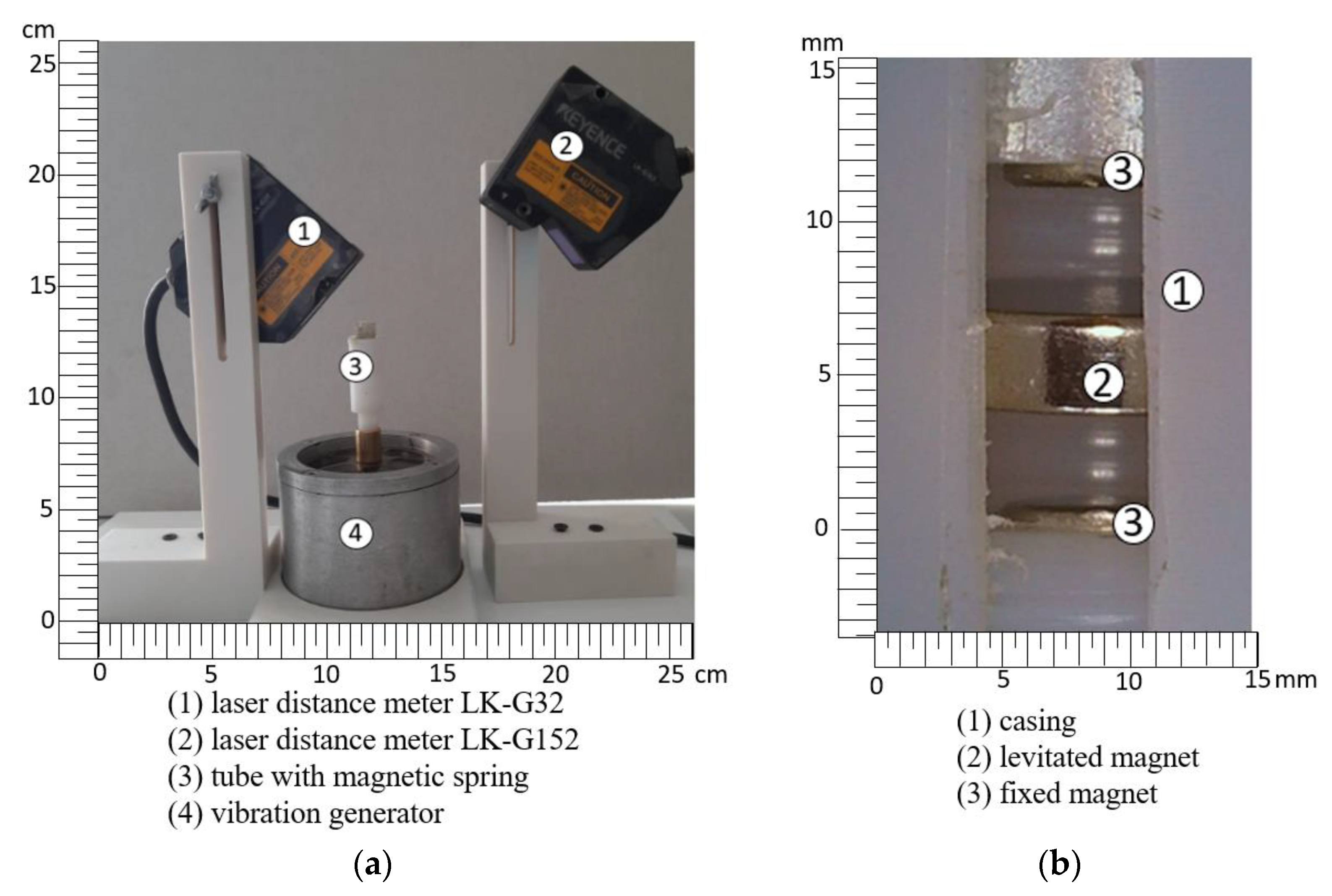
In the previous paper [17], the authors show a 1-DoF model of the magnetic spring in an electromagnetic energy harvester. The electromagnetic energy harvester consists of the mechanical system—the magnetic spring and the electromagnetic system—coils, and magnets. The energy harvesting system structure, which consists of axially magnetized cylindrical permanent magnets in a magnetic spring and a coil located around the magnetic spring, is shown in Figure 2a. In the magnetic spring, the fixed magnets are placed at the top and bottom of the magnetic spring and a levitated magnet is located between them. The levitation of the magnet is ensured by the repulsion force of the fixed magnets and the levitated magnet. The low height of the levitated magnet enables its rotation and causes its instability for higher air gaps between the magnets in the magnetic spring. The casing that contains the magnetic spring has a gap which reduces pressure inside the magnetic spring and also allows the levitated magnet to move with lower air resistance. 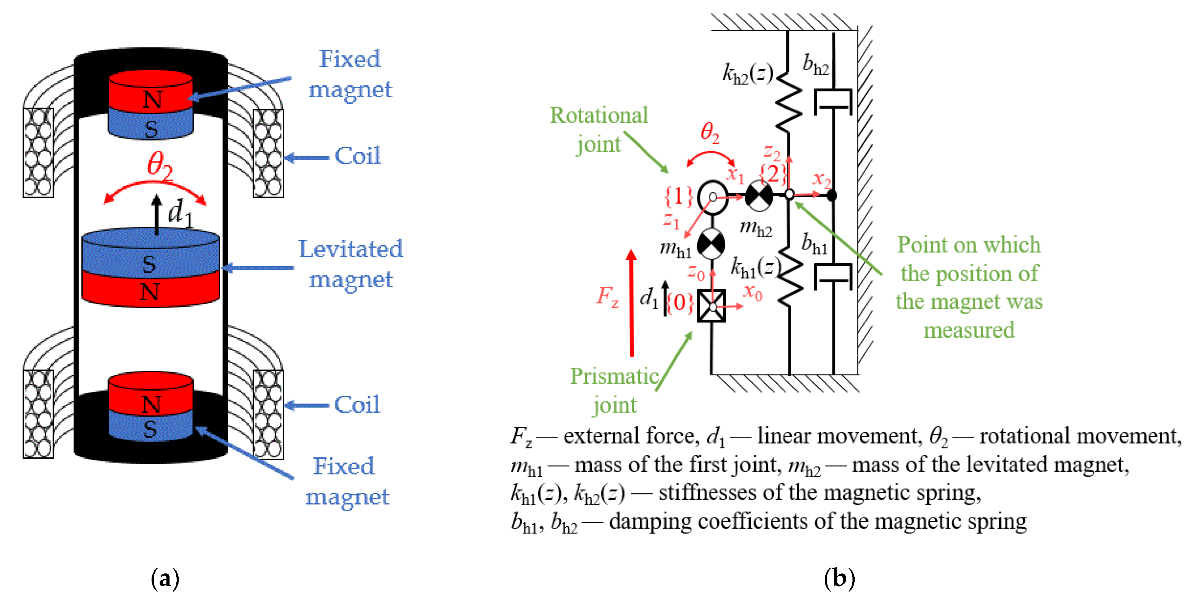In Figure 2a, the levitated magnet moves linearly along the symmetry axis z and rotates around the axis perpendicular to its symmetry axis, as described by the θ angle. The voltage is induced in the coils due to the relative movement of the magnet and coils. For its calculation, Lorentz’s law has been used.

The repulsive forces of fixed and levitated magnets are considered as spring and damping forces; therefore, the magnetic spring with one moveable permanent magnet which levitates between two fixed magnets can be modeled as the mass between two springs and dampers. The novel approach of the magnetic spring modeling is based on the 2-DoF kinematic chain presented in Figure 2b. The linear movement of the levitated magnet along the magnetization axis is illustrated by the prismatic joint and rotational movement around the radial axis by the rotational joint.

In Figure 2b, the mass m_h1 is the symbolic representation of the mass center for the first joint and the mass of the levitated magnet is m_h2. In this case, the value of mass m_h1 is equal to 0. The stiffnesses of the springs k_h1(z) and k_h2(z) have the same value equal to ½ of the magnetic spring’s stiffness. The stiffnesses of the springs k_h1(z) and k_h2(z) depend on the position of the magnet. The damping coefficients b_h1 and b_h2 of the magnetic spring are equal and were calculated using optimization in Matlab [17]. The force F_z is the external force caused by the vibration generator movement. The magnetic spring is acting as an inertial generator; therefore, the force F_z is considered an inertial force (1):

$$F_z=m_h{a}_v$$

(1)

where m_h is the the proof mass and the levitated magnet mass, and a_v is the acceleration of the vibration generator [5].

The equations describing the levitated magnet movement are derived using the Denavit–Hartenberg notation [15].

Table 1. Kinematic parameters of the 2-DoF kinematic chain representing the magnetic spring.

i	ai	αi	di	θi
1	0	$\frac{\mathsf{\pi }}{2}$	d1 *	0
2	a2	$-\frac{\mathsf{\pi }}{2}$	0	θ2 *

presents the kinematic parameters of the kinematic chain shown in Figure 2b), where i is the ordinal number of the link relative to the kinematic chain, a_i is the distance between axes z_i and z_i-1, α_i is the angle between axes z_i and z_i-1, d_i is the distance between axes x_i and x_i-1, θ_i is the angle between axes x_i and x_i-1, d₁ * is the displacement of the prismatic joint, and θ₂ * is the displacement of the rotational joint. The * sign means that the parameter changes with the time.

The kinematic parameters for the gravity centers are presented in

Table 2. Kinematic parameters of the gravity centers of the 2-DoF kinematic chain representing the magnetic spring.

i	ai	αi	di	θi
1	0	0	dc1 *	0
2	ac2	0	0	θc2 *

.

The homogenous transformation is obtained by rotation around the x and z axes and translation along the x and z axes. The homogenous transformations A_i for each joint formulated based on Table 1 and Table 2 can be presented in (2):

$${\mathit{A}}_{\mathrm{i}}=\left[\begin{array}{cc}\begin{array}{cc}{\mathrm{c}\theta }_i& {-\mathrm{s}\theta }_i{\mathrm{c}\alpha }_i\\ {\mathrm{s}\theta }_i& {\mathrm{c}\theta }_i{\mathrm{c}\alpha }_i\end{array}& \begin{array}{cc}{\mathrm{s}\theta }_i{\mathrm{s}\alpha }_i& a_i{\mathrm{c}\theta }_i\\ {-\mathrm{c}\theta }_i{\mathrm{s}\alpha }_i& a_i{\mathrm{s}\theta }_i\end{array}\\ \begin{array}{cc}0& {\mathrm{s}\alpha }_i\\ 0& 0\end{array}& \begin{array}{cc}{\mathrm{c}\alpha }_i& d_i\\ 0& 1\end{array}\end{array}\right]$$

(2)

where cθ_i = cosθ_i, sθ_i = sinθ_i, cα_i = cosα_i, and sα_i = sinα_i.

The homogenous transformation for the whole kinematic chain T₂ is given by (3):

$${\mathit{T}}_2{=\mathit{A}}_1{\mathit{A}}_2=\left[\begin{array}{cccc}{\mathrm{c}\theta }_2& 0& {-\mathrm{s}\theta }_2& a_2{\mathrm{c}\theta }_2\\ 0& 1& 0& 0\\ {\mathrm{s}\theta }_2& 0& {\mathrm{c}\theta }_2& d_1{+a}_2{\mathrm{s}\theta }_2\\ 0& 0& 0& 1\end{array}\right]$$

(3)

where d₁ is the position of the levitated magnet in the direction of the magnetization, θ₂ is the rotation of the magnet around the radial axis of the magnetization, and a₂ is the radius of the levitated magnet.

The homogenous transformation for the last gravity center T_c2 is shown in (4):

$${\mathit{T}}_{\mathrm{c}2}{=\mathit{A}}_1{\mathit{A}}_{\mathrm{c}2}=\left[\begin{array}{cccc}{\mathrm{c}\theta }_2& {-\mathrm{s}\theta }_2& 0& a_{\mathrm{c}2}{\mathrm{c}\theta }_2\\ 0& 0& -1& 0\\ {\mathrm{s}\theta }_2& {\mathrm{c}\theta }_2& 0& d_1{+a}_{\mathrm{c}2}{\mathrm{s}\theta }_2\\ 0& 0& 0& 1\end{array}\right]$$

(4)

where a_c2 is the distance between the geometry center of the levitated magnet and the gravity center of the levitated magnet.

To obtain equations of the levitated magnet movement, the Euler–Lagrange equation can be used:

$$\mathit{D}[\begin{array}{c}{\ddot{d}}_1\\ \ddot{{\theta }_2}\end{array}]+\mathit{C}[\begin{array}{c}{\dot{d}}_1\\ \dot{{\theta }_2}\end{array}{]+[F}_{\mathrm{pi}}{]=[F}_{\mathrm{i}}{-F}_{\mathrm{bi}}]$$

(5)

where D is the inertia matrix, C is the Christoffel matrix, F_pi is the potential force or torque acting on the i joint, F_i is the external force or torque acting on the i joint, and F_bi is the damping forces or torques acting on the i joint.

The inertia matrix D is obtained as a part of a kinetic energy E_k:

$$E_{\mathrm{k}}=\frac{1}{2}{\dot{\mathit{q}}}^{\mathrm{T}}{\displaystyle \sum }_{i=1}^n(m_i{\mathit{J}}_{vci}^{\mathrm{T}}(q){\mathit{J}}_{vci}(q)+{\mathit{J}}_{\omega ci}^{\mathrm{T}}(q){\mathit{R}}_i(q){\mathit{I}}_i{\mathit{R}}_i^{\mathrm{T}}(q){\mathit{J}}_{\omega ci}(q))\dot{\mathit{q}}=\frac{1}{2}{\dot{\mathit{q}}}^{\mathrm{T}}\mathit{D}(q)\dot{\mathit{q}}$$

(6)

where J_vi is the Jacobian matrix of the linear speed of the i joint, J_wi is the Jacobian matrix of the rotational speed of the i joint, m_i is the mass of the i link, I_i is the moment of inertia of the i link, and q is the joint displacement [15].

The Jacobian matrix of the linear and rotational speed can be obtained by the z-axis and the coordinate of the joint center [15]. The Jacobian matrix for the prismatic joint gravity center J_c1 can be obtained by Equation (7) and the rotational joint gravity center J_c2 by Equation (8):

$${\mathit{J}}_{\mathrm{c}1}=\left[\begin{array}{cc}{\mathit{J}}_{\mathrm{vc}1}& 0\\ {\mathit{J}}_{\mathsf{\omega }\mathrm{c}1}& 0\end{array}\right]=\left[\begin{array}{cc}{\mathit{z}}_0& 0\\ 0& 0\end{array}\right]=\left[\begin{array}{cc}0& 0\\ 0& 0\\ 1& 0\\ 0& 0\\ 0& 0\\ 0& 0\end{array}\right]$$

(7)

where the z₀ is referred to the base coordinate system {0}—[0,0,1] (Figure 2).

$${\mathit{J}}_{\mathrm{c}2}=\left[\begin{array}{cc}{\mathit{J}}_{\mathrm{v}1}& {\mathit{J}}_{\mathrm{vc}2}\\ {\mathit{J}}_{\mathsf{\omega }1}& {\mathit{J}}_{\mathsf{\omega }\mathrm{c}2}\end{array}\right]=\left[\begin{array}{cc}{\mathit{z}}_0& {\mathit{z}}_1\times \left({\mathit{o}}_{\mathrm{c}2}{-\mathit{o}}_1\right)\\ 0& {\mathit{z}}_1\end{array}\right]=\left[\begin{array}{cc}0& {-a}_{\mathrm{c}2}{\mathrm{s}\theta }_2\\ 0& 0\\ 1& a_{\mathrm{c}2}{\mathrm{c}\theta }_2\\ 0& 0\\ 0& -1\\ 0& 0\end{array}\right]$$

(8)

where o_c2 is the center of the second gravity center, o₁ is the center of the first gravity center, and z₁ is referred to in Figure 2.

The external force F_i expressed in the coordinate system of the the i joint is calculated by Equation (9):

$$\left[F_i\right]={\mathit{J}}_{c2}{}^{\mathit{T}}\left[\begin{array}{c}0\\ 0\\ F_z\\ 0\\ 0\\ 0\end{array}\right]=\left[\begin{array}{c}{F}_z\\ F_z{a}_{c2}c{\theta }_2\end{array}\right]$$

(9)

The inertia matrix is:

$$\mathit{D}=\left[\begin{array}{c}\begin{array}{c}\begin{array}{cc}{m}_1{+m}_2& a_{\mathrm{c}2}{m}_2{\mathrm{c}\theta }_2\\ a_{\mathrm{c}2}{m}_2{\mathrm{c}\theta }_2& m_2{a}_{\mathrm{c}2}{}^2{+I}_2\end{array}\end{array}\end{array}\right]$$

(10)

where m₁ is the mass of the first joint and is equal to 0, m₂ is the mass of the levitated magnet, and I₂ is the moment of inertia of the levitated magnet calculated along the radius.

The Christoffel matrix is calculated by the inertia matrix D [15], as shown in Equation (11):

$$\mathit{C}=\left[\begin{array}{cc}\begin{array}{c}0\\ 0\end{array}& \begin{array}{c}{-{\dot{\theta }}_{2}a}_{\mathrm{c}2}{m}_2{\mathrm{s}\theta }_2\\ 0\end{array}\end{array}\right]$$

(11)

where ${\dot{\theta }}_2$ is the rotational velocity of the levitated magnet.

Finally, the movement of the levitated magnet can be presented by Equation (12):

$$\begin{gathered} \left[\begin{array}{c}{d}_1\\ {\theta }_2\end{array}\right]=\frac{F_z\left(I_2+{a_{c2}}^2{m}_2-{a_{c2}}^2{m}_2{c}^2{\theta }_2\right)-F_{\mathrm{p}1}\left(I_2+{a_{c2}}^2{m}_2\right)-F_{\mathrm{b}1}\left(I_2+{a_{c2}}^2{m}_2\right)+{\tau }_{\mathrm{p}2}{a}_{\mathrm{c}2}{m}_2{\mathrm{c}\theta }_2+{\tau }_{\mathrm{b}2}{a}_{\mathrm{c}2}{m}_2{\mathrm{c}\theta }_2+{a_{c2}}^3{{\dot{\theta }}_2}^2{m_2}^{2}s{\theta }_2+I_2{a}_{c2}{{\dot{\theta }}_2}^2{m}_{2}s{\theta }_2}{-{a_{c2}}^2{m_2}^2{c}^2{\theta }_2+{a_{c2}}^2{m_2}^2+I_2{m}_2} \\ \frac{-{a_{c2}}^2{{\dot{\theta }}_2}^2{m_2}^2\mathrm{c}{\theta }_{2}s{\theta }_2-{\tau }_{\mathrm{p}2}{m}_2-{\tau }_{\mathrm{b}2}{m}_2+F_{\mathrm{p}1}{a}_{\mathrm{c}2}{m}_2{\mathrm{c}\theta }_2+F_{\mathrm{b}1}{a}_{\mathrm{c}2}{m}_2{\mathrm{c}\theta }_2}{-{a_{c2}}^2{m_2}^2{c}^2{\theta }_2+{a_{c2}}^2{m_2}^2+I_2{m}_2} \end{gathered}$$

(12)

where F_p1 is the potential force acting on the first joint and the spring force of the magnetic force presented in Equation (15), F_b1 is the damping force acting on the first joint presented in Equation (13), τ_p2 is the potential and damping torque acting on the second joint presented in Equation (16), and τ_b2 is the damping torque acting on the second joint presented in Equation (14). The spring constant force and gravitational force are in equilibrium.

$$F_{\mathrm{b}1}{=b}_1{\dot{d}}_1$$

(13)

where b₁ is the linear damping of the spring and ${\dot{d}}_1$ is the linear velocity of the levitated magnet.

$${\tau }_{\mathrm{b}2}{=b}_2{\dot{\theta }}_2$$

(14)

where b₂ is the rotational damping of the spring, and ${\dot{\theta }}_2$ is the rotational velocity of the levitated magnet.

The resonance frequency and movement of the levitated magnet in a magnetic spring depend on the spring force and the torque value. The spring force and torque change with the displacement. Thus, the relationship between the force and torque to linear and rotational displacement of the levitated magnet has been determined using the simulation modeling conducted in ANSYS Maxwell 3D.

In the magnetic spring, the repulsive force of the two magnets is considered a nonlinear restoring force depending on the magnetic field intensity, distance of the magnet, and potential energy [10]. Therefore, the passive nonlinear spring force acts on the levitated magnet [7,10,11]. In this simulation model, the force in the magnetic spring is considered a combination of two parallel spring forces of equal intensity.

The magnetic property of the magnets used in the simulation model of the magnetic spring is a relative magnetic permeability of 1.0535 and a magnetic coercivity of 800 kA/m. The magnetic coercivity used in the simulation differs from that given by the producer (937.4 kA/m) [18]. Magnets in the magnetic spring have different manufactured properties and are probably demagnetized during vibration tests. The coercivity in the simulation was obtained based on the magnetic repulsive forces measured between the levitated magnet and the external magnet.

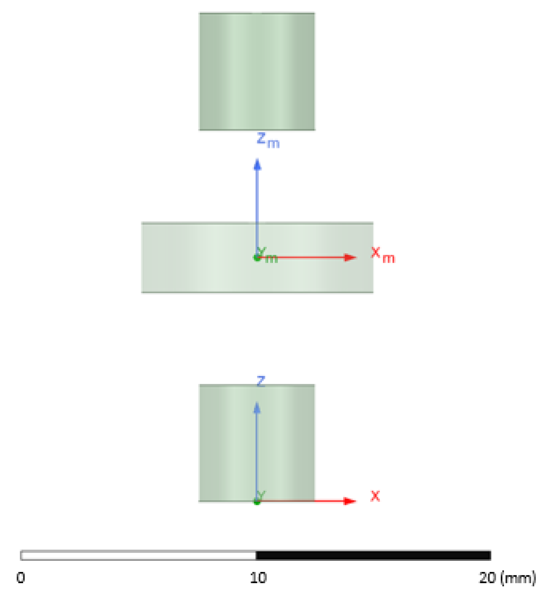
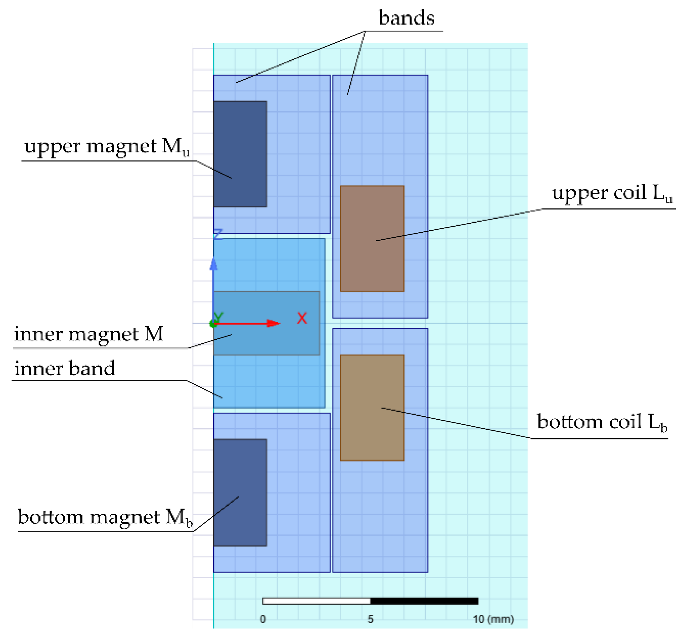
In the simulation model, the levitated magnet moves linearly and rotates. The force was calculated along the z-axis and torque was considered around the x_m-axis (Figure 3). The exterior boundaries were set to Neumann boundaries and the interior boundaries between magnets were set to natural boundaries.

The levitated magnet changes its position linearly along the z-axis direction in the range of −3.2 mm to 3.2 mm and also rotationally around the x_m-axis in the range of 0° to 10°. The force approximation and torque equation by Matlab are presented, respectively, in Equations (15) and (16):

$$F_{\mathrm{p}1}{(z,\theta )=p}_{\mathrm{f}70}{d}_1{}^7{+p}_{\mathrm{f}61}{d}_1{}^6{\theta }_2{+p}_{\mathrm{f}60}{d}_1{}^6{+p}_{\mathrm{f}52}{d}_1{}^5{\theta }_2{}^2{+p}_{\mathrm{f}51}{d}_1{}^5{\theta }_2{+p}_{\mathrm{f}50}{d}_1{}^5{+\dots +p}_{\mathrm{f}12}{d}_1{\theta }_2{}^2{+p}_{\mathrm{f}11}{d}_1{\theta }_2{+p}_{\mathrm{f}10}{d}_1{+p}_{\mathrm{f}00}$$

(15)

$${\tau }_{\mathrm{p}2}{(z,\theta )=p}_{\mathrm{t}60}{d}_1{}^6{+p}_{\mathrm{t}51}{d}_1{}^5{\theta }_2{+p}_{\mathrm{t}50}{d}_1{}^5{+p}_{\mathrm{t}42}{d}_1{}^4{\theta }_2{}^2{+p}_{\mathrm{t}41}{d}_1{}^4{\theta }_2{+p}_{\mathrm{t}40}{d}_1{}^4{+\dots +p}_{\mathrm{t}12}{d}_1{\theta }_2{}^2{+p}_{\mathrm{t}11}{d}_1{\theta }_2{+p}_{\mathrm{t}10}{d}_1{+p}_{\mathrm{t}00}$$

(16)

where d₁ is the position of the levitated magnet, θ₂ is the angle of the rotational variation of the levitated magnet, p_f00, …, p_f70 are coefficients of the force approximation equation, and p_t00, …, p_t60 are coefficients of the torque approximation equation. These coefficients are shown, respectively, in

Table 3. Coefficients of approximating polynomials of the magnetic force.

Coefficients	F1	Coefficients	F1	Coefficients	F1
pf00	−2.722 × 10−4	pf01	−3.933 × 10−5	pf02	1.819 × 10−5
pf10	−0.528	pf11	4.439 × 10−4	pf12	−8.381 × 10−5
pf20	5.516 × 10−4	pf21	−3.026 × 10−4	pf22	2.552 × 10−5
pf30	−8.839 × 10−3	pf31	−2.663 × 10−4	pf32	4.041 × 10−5
pf40	−9.927 × 10−5	pf41	4.18 × 10−5	pf42	−3.334 × 10−6
pf50	3.023 × 10−4	pf51	2.141 × 10−5	pf52	−1.275 × 10−6
pf60	−4.222 × 10−6	pf61	−5.648 × 10−7
pf70	8.719 × 10−6

and

Table 4. Coefficients of approximating polynomials of the magnetic torque.

Coefficients	τ2	Coefficients	τ2	Coefficients	τ2
pt00	−1.453 × 10−6	pt01	−1.218 × 10−4	pt02	−8.364 × 10−8
pt10	3.055 × 10−6	pt11	−1.97 × 10−6	pt12	2.304 × 10−7
pt20	9.485 × 10−6	pt21	−8.295 × 10−6	pt22	−1.351 × 10−7
pt30	−4.63 × 10−7	pt31	9.043 × 10−8	pt32	−2.009 × 10−8
pt40	−2.757 × 10−6	pt41	4.552 × 10−7	pt42	1.484 × 10−8
pt50	3.719 × 10−8	pt51	4.386 × 10−9
pt60	1.853 × 10−7

.

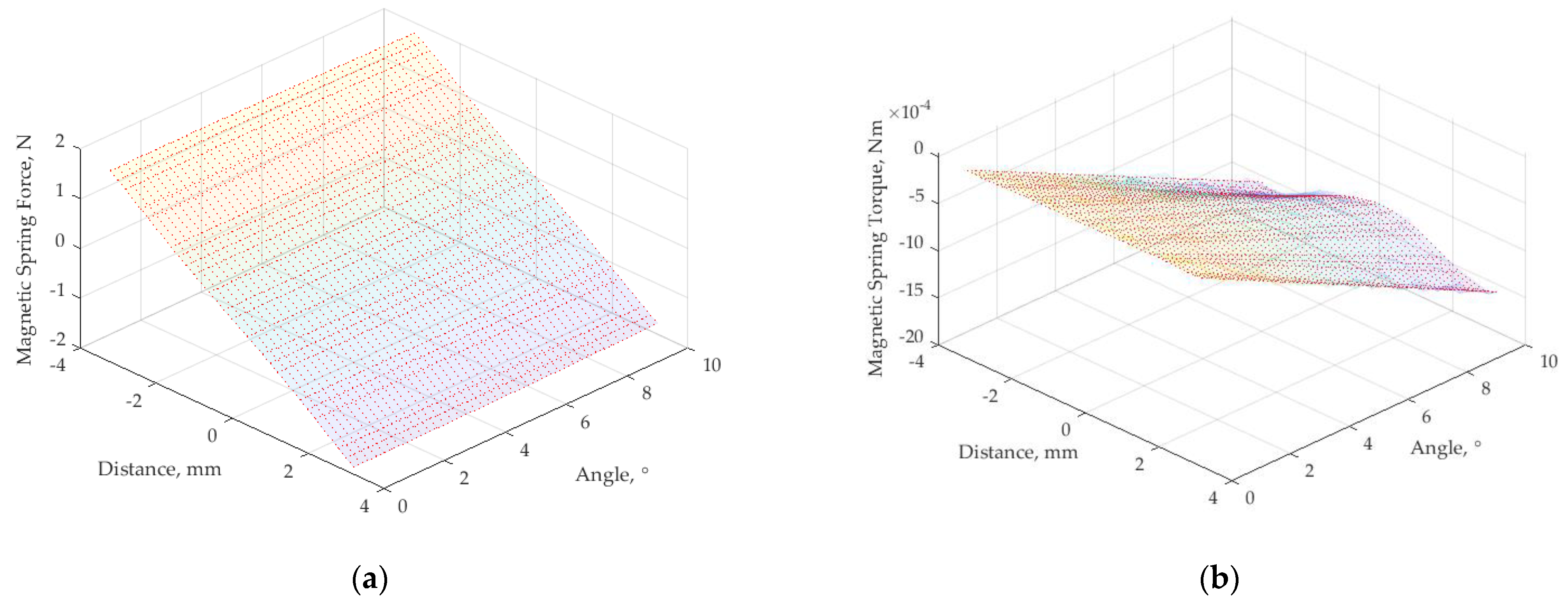
The force and torque, as a function of the linear and rotational position of the levitated magnet are presented, respectively, in Figure 4a,b.

In Figure 4a, the force changes as a function of the rotational angle of the levitated magnet, especially when the levitated magnet is near the fixed magnet. The force values vary from −1.5 N to 1.5 N. In Figure 4b, the lower torque values in the range between 0 Nm and −1.5 × 10⁻³ Nm are due to the low values of the magnetic field intensity during the rotational movement of the levitated magnet. The highest value of the torque is reached for the highest rotational angle of the levitated magnet. The torque value is the lowest when the levitated magnet is in the middle position between the fixed magnets. Therefore, the entire spring is affected more by the applied force than the torque.

The displacement of the levitated magnet d_m for a 2-DoF magnetic spring in the z₀-axis (Figure 2) is calculated as:

d_m= d_c1+a₂sin(θ₂)

(17)

where d_c1 is the linear displacement of the levitated magnet, a₂ is the radius of the levitated magnet, and θ₂ is the angular position of the levitated magnet.

In this paper, only the theoretical analysis of generated electrical power of an electromagnetic generator was conducted. Two coils connected in series, wounded around a magnetic spring using copper wire at a diameter of 0.18 mm with 400 turns, with 5 mm of height, 12 mm of internal diameter, and 18 mm of external diameter were considered. In the coil, the voltage is induced according to Faraday’s law. In this case, the transducer force F_T (18), derived from the induced voltage, is included in the external force Equation (1):

$$F_{\mathrm{T}}=\frac{e^2{R}_L}{{\left(2R_c+R_L\right)}^2\dot{d_m}}$$

(18)

where R_L is the the load resistance, R_C is the resistance of the one coil, and e is the induced voltage.

The voltage induced in the coils takes the form:

$$e=-\frac{\partial \varphi }{\partial d_{\mathrm{m}}}\frac{\partial d_{\mathrm{m}}}{\partial t}$$

(19)

where d_m is the displacement of the magnet, and ϕ is the magnetic flux.

This force causes additional damping in the movement of the levitated magnet. The external force F_z (1) is given by:

$$F_z=m_h{a}_v-F_{\mathrm{T}}$$

(20)

The magnetic flux in coils was calculated in ANSYS Maxwell. The magnetic flux approximation equation by Matlab is defined as:

$$\varphi {\left(d_{\mathrm{m}}\right)=p}_3{d_{\mathrm{m}}}^3{+p}_2{d_{\mathrm{m}}}^2{+p}_1{d}_{\mathrm{m}}$$

(21)

where d_m is the relative displacement of the levitated magnet in coil, and p₁, p₂, and p₃ are coefficients of the magnetic flux approximation equation. These coefficients are shown in

Table 5. Coefficients of approximating polynomials of the magnetic flux for first coil ϕ₁ and second coil ϕ₂.

Coefficients	ϕ1	Coefficients	ϕ2
p1	−2.267 × 10−3	p1	2.265 × 10−3
p2	−1.418 × 10−1	p2	−1.161 × 10−1
p3	−8.599	p3	−7.507

for each coil, respectively.

The electrical power obtained by an electromagnetic generator can be calculated by:

$$P=\frac{e^2{R}_L}{{\left(2R_c+R_L\right)}^2}$$

(22)

The maximum power is generated when the load resistance is equal to the resistance of the coil.

2.3. The Neural Network Model of the Vibration Generator

The vibration generator movements affect the magnetic spring displacement. In order to control the vibrations, the mathematical model presented in the literature of the vibration generator needs to be improved. The vibration generator displacement amplitude and frequency characteristic are nonlinear and complex. Therefore, in this research, the vibration generator is modeled using an artificial neural network (ANN) in order to establish an accurate relation between the amplitude and frequency of current and the amplitude of vibration generator displacement obtained by measurements in the laboratory. The ANN can work continuously and more efficiently than the analytical model and provides a high accuracy after extensive parameter optimization, contrary to the SVM model. Basically, SVM utilizes nonlinear mapping to make the data linear and separable; hence, the kernel function is the key. However, the ANN employs multi-layer connection and various activation functions to deal with nonlinear problems, as in this case.

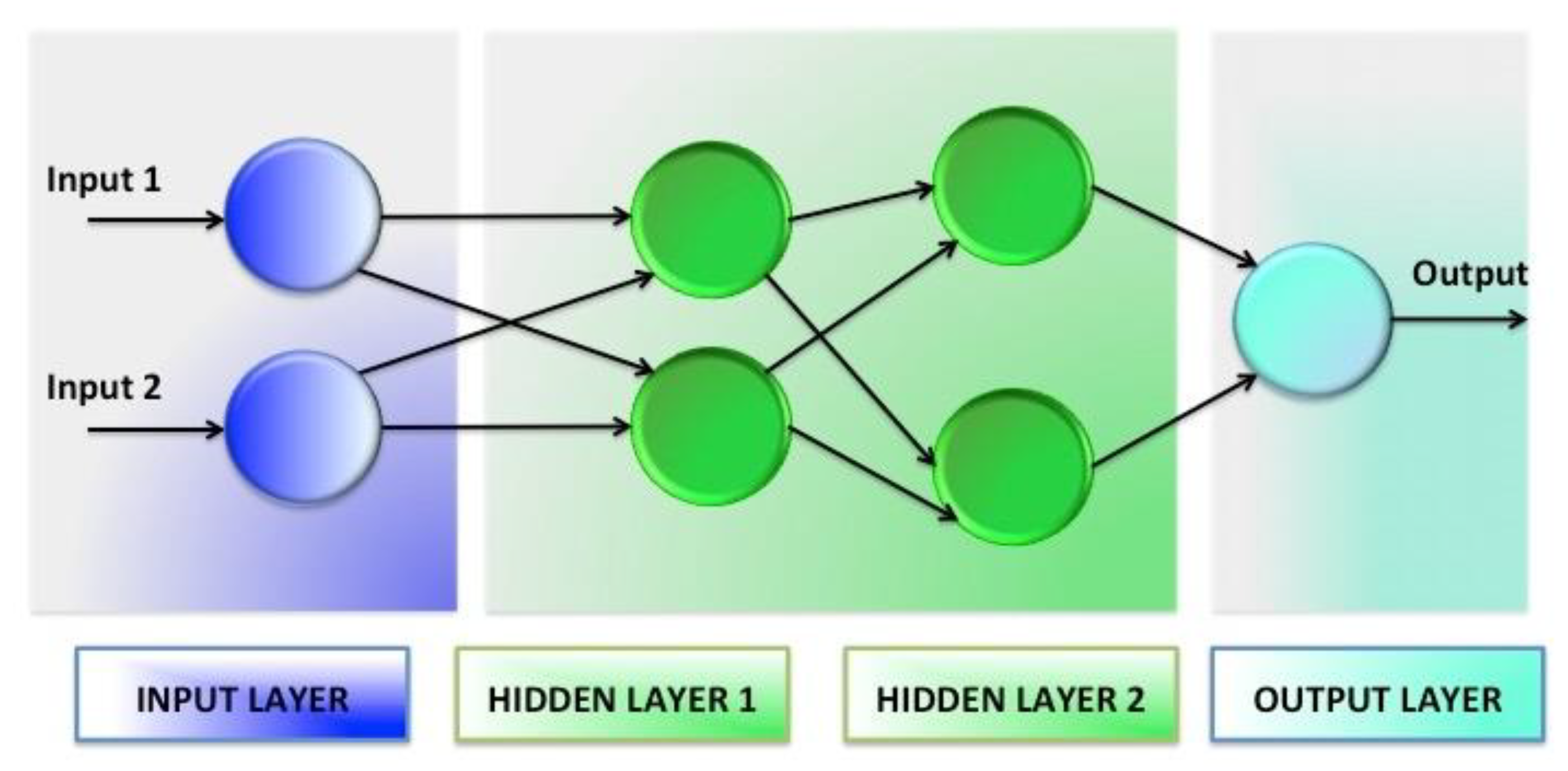
The ANN is able to perform computational tasks involving multiple entities called neurons (neurons), organized in a network divided into levels (layers), which calculate the value of parameters (weight) useful to minimize a cost function. ANNs are composed of an input layer, one or more hidden layers, and an output layer. Each node, or artificial neuron, has an associated weight and threshold. Each layer, except the last one, is fully connected with neurons to the subsequent layer. A bias neuron represents a biasing feature and produces 1 output in every situation. Input–output transfer functions of neural networks can be easily obtained by a supervised learning process based on empirical data. The network is trained by a suitable algorithm, usually a backpropagation learning algorithm. The latter is used to change the weights w_i and parameters (thresholds) within the same network to minimize the sum of the squared error functions. The weight of an input is the number which, when multiplied by the input x_i, gives the weighted input. The function g is the unit’s activation function:

$$y\left(x\right)=g\left({\displaystyle \sum }_{i=1}^d{\mathit{w}}_i{\mathit{x}}_i{+\mathit{w}}_0\right)$$

(23)

where

$${\mathit{w}}_1=iw[1,1], {\mathit{w}}_2=iw[1,2],{\mathit{b}}_1=b\left[1\right],{\mathit{b}}_2=b\left[2\right]$$

(24)

Each input weight, layer weight, and bias vector has as many rows as the size of the i layer, after the training network bias and weights change. In our case, iw [1,1] is the weight to layer 1 from input 1, iw [1,2] is the weight to layer, b [1] is the bias to layer 1, and b [2] is the bias to layer 2. In a multi-layer feed-forward neural network, artificial neurons are arranged in layers, and all the neurons in each layer are connected to all neurons in the next layer. Each connection between these artificial neurons is assigned a weight value that represents the weight of the connection.

Given the frequency and amplitude current input values of the vibration generator, the neural network feedforward is used to compute the amplitude of the movement of the vibration generator at the output of the multi-layer perceptron (MLP) neural network. In the feedforward process, external input values are first multiplied by their weights and summed. The output y = f(x) is a weighted sum function, called the activation function. The relation between the input variable X and the output variable Y is achieved by adjusting the parameters and weights to reduce errors. The process of finding a set of weights so that the network produces the desired output for a given input is called training. Neural networks learn the relations between different input and output patterns.

The feedforward backpropagation neural network was used to determine a nonlinear mapping from the input vector of the current, specifically frequency and amplitude, and the amplitude of vibration. The input x is defined as a vector of frequency and amplitude of the current whose waveform was obtained by signal generator AGILENT 33210a amplified by amplifier IRS2092. The amplitude of the current was calculated using fast Fourier transform (FFT). The output y(x) is expressed by the amplitude of the vibration generator obtained by the FFT applied to the signal of laser distance meters LK-G32 (25). The training dataset for the network has 140 samples and the validation dataset has 70 samples. The feedforward backpropagation neural network is composed of the input layer with two neurons arranged in the first hidden layer and other two neurons arranged in the second hidden layer using a Log-sigmoid transfer function (logsig), and an output layer with hyperbolic tangent sigmoid transfer function (tangsig), as shown in Figure 5.

The hyperbolic tangent function has the properties to be differentiable and the output has a range of values of [−1, 1] (different from that [0, 1] of the logistic function), which leads each output of the level to be more or less normalized (i.e., centered around the value 0) at the beginning of training. This often helps speed convergence. The input–output mathematical relation obtained by the ANN is described as follows:

$$y\left(\mathit{x}\right)=\mathrm{tansig}\left({\mathit{W}}_o\mathrm{logsig}\left({\mathit{W}}_h\mathrm{logsig}\left({\mathit{W}}_i{\mathit{x}+\mathit{b}}_i\right){+\mathit{b}}_h\right){+\mathit{b}}_o\right)$$

(25)

where W_i is an array containing weights to layer 1 from input 1, W_h is an array containing weights to the hidden layer, W_o is an array containing weights to the output layer, b_i is an array containing bias values to layer 1, b_h is an array containing bias values to hidden layer 2, and b_o is an array containing bias values to the output layer. The weights and biases are shown in

Table 6. Values of weights and biases for the neural network model of the vibration generator.

Name	Values Obtained by the ANN Model	Details
Wi	[2.7365 0.028886; 17.1944 −0.055445]	Weights to layer 1 from input 1
Wh	[−0.53955 2.742; −9.1492 9.123]	Weights to the hidden layer
Wo	[−7.2542 9.7889]	Weights to the output layer
bi	[2.6625; 13.5824]	Bias to layer 1
bh	[−0.11812; −3.5193]	Bias to layer 2
bo	[4.0911]	Bias to the output layer

.

The mechanism to update the weight and bias values corresponding to Levenberg–Marquardt optimization was conducted using the network training function (trainbr). The process called Bayesian regularization using trainbr has combined the minimization of the squared error and weights of the network in order to generalize the ANN. The gradient descent with momentum weight and bias learning function (learngdm) is selected for the calculation. The learning curve has exhibited the good performance of the ANN and after 293 epochs obtained an MSE of 0.036 and an excellent generalization due to the fact that the test curve is always under the training curve, as shown in Figure 6.

2.4. The Simulink Model of Magnetic Spring Based on the Input Signal of the Vibration Generator Obtained by the Neural Network

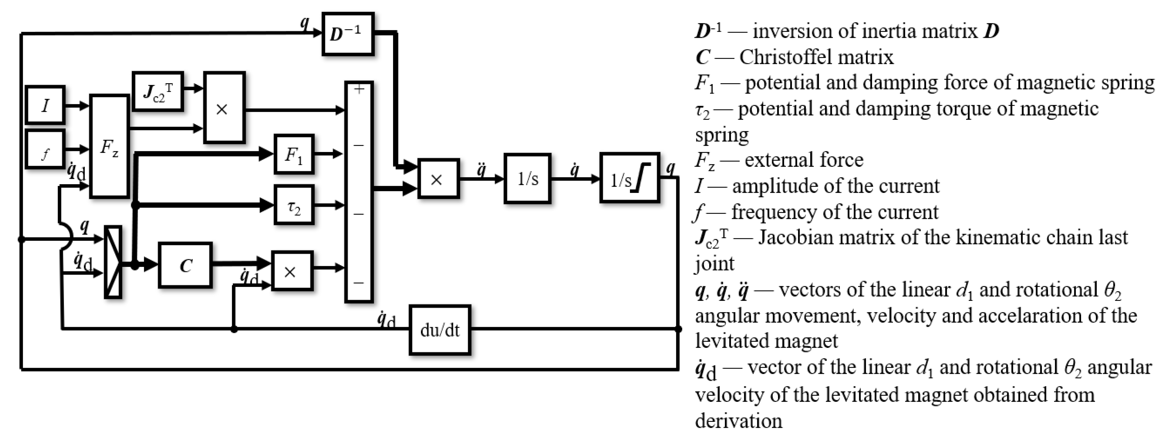
The magnetic spring and the vibration generator were designed and simulated using a block diagram by Simulink/Matlab to define the mathematical relation between the input (current of vibration generator) and output (displacement of magnetic spring) signal, including the results obtained by the 2-DoF kinematic chain model (12), the ANN (25), and simulation modeling in ANSYS (15) and (16). The input signal of the model is represented by the amplitude and frequency values of the current that supply the vibration generator. The force generated by the vibration generator is the input of the magnetic spring model. The output of the simulated model is represented by the linear and rotational displacement of the magnetic spring. The magnetic spring model is controlled by the magnetic spring force and torque that depend on its displacement. The used model algorithm represents the physical system in multidomain blocks (Figure 7).

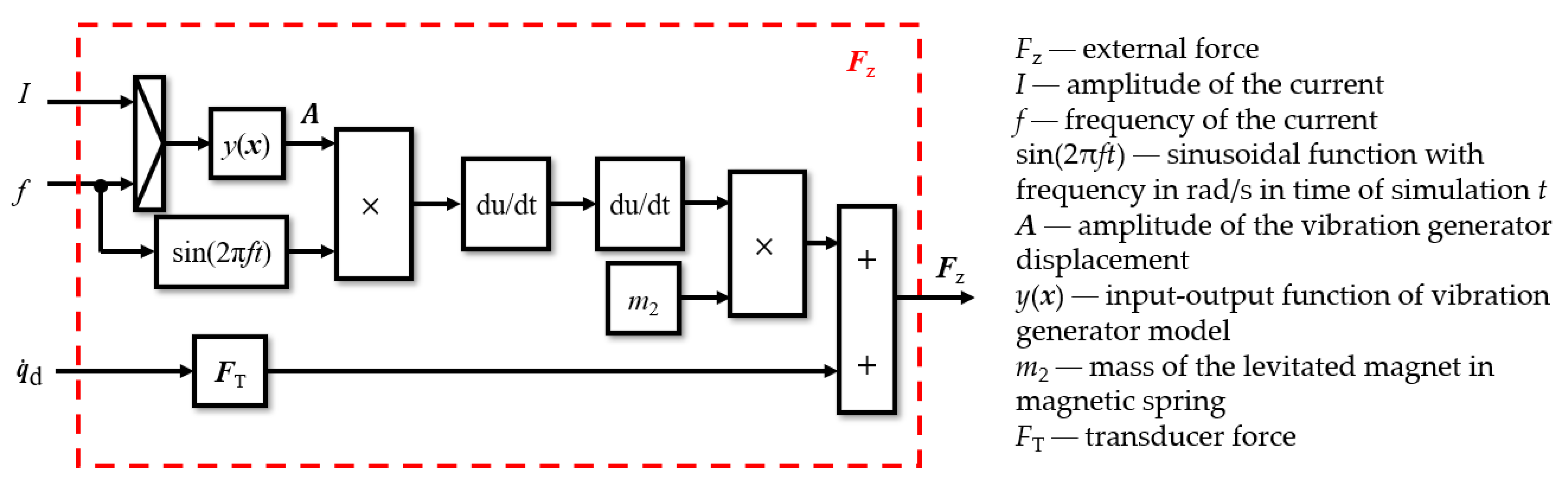
The displacement of the vibration generator is obtained by the input–output equation based on the ANN (Figure 8).

In the simulation model (Figure 7), the inputs I and f are, respectively, the current amplitude and frequency of the vibration generator. The neural network of the vibration generator is identified by the block F_z shown in Figure 8. In Figure 7, the transposition of the Jacobian of the second joint mass center J_c2^T is obtained by Equation (8). The potential force presented in Equation (15) and damping force for the first joint presented in Equation (13) are contained in block F₁. The potential torque presented in Equation (16) and damping torque for the second joint presented in Equation (14) are contained in block τ₂. The inversion of the inertia matrix D presented in Equation (10) and Christoffel matrix C presented in Equation (11) are contained, respectively, in blocks D⁻¹ and C. The result of the model is vector q of the linear and rotational movement of the levitated magnet. In integration blocks, 1/s acceleration and velocity of the levitated magnet are integrated. The movement of the magnet is limited by the magnetic spring design. The derivation block du/dt is a derivative of the position of the levitated magnet velocity.

In Figure 8, block y(x) contains the input–output function for the vibration generator model by the ANN presented in Equation (25). The block sin(2πft) contains a sinusoidal function with the input frequency f and simulation time t. The m₂ contains the mass of the levitated magnet.

The mass of the levitated magnet m₂ is 1.77 × 10⁻³ kg and the inertia moment I₂ of the levitated magnet around the axis perpendicular to linear movement is calculated from the magnet’s height and radius and equals 1.24 × 10⁻⁸ kgm². The distance a₂ between the geometry center of the levitated magnet and the point on which the movement was measured is equal to the radius of the levitated magnet 5 × 10⁻³ m. The distance a_c2 between the geometry center of the levitated magnet and the gravity center of the levitated magnet is assumed to be equal to 5 × 10⁻⁴ m. The linear damping coefficients b_h1 and b_h2 were calculated in the optimization process and each equals 0.045 Ns/m. The linear damping coefficient of the whole magnetic spring b₁ is the sum of the linear damping coefficients b_h1 and b_h2 and it is equal to 0.09 Ns/m. The rotational damping coefficient b₂ of the whole magnetic spring is equal to 2 × 10⁻⁷ Nms/rad.

In order to take into account the electrical power induced by the inertial generator that contains the magnetic spring, the transducer force is included in the external force block diagram. For the simulation of the magnetic spring without a coil transducer force, F_T is equal to 0. For the simulation with the coil transducer force, F_T is calculated based on Equation (18). Transducer force depends on the velocity of the magnet in the coil. The voltage is calculated by Equation (19) and the magnetic flux by Equation (21). The generated power is calculated by Equation (22). The voltage and electrical power depend on the velocity of the levitated magnet. The magnetic flux depends on the position of the levitated magnet. The position and velocity are obtained from the simulation in Simulink. The load resistance equals the resistance of the coil, which is 24 Ω.

2.5. The FEM Transient Model of the Magnetic Spring

To improve the completeness of the research, the energy harvester was analyzed using another FEM model. This model took into account also the current induced by the inner magnet movement and its impact on the characteristic of the whole device. The model, presented in Figure 9, was performed using the Ansys Electronics Desktop program and set up as a 2D transient model, axisymmetric around axis z. All the moving elements of the device have an assigned motion band, which is a type of Ansys object allowing for a movement consideration in the used FEM environment.

In the model, magnets Mu and Mb, and coils Lu and Lb move harmonically along the z-axis, with velocity v set according to the following equation:

$$\mathrm{v}=A\omega cos\left(2\pi ft\right)$$

(26)

where A is the amplitude of the harmonic displacement and f is the frequency of the movement. This harmonic movement generates a variable spring force on the inner magnet M, causing its movement. In this model, only the linear movement of the magnet, along the z-axis was considered. The relative motion of the M magnet and the generating coils causes a time-varying magnetic flux and induces a voltage in the coils. The dimensions and parameters of the model are the same as reported in Section 2.2. The electric power on the purely resistive load R_L was calculated. The possible eddy currents that could be induced in the magnets were omitted in this model.

3. Results and Discussion

3.1. The Displacement Results

The amplitude frequency characteristics results conducted in the laboratory are shown in Figure 10. In order to achieve the amplitude of the vibration generator and levitated magnet movements obtained by laser distance meters, the fast Fourier transformation (FFT) has been performed in Matlab. The red curve in the plot of Figure 5 indicates the amplitude of the vibration generator movement that was measured by the LK-G32 laser distance meter. The blue curve in the plot of Figure 5 indicates the amplitude of the levitated magnet movements in the magnetic spring placed on the vibration generator measured by the LK-G152 laser distance meter.

In Figure 10a,b, the measurements of the vibration generator movements have shown four resonance frequencies of 2 Hz, 30 Hz, 46 Hz, and 68 Hz. For the magnetic spring, the resonance frequency is about 86 Hz. The amplitudes of the levitated magnet movement in the frequency range of 80–120 Hz for input current 0.35 A and 0.75 A are shown in Figure 11a,b, respectively. It can be seen that the magnetic spring has two resonance frequencies. The second resonance frequency of the magnetic spring corresponds with the visible rise of the amplitude of the magnetic spring movement at 106 Hz.

The amplitude frequency characteristics of experimental results for the vibration generator for input current amplitude 0.35 A and 0.75 A are shown in Figure 12a,b, respectively. It can be seen that the higher the input current amplitude, the higher the vibration amplitude of the vibration generator. It can be seen (in Figure 10 and Figure 12) that, for the lower frequencies, the amplitude of displacement of the vibration generator in absence of the magnetic spring is higher than the amplitude of displacement of the vibration generator with the magnetic spring. For the frequencies closer to resonance frequencies of the magnetic spring, the displacement of the loaded vibration generator is higher than for the vibration generator in absence of the magnetic spring. It can be caused by the influence of the levitated magnet movement.

The amplitude as a function of the frequency of the vibration generator and the levitated magnet movements relative to the measurements and simulation model for the input current 0.35 A are shown, respectively, in Figure 13a and Figure 14a. The amplitude as a function of the frequency of the vibration generator and the levitated magnet movements relative to the measurements and simulation model for the input current 0.75 A are shown, respectively, in Figure 13b and Figure 14b.

In Figure 13, two resonance frequencies at 2 Hz and 30 Hz relative to the vibration generator are obtained by the neural network model. In Figure 14, the magnetic spring has two resonance frequencies at 86 Hz and 120 Hz obtained in the simulation model, and two resonance frequencies at 86 Hz and 106 Hz obtained in measurements. Most electromagnetic energy harvesters are designed to work at the resonance frequency for the highest output power. Therefore, more resonance frequencies in the energy harvester are requested for many applications in environmental vibrations caused by wind, tidal waves, vehicles, and human motions.

In order to compare the results for the magnetic spring presented as a 1-DoF kinematic chain [17] and the magnetic spring presented as a 2-DoF kinematic chain, the simulation was repeated for the 1-DoF kinematic chain magnetic spring. The input force was generated by the neural network model of the vibration generator. The amplitude frequency graphs for input current 0.35 A and 0.75 A are shown in Figure 15a,b, respectively.

One resonance frequency is visible on the graphs of a 1-DoF model, as noticed in the previous paper [17]. In the results of the levitated magnet for the 2-DoF model, two resonance frequencies are exhibited, in agreement with the measurement results. The 2-DoF kinematic chain representation is an accurate model for the realized prototype magnetic spring that is useful for two different applications corresponding to two different resonance frequencies. It is more suitable and efficient than the 1-DoF kinematic chain model, from which only one resonance frequency was obtained. The 2-DoF model can be used to improve the modeling of the magnetic spring and its optimization, such as adjusting resonance frequency.

The simulation of the movement of the levitated magnet for a magnetic spring excited by the sinusoidal force of constant amplitude was performed. In this case, only the amplitude of levitated magnet displacement in absence of external vibration amplitude is shown. The force was calculated by Equation (1) for external sinusoidal vibration, with amplitude varying in the range from 0.0001 mm to 0.1 mm. Exemplary results for an external vibration amplitude of 0.001 mm, 0.005 mm, 0.01 mm, and 0.05 mm for the 1-DoF model and 2-DoF model are shown in Figure 16a,b respectively.

In Figure 16, the amplitude of the levitated magnet displacement for the 2-DoF kinematic chain model is slightly lower at the first resonance frequency than for the 1-DoF model. The second resonance frequency at 120 Hz for the 2-DoF model is presented by the significant rise in the characteristic. The 2-DoF model, for this magnetic spring, is more accurate than the 1-DoF model, although the 1-DoF model can be applied to the magnetic spring with the guiding rod for the levitated magnet.

The presented method for the magnetic spring was compared to the FEM simulation using a transient solver in Ansys Electronics Desktop. In Figure 17, amplitude as a function of the frequency for the 1-DoF and 2-DoF kinematic chain models and the FEM model are compared. The external vibration that caused the magnetic spring movement was sinusoidal with an amplitude of 0.05 mm. In this case, electric circuit coils wounded around the magnetic spring was taken also into consideration. The external force for the 2-DoF and 1-DoF kinematic chain models was calculated by Equation (23). For both kinematic chain models, resonance frequency was recognized at 86 Hz. The second resonance frequency is recognized only for the 2-DoF kinematic chain model. For the FEM calculation, resonance frequency is visible at 100 Hz and the amplitude of the levitated magnet displacement has the highest peak for that model due to differences in the damping forces in the magnetic spring and the properties of the magnets. In this case, the transient FEM model does not agree with the measurements.

3.2. The Theoretical Electrical Power Outcome

The theoretically calculated electrical power for the 1-DoF and 2-DoF models is shown as the amplitude frequency graph in Figure 18a,b respectively. The external force was calculated by Equation (23) and the electrical power was calculated by Equation (25).

The peak values of the electrical power for the 1-DoF and 2-DoF models for external vibration amplitude varying from 0.0001mm to 0.1 mm are shown in

Table 7. Peak power for the 1-DoF and 2-DoF models.

External Amplitude [mm]	1-DoF Power [nW]	2-DoF Power [nW] First Peak	2-DoF Power [nW] Second Peak
0.0001	1.958 × 10−4	1.401 × 10−4	1.208 × 10−4
0.0005	5.775 × 10−3	3.516 × 10−3	3.000 × 10−3
0.001	2.356 × 10−2	1.407 × 10−2	1.199 × 10−2
0.005	5.982 × 10−1	3.519 × 10−1	2.998 × 10−1
0.01	2.396	1.408	1.202
0.05	59.931	35.340	32.007
0.1	277.931	137.643	88.231

. For the 2-DoF, two peak values of electrical power were chosen.

In Figure 18 and Table 7, the mean electrical power obtained by the 1-DoF kinematic chain model at 86 Hz is almost two times higher than the 2-DoF model. Yet, in the 2-DoF model, the maximum values of mean electrical power correspond to the frequencies 86 Hz and 120 Hz. In that way, the 2-DoF magnetic spring is useful to harvest electrical power for two different frequencies of external vibrations. The 1-DoF magnetic spring is more suitable for one, well-established, resonance frequency.

The comparison of power was obtained by the Simulink simulation based on the kinematic chain model for 1-DoF and 2-DoF, and by the FEM transient simulation is shown in Figure 19. The external sinusoidal vibration amplitude equals 0.05 mm. The electrical power calculated in the FEM model has a higher maximum value (100 nW) than for the 1-DoF (59.931 nW) and 2-DoF (35.340 nW) kinematic chain models.

In summary, the 2-DoF kinematic chain model allows determining more resonance frequencies compared to the 1-DoF kinematic chain and ANSYS Maxwell in the 2-D transient solver model. The kinematic chain model does not consider the influence of the coil’s magnetic field on the resonance frequency of the magnetic spring. The FEM transient calculations are more time-consuming and require more computing power. Therefore, the kinematic chain model is faster and better for optimization purposes of the magnetic spring. The resonance frequency value obtained by the FEM transient model differs by around 15% compared to the measurement value. Hence, FEM transients are not well suited for such magnetic spring modeling. It can be stated that the 2-DoF kinematic chain describes in the best way the magnetic spring prototype referred to in the previously discussed simulation models.

3.3. Future Research

This research focused on the mechanical part of the electromagnetic energy harvester—the displacement of the magnet in the magnetic spring. The simulation using the FEM combined with Simulink/Matlab revealed that the coil is influencing the movement but the impact is not significant for the resonance frequency determination. Therefore, to properly establish the resonance frequency of the magnetic spring, it is sufficient to measure the displacement of the levitated magnet. Hence, this 2-DoF kinematic chain model of the magnetic spring is suitable for the resonance frequency optimization for the chosen application.

In future research, the simulation model will be enhanced by considerations of the rotational movement around the magnetization axis of the levitated magnet in the magnetic spring. It can be performed using the advantageous novel method of modeling.

This article presentspreliminary research on the electromagnetic energy harvester focusing on the mechanical part of the magnetic spring modeling. In future works, we will consider the problem of controlling the electrical power by varying the load of the energy harvester. The electric circuit will be added to the magnetic spring to measure obtained electrical power. The proposed methodology with the FEM simulation will be used to determine the coil position, dimension, and type to maximize the electrical power outcome. To validate the results, the measurement of the magnetic flux density will be carried out for the magnetic spring. The influence of the coil’s magnetic field on the magnetic spring force and the influence of the different loads on the electromagnetic vibration will be investigated and added to the kinematic chain model.

4. Conclusions

In this paper, a mathematical model of a levitated magnet motion in the energy harvester and vibration generator are presented. The novelty of the paper is the resonance frequency detection based on a new method of modeling. The novel 2-DoF kinematic chain model derived from the Denavit–Hartenberg notation is developed for the simulation of the linear and rotational movement of the magnetic spring. That model allows us to determine two resonance frequencies in a magnetic spring prototype useful in energy harvesting systems to enhance output power and guarantee more applications in engineering technology, such as in health monitoring systems, automotive. and naval applications. The magnetic spring is supplied by the vibration generator that was modeled using the ANN. The magnetic spring force and torque equations in relation to the linear and rotational displacement of the levitated magnet were calculated in ANSYS. The magnetic spring and the vibration generator displacement were simulated using a block diagram by Simulink/Matlab and the FEM simulation using the transient solver in Ansys Electronics Desktop. The theoretical electrical power generated by the energy harvester has been calculated in nW. Such a level of electrical power is sufficient to supply sensors and hybrid grid systems. Measurement tests of the magnetic spring and vibration generator displacement are carried out in a laboratory stand and are in agreement with the results obtained by the 2-DoF kinematic chain mathematical and simulation models.

References

1. Carneiro, P.; Soares dos Santos, M.P.; Rodrigues, A.; Ferreira, J.A.; Simões, J.A.O.; Marques, A.T.; Kholkin, A.L. Electromagnetic energy harvesting using magnetic levitation architectures: A review. Appl. Energy 2020, 260, 114191. [Google Scholar] [CrossRef] [Green Version]
2. Jia, Y.; Li, S.; Shi, Y. An Analytical and Numerical Study of Magnetic Spring Suspension with Energy Recovery Capabilities. Energies 2018, 11, 3126. [Google Scholar] [CrossRef] [Green Version]
3. Vella, N.; Foley, J.; Sloat, J.; Sandoval, A.; D’Attile, L.; Masoumi, M. A Modular Wave Energy Converter for Observational and Navigational Buoys. Fluids 2022, 7, 88. [Google Scholar] [CrossRef]
4. Le, M.Q.; Capsal, J.-F.; Lallart, M.; Hebrard, Y.; Van Der Ham, A.; Reffe, N.; Geynet, L.; Cottinet, P.-J. Review on energy harvesting for structural health monitoring in aeronautical applications. Prog. Aerosp. Sci. 2015, 79, 147–157. [Google Scholar] [CrossRef]
5. Wei, C.; Jing, X. A comprehensive review on vibration energy harvesting: Modelling and realization. Renew. Sustain. Energy Rev. 2017, 74, 1–18. [Google Scholar] [CrossRef]
6. Saha, C.; O’Donnell, T.; Wang, N.; McCloskey, P. Electromagnetic generator for harvesting energy from human motion. Sens. Actuators A Phys. 2008, 147, 248–253. [Google Scholar] [CrossRef]
7. Yang, X.; Cao, Y.; Liu, S.; Wang, Y.; Dong, G.; Yang, W. Optimization Design of a Vibration-Powered Generator with Annular Permanent Magnetic Spring and Soft Magnetic Pole. IEEE Trans. Appl. Supercond. 2014, 24, 0501204. [Google Scholar] [CrossRef]
8. Bijak, J.; Trawiński, T.; Szczygieł, M. Simulation and Investigation of the Change of Geometric Parameters on Voltage Induced in the Energy Harvesting System with Magnetic Spring. Electronics 2022, 11, 1639. [Google Scholar] [CrossRef]
9. Nguyen, H.T.; Genov, D.A.; Bardaweel, H. Vibration energy harvesting using magnetic spring based nonlinear oscillators: Design strategies and insights. Appl. Energy 2020, 269, 115102. [Google Scholar] [CrossRef]
10. Foisal, A.R.M.; Hong, C.; Chung, G.-S. Multi-frequency electromagnetic energy harvester using a magnetic spring cantilever. Sens. Actuators A Phys. 2012, 182, 106–113. [Google Scholar] [CrossRef]
11. Nguyen, H.T.; Genov, D.; Bardaweel, H. Mono-stable and bi-stable magnetic spring based vibration energy harvesting systems subject to harmonic excitation: Dynamic modeling and experimental verification. Mech. Syst. Signal Process. 2019, 134, 106361. [Google Scholar] [CrossRef]
12. Bijak, J.; Trawiński, T.; Szczygieł, M. A tidal energy harvesting system in point of view of the robotic notation. Int. J. Appl. Electromagn. Mech. 2021, 64, S221–S233. [Google Scholar] [CrossRef]
13. Bijak, J.; Trawiński, T.; Szczygieł, M. A car wheel energy harvesting system regarded as a robotic kinematic chain system. Int. J. Appl. Electromagn. Mech. 2022, 69, 263–278. [Google Scholar] [CrossRef]
14. Rodríguez-León, J.; Cervantes, I.; Castillo-Castañeda, E.; Carbone, G.; Cafolla, D. Design and Preliminary Testing of a Magnetic Spring as an Energy-Storing System for Reduced Power Consumption of a Humanoid Arm. Actuators 2021, 10, 136. [Google Scholar] [CrossRef]
15. Spong, M.W.; Hutchinson, S.; Vidyasagar, M. Robot Dynamics and Control, 2nd ed.; John Wiley&Sons Inc.: Hoboken, NJ, USA, 2008. [Google Scholar]
16. Kurzyk, D.; Holubowski, W.; Trawiński, T. A Fast Method for Computing the Inverse of Symmetric. Appl. Math. Inf. Sci. 2015, 9, 319–324. [Google Scholar] [CrossRef]
17. Bijak, J.; Trawiński, T.; Szczygieł, M.; Kowalik, Z. Modelling and Investigation of Energy Harvesting System Utilizing Magnetically Levitated Permanent Magnet. Sensors 2022, 22, 6384. [Google Scholar] [CrossRef] [PubMed]
18. Enes Magnesy. Available online: https://enesmagnets.pl/shop/en/permanent-magnets/neodymium-sintered/cylindrical-magnets/d5-x-5-n38-ndfeb-neodymium-magnet.html (accessed on 21 October 2022).
Figure 1. (a) Measuring station for the vibration generator and movable magnet position. (1) LK-G32, (2) LK-G152, (3) magnetic spring, (4) vibration generator [17], (b) magnetic spring (1) the casing of the magnetic spring, (2) the levitated magnet, (3) fixed magnets.
Inventions 08 00034 g001
Figure 2. Magnetic spring: (a) section view of coils, fixed and levitated magnets, (b) 2-DoF kinematic chain.
Inventions 08 00034 g002
Figure 3. The magnetic spring model in ANSYS Maxwell 3D.
Inventions 08 00034 g003
Figure 4. The force (a) and torque (b) as a function of the linear and rotational position of the levitated magnet.
Inventions 08 00034 g004
Figure 5. A multi-layer feedforward ANN of the vibration generator model with an input layer, two hidden layers, and an output layer.
Inventions 08 00034 g005
Figure 6. Learning curves of neural network for presented neural network model of the vibration generator.
Inventions 08 00034 g006
Figure 7. Block diagram by Simulink/Matlab of the magnetic spring and vibration generator simulation model.
Inventions 08 00034 g007
Figure 8. Block diagram by Simulink/Matlab of the vibration generator simulation model based on the neural network model.
Inventions 08 00034 g008
Figure 9. The FEM model of an investigated harvester.
Inventions 08 00034 g009
Figure 10. The amplitude frequency characteristics of the vibration generator and levitated magnet movement for the amplitude of input current (a) 0.35 A and (b) 0.75 A.
Inventions 08 00034 g010
Figure 11. The amplitude frequency characteristics of the levitated magnet movement for constant input current (a) 0.35 A and (b) 0.75 A in the frequency range of 80–120 Hz.
Inventions 08 00034 g011
Figure 12. The amplitude as a function of the frequency of measured vibration generator movement for constant input current (a) 0.35 A and (b) 0.75 A.
Inventions 08 00034 g012
Figure 13. The amplitude as a function of the frequency of the measured and simulated vibration generator movement for constant input current (a) 0.35 A and (b) 0.75 A.
Inventions 08 00034 g013
Figure 14. The amplitude as a function of the frequency of the measured and simulated levitated magnet movement for constant input current (a) 0.35 A and (b) 0.75 A.
Inventions 08 00034 g014
Figure 15. The amplitude as a function of the frequency of the 1-DoF and 2-DoF levitated magnet movement simulation for constant input current (a) 0.35 A and (b) 0.75 A.
Inventions 08 00034 g015
Figure 16. The displacement amplitude as a function of the frequency of the (a) 1-DoF and (b) 2-DoF levitated magnet for external excitation with constant amplitude of sinusoidal force.
Inventions 08 00034 g016
Figure 17. The displacement amplitude as a function of the frequency of the levitated magnet was calculated by the 1-DoF and 2-DoF kinematic chain models and the FEM model.
Inventions 08 00034 g017
Figure 18. The amplitude as a function of the frequency of the generated power was calculated for (a) 1-DoF and (b) 2-DoF for external excitation with constant amplitude of sinusoidal force.
Inventions 08 00034 g018
Figure 19. The amplitude as a function of the frequency of generated power was calculated for the 1-DoF and 2-DoF kinematic chain models and the FEM model.
Inventions 08 00034 g019