Article

A Seasonal Autoregressive Integrated Moving Average with Exogenous Factors (SARIMAX) Forecasting Model-Based Time Series Approach

School of Engineering, Lancaster University, Lancaster LA1 4YR, UK
*
Author to whom correspondence should be addressed.
Inventions 2022, 7(4), 94; https://doi.org/10.3390/inventions7040094
Submission received: 30 July 2022 / Revised: 4 October 2022 / Accepted: 8 October 2022 / Published: 16 October 2022

Abstract

:
Time series modeling is an effective approach for studying and analyzing the future performance of the power sector based on historical data. This study proposes a forecasting framework that applies a seasonal autoregressive integrated moving average with exogenous factors (SARIMAX) model to forecast the long-term performance of the electricity sector (electricity consumption, generation, peak load, and installed capacity). In this study, the model was used to forecast the aforementioned factors in Saudi Arabia for 30 years from 2021 to 2050. The historical data that were inputted into the model were collected from Saudi Arabia at quarterly intervals across a 40-year period (1980−2020). The SARIMAX technique applies a time series approach with seasonal and exogenous influencing factors, which helps reduce the error values and improve the overall model accuracy, even in the case of close input and output dataset lengths. The experimental findings indicated that the SARIMAX model has promising performance in terms of categorization and consideration, as it has significantly improved forecasting accuracy compared with the simpler autoregressive integrated moving average-based techniques. Furthermore, the model is capable of coping with different-sized sequential datasets. Finally, the model aims to help address the issue of a lack of future planning and analyses of power performance and intermittency, and it provides a reliable forecasting technique, which is a prerequisite for modern energy systems.

1. Introduction

There are several forecasting approaches that can be used to predict energy behavior, but few of them use long-term analysis and meteorological variables to provide accurate data, and their performance, quality, and accuracy need to be evaluated. Moreover, utilizing numerous forecasting approaches and algorithms simultaneously can improve forecast accuracy. According to Alsharif et al. [1,2], there are three main forecasting approaches: (i) qualitative approaches, (ii) quantitative approaches, and (iii) artificial neural networks (ANNs). Qualitative approaches rely on the assessment of available resources and on the knowledge and expertise of the assessor [1,2]. Quantitative approaches are dependent on mathematical algorithms, which can be classified as time series or deterministic approaches that establish correlations between the dependent and independent variables [1,2]. ANN approaches are designed to reflect how the human nervous system analyzes and manages increasingly complex non-linear data for optimization and pattern recognition [1,2].
The two main types of deep learning approaches used in forecasting models are recurrent neural networks [3,4] and convolutional neural networks [5,6]. ANN approaches are the foundation of artificial intelligence because they tackle issues that are hard to address using computational criteria. However, ANNs are suitable for short-term forecasting applications [7], while the non-deep-learning sphere-of-influence approaches, such as multiple linear regression (MLR) [5,8,9], support vector regression (SVR) [10,11], and autoregressive integrated moving average (ARIMA) models [12,13], provide significant advantages for long-term forecasting.
Globally, rising energy consumption and a lack of long-term energy planning have led to energy resource wastage and to climate change issues that have affected several countries. In addition, electricity oversupply and shortages caused by mismanagement are significant risks to the power system [14]. Efficient energy forecasting is a cornerstone of energy management, as it contributes to the safety of the energy infrastructure and the steadiness of the energy markets. Moreover, energy companies are increasingly facing more competition in the global energy market, and many companies are attempting to leverage cutting-edge technologies such forecasting. With this rapid development in the economy of energy markets, the markets determine their needs based on many factors and data that need very careful analysis to prevent them having an impact on economic development [15]. The development trend of the global energy market is a vivid example.
Forecasting techniques are essential for estimating the future performance of the power sector and can improve long-term power generation and distribution facilities [12,16]. In addition, advanced and accurate forecasting models can have several advantages in both the short and long term, and they are critical requirements for planning for, managing, and controlling the optimal modern power system [12]. They play a role in efficient power system operations, power plant maintenance scheduling, security analysis, and task scheduling [12], and they can improve the economic operation quality, reduce the costs of the energy system, and maximize consumer utility [17].
ARIMA is a statistical model commonly used for time series analysis and forecasting applications developed by Box and Jenkins in 1976 [12,18]. The ARIMA with exogenous input (ARIMAX) model is an advanced variant of the ARIMA model that uses multivariate time series to predict the dependent variable and uses multiple time series given as exogenous variables. Unlike supervised learning models, the ARIMAX model is designed for time series modeling, where the sequence of inputs is essential [19]. In addition, the ARIMAX model captures temporal dependence more accurately than MLR and has superior interpretability compared with SVR and ANN [19].
The seasonal autoregressive integrated moving average with exogenous factors (SARIMAX) forecasting model is the most advanced version of the ARIMA model. The SARIMAX model assumes linearity, although the actual temporal connection and covariance are generally non-linear [19]. The regression approaches assume that both the input and output variables follow a Gaussian distribution and that the high level of uncertainty included in the time series data may significantly affect the performance of certain forecasting models [19]. The SARIMAX model has the ability to minimize the error values and enhance the overall accuracy even when the lengths of the input and output dataset are very close to each other and are in similar directions. In the case of non-stationary datasets, the model differentiates and separates both the response and exogenous time series before estimating the model’s results [20].
Long-term energy forecasting is one of the most important strategic processes used by decision-makers for long-term plans regarding the energy sector’s resources. However, most previous studies and the forecasting models they developed have focused on short forecasting periods. This study introduces the SARIMAX forecasting model-based time series approach for analyzing the long-term future behavior of the power system. Moreover, the main aim of this study was to develop a dynamic regression forecasting model to provide a reliable technique for long-term forecasting. Saudi Arabia was selected as a case study. Historical data were collected from Saudi Arabia at quarterly intervals for the period 1980−2020 to predict the electricity consumption, generation, peak load, and installed capacity over a 30-year period (2021–2050).
This article is organized as follows: Section 2 discusses the related studies. Section 3 contains the materials and methods of the SARIMAX concept, along with the hypotheses, selected area study, a description of the historical data, and the model’s setup and configuration. Section 4 presents the results and discussion. Finally, Section 5 outlines the conclusions.

2. Overview of Related Studies

In this section, several previous studies that are relevant to this study are reviewed. Stylianos et al. [20] conducted an objective assessment of four unique forecasting models: ANN, SARIMAX, seasonal ARIMA (SARIMA), and the modified SARIMA model for short-term solar photovoltaic generation. The ANN, SARIMAX, and modified SARIMA models were found to have better performance than the SARIMA model in terms of next-day forecasting. Their analysis revealed discrepancies in precision among these models. Sheng and Jia [21] developed a SARIMAX long-short-term memory (LSTM)-based load time series forecasting model that could enhance the accuracy of short-term load forecasting. In this hybrid model, the SARIMAX model showed a good fit, obtained the fitting residual, and then predicted the results. LSTM was used to predict the forecasting error of the SARIMAX model and modified the model’s final forecasting results. The experiments demonstrated that the model is well suited for short-term load forecasting. According to Alasali et al. [22], the forecasting accuracy and precision of the rolled stochastic ARIMAX model for electricity demand and load forecasting exceeded those of the benchmark models (e.g., ANN). The developed forecasting model enhanced the forecasting performance by providing probabilistic demand scenarios to capture non-smooth demand. Sutthichaimethee and Ariyasajjakorn [23] proposed an ARIMAX long-term energy consumption forecasting model for generating three scenarios in Thailand: the next 10 years, the next 20 years, and the next 30 years. The results of the model indicated that it has good performance, but the model could be improved to generate scenarios in one step. In addition, the outcomes of Sutthichaimethee and Ariyasajjakorn’s long-term forecasting study must be considered in decision making to reach the maximum benefit of sustainable development. Sutthichaimethee and Naluang [24] developed a long-term forecasting model based on the structural equation modeling–vector autoregressive with exogeneous variables (SEM-VARIMAX) model for predicting energy consumption for a 17-year period (2020–2036). This approach is efficient for analyzing causal relationships and optimizing predictions. Moreover, the SEM-VARIMAX model is more appropriate for long-term forecasting than the ARIMA, MLR, back-propagation neural network, ANN, and gray models. Elamin and Fukushige [25] used a short-term SARIMAX forecasting model to forecast load demand. This model significantly outperformed the MLR models with interactions. However, the model needs to reduce the error metrics values. Lee and Cho [26] conducted a study to forecast Korea’s electricity peak load using several forecasting models, such as SARIMAX, ANN, SVR, LSTM, SARIMAX-ANN, SARIMAX-SVR, and SARIMAX-LSTM. The findings showed the significantly better performance of the hybrid SARIMAX models and the single LSTM model compared with the other models. However, the study did not demonstrate that these models are accurate in countries with meteorological variations such as low average temperatures. Tarsitano and Amerise [27] developed a forecasting system based on the SARIMAX model to predict the electricity load in six Italian macroregions. This model uses a backward stepwise regression to estimate the regression coefficients to generate the residual sequence. In addition, the model’s performance in 1- and 9-day forecasting demonstrated good integration of the linear regression-based time series into a unique method that could make reliable forecasts of electricity demands. Bennett et al. [28] proposed an ARIMAX–neural network hybrid model for forecasting next-day energy consumption and next-day peak demand, which could be used to schedule battery system charging and discharging. The two models making up the hybrid model had specific advantages: the ARIMAX model was better at accounting for large demand spikes, and the neural network model was better at dealing with small variations. The results of these two models were somewhat reasonable. In addition, Liu et al. [14] compared the ANN and ARIMAX models in terms of next-week temperature-driven electricity load forecasting. The results showed that despite the ANN model’s better fit to the temperature data, the SARIMAX model’s forecasts had higher accuracy. The ANN model performed better than the SARIMAX model in the estimation stage but performed worse than the SARIMAX model in the forecasting stage. Furthermore, the pre-whitening approach used to assess temperature’s delayed effect on the electrical energy consumption. Soares and Medeiros [29] compared the SARIMA model with the ANN model for electrical load forecasting in southeast Brazil. These types of models can be used for estimating power demand in tropical regions. However, they observed that while the ANN model could deal with non-linearities in the dataset, the results did not significantly improve. Moreover, Mohamed et al. [30] developed double SARIMA models to improve the short-term load estimates in Malaysia. The models consistently outperformed the single SARIMA forecasting model. In addition, using more complicated non-linear models did not improve the effectiveness of prediction. Kim [31] developed a seasonal autoregressive moving average model for forecasting electricity demand in Korea based on a multiplicative mechanism process to identify the double seasonal cycles, intraday effects, and intraweek effects. The double SARMA mechanism has the ability to detect the intraday and intraweek autocorrelations of daily and weekly fluctuations in the power demand. The experimental findings showed that the proposed model outperformed comparable models. Alharbi and Csala [32] developed a forecasting model using Monte Carlo simulation and Brownian motion approaches to forecast the long-term performance of solar and wind energy as well as temperature based on 69 years of daily data. These approaches were differentiated by the simultaneous development of a multiple of complex scenarios; as a consequence, they are ideally suited for long-term forecasting. Fan et al. [15] proposed a novel short-term load forecasting model that combined support vector regression (SVR), gray catastrophe (GC), and random forest (RF) approaches. The proposed approach achieved very successful outcomes in terms of short-term forecasting; nevertheless, this model needs further development to perform long-term forecasting adequately. Moreover, Yu and Xu [33] improved an enhanced prediction model based on optimized genetic algorithm and improved back propagation (BP) neural network to predict short-term gas consumption. Applying this approach had the potential to boost both the effectiveness of the learning speed and the functionality of the forecasting model. The performance of the proposed method of genetic algorithms is important due to the inherent parallelism of genetic algorithms and the need to reduce computation time [34]. Alharbi and Csala [35] conducted a study to forecast the long-term power performance for Saudi Arabia using a Group Method of Data Handling (GMDH)-based neural network. Although these methods are widely used, these models lack high accuracy and evaluation methods. Chen et al. [36] and Zhang et al. [37] suggested short-term electrical load forecasting hybrid models that integrated SVR, enhanced empirical mode decomposition (IEMD), ARIMA, and a wavelet neural network (WNN) optimized using the fruit fly optimization algorithm (FOA). The drawbacks of the forecasting models, such as the complicated optimization procedure and the sluggish convergence rate, were overcome by the hybridization models, which were used to solve these inadequacies. The hybrid methods have the potential to successfully increase forecasting accuracy and complement each other and the shortcomings of previously presented models. Two additional predictive methods were developed by Bucolo et al. [38] to predict and monitor the corrosion phenomena in a pulp and paper plant. They used a classical multi-layer perceptron and the neuro-fuzzy approach. The prediction accuracy was significantly improved by using neural networks and the neuro-fuzzy approach.

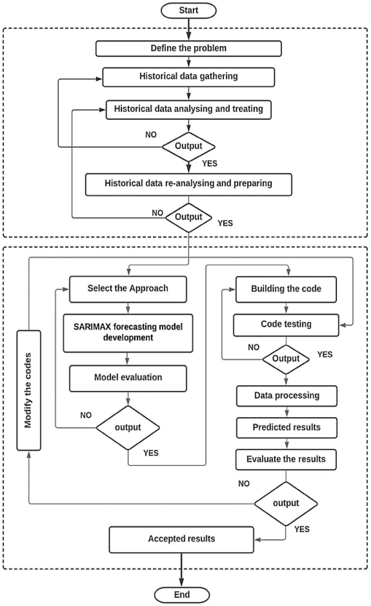
3. Materials and Methods

The ARIMA model is a statistical tool that provides complementary approaches for predicting future values in time series to obtain meaningful insights with random errors. Although exponential smoothing approaches are constructed for the trend and seasonality captured in the data, the ARIMA model describes autoregressive moving average linear model types in statistical predictions [39,40]. However, there is a significant stumbling block in the adoption of the ARIMA prediction model: the order selection procedure is often considered subjective and is difficult to implement [41]. The performance with seasonal series data renders the use of the standard ARIMA model ineffective [42]. The model has the disadvantage of not being able to handle seasonal data, which is frustrating. Thus, the ARIMA model was upgraded to the SARIMA model [43] to maintain the time series when it uses both seasonal and non-seasonal data for processing univariate time series data [42].
The main components of the ARIMA model are autoregression (AR), integration (I), and the moving average (MA), and the model defines the data as stationary, non-stationary, and seasonal processes with the order (p, d, q), where p refers to the autoregressive lag observations included in the model, d is the difference order or the number of times that the raw observations are differenced, and q is the MA lag or the size of the MA window [44]. The seasonal ARIMA p , d , q   *   P , D , Q s are the non-negative integers for handling seasonality, X t is the observed value at time t , and s is the number of periods per season. Equation (1) represents the general form of the SARIMA prediction model [45].
φ p G φ p G s   1 G d     1 G s D   X t = γ q G   w Q G s     e t  
where the coefficients φ p G and γ q G are the orders of the non-seasonal AR and non-seasonal MA components’ characteristic polynomials, and the polynomials φ p G s and   w Q G s are the seasonal autoregressive (SAR) and seasonal moving average (SMA) polynomials, respectively [45]. The non-seasonal and seasonal time series are 1 G and 1 G s , respectively, which are the differencing components. In addition, d and D are the non-seasonal ARIMA model’s ordinary differenced terms and the SARIMA model’s seasonal differenced terms, respectively; e t is the prediction error; s is the duration of the seasonal pattern (e.g., s = 12 monthly series); and G is the backshift operator coefficient. Equations (2)–(5) represent the SARIMA prediction model.
RA : φ p G = 1 φ 1 G φ 2 G 2 φ 3 G 3 φ p G p
MA : γ q G = 1 γ 1 G γ 2 G 2 γ 3 G 3 γ q G q
SRA : φ p G s = 1 φ 1 G s φ 2 G 2 s φ 3 G 3 s φ p G p s
SMA :   w Q G s = 1 w 1 G s w 2 G 2 s w 3 G 3 s w Q G Q s

3.1. Autoregressive Integrated Moving Average with Exogenous Factors (ARIMAX)

The ARIMAX prediction model is another version of the ARIMA model, which utilizes historical univariate time series data to analyze and predict trends and future values. The ARIMAX model has additional independent factors or explanatory variables compared with the ARIMA model, which were introduced to address the univariate time series issue. The ARIMAX model is a multiple regression model consisting of one or more AR terms and one or more MA terms. In addition, this model is suitable for any type of data pattern, such as stationary or non-stationary data and univariate data with trends. The model can be mathematically presented as shown in Equation (7) [46], where φ G refers to the AR parameters and γ G refers to the MA parameters. In addition, the regression error is e t ,   a t denotes a zero average and the time series error term, l i refers to the lag degree, and y t is the output.
e t   = γ G φ G   a t
y t = α + i = 1 m γ i ( G ) φ i ( G ) G l i X t + e t

3.2. Seasonal Autoregressive Integrated Moving Average with Exogenous Factors Model

The SARIMAX model is an improved version of the SARIMA model, with exogenous factors (X) as external feature parameters for enhancing the model’s performance, reducing the prediction errors, overcoming the autocorrelation issues, and improving the prediction results [45]. The SARIMAX model consists of both seasonal effects and exogenous factors that can be used as SARIMAX (p, d, q) ∗ (P, D, Q), while the exogenous factors are optional parameters. The exogenous factors can be external parallel time series data such as wind speed or temperature values that have the same correlation with the original data which need to be predicted. The exogenous factors are used to support the prediction model and to provide it with more details. The SARIMAX model can be presented as shown in Equation (8) [45], where y k , t refers to the number of external exogenous factors at time t and α k is the correlation coefficient value of the external exogenous input factors.
φ p G φ p G s   1 G d     1 G s D   X t = α k y k , t + γ q G   w Q G s     e t  

3.3. Autocorrelation (ACF) and Partial Autocorrelation (PACF)

The autocorrelation function (ACF) and the partial autocorrelation function (PACF) are fundamental tools for analyzing linear time series and are utilized to select the p and q values for the ARIMA model. Graphically, a correlogram shows how linearly related two pairs of observations are at different time lags, demonstrating how such pairs of observations are related to each other. In addition, the ACF and PACF can be used to identify models; fit autoregressive models; find periodicities, outliers, and category time series; and forecast future values [47]. When the ACF has values close to −1, the outliers will have the greatest influence or effect. When it has large positive values, a few successive outliers can enhance the prediction by offsetting and overcoming the small sample bias. However, some transformations can eliminate the impact of outliers on the ACF, although their biases persist asymptotically [47]. The PACF, on the other hand, provides an attractive vantage point for observing the structure of time series and also provides adequate criteria for a sequence of real numbers to describe weak stationary time series [48].

3.4. The Augmented Dickey–Fuller (ADF) Test and the Null Hypothesis

The augmented Dickey–Fuller (ADF) test can be used to determine whether a set of data is stationary or non-stationary [44,49]. In the case of non-stationary data, high-order differencing can be applied to make the data stationary [44]. ADF results are evaluated on the basis of two types of values: the statistic value and the p-value. A large negative statistic value leads to strong rejection of the unit root hypothesis, indicating that the time series has no unit root and thus is stationary. If the ADF test statistic result is positive, the null hypothesis of a unit root is not rejected, indicating that the time series has a unit root and thus is non-stationary. In addition, the ADF test generally involves the implementation of the null hypothesis to evaluate the data as stationary or non-stationary by denoting these as H 1 or H 0 [44]. H 1 refers to a time series that does not have a unit root; in this case, the null hypothesis is rejected, and the data are considered to be stationary [44]. H 0 , on the other hand, refers to a time series that has a unit root; in this case, the null hypothesis is not rejected and the data are considered to be non-stationary. The p-values that are used to decide between H 1 and H 0 are shown below.
  • If p ≤ 0.05, the mean time series does not contain a unit root, the null hypothesis is rejected, and the data are stationary [6,11].
  • If p > 0.05, the mean time series contains a unit root, the null hypothesis is not rejected, and the data are non-stationary [6,11].
Mathematically, the ADF test can be presented as shown in Equation (9), where α is a constant, β is a time trend parameter, γ and δ are coefficients, p is the AR process’s lag order, γ is the null hypothesis, y t is the dependent variable, and   y t is the first-difference operator.
  y t = α + β t + γ   y t 1   + δ 1   y t 1 + + δ p 1   y t p + 1 + e t  

3.5. Study Area and Data Collection

In this study, Saudi Arabia was selected as a case study. This country is located in western Asia and lies between latitudes 16° and 33° N and longitudes 34° and 56° E. Its historical energy data were collected from the King Abdullah Petroleum Studies and Research Center, the Saudi Water and Electricity Regulatory Authority, and U.S. Energy Information Administration [50,51]. They consisted of electricity generation, consumption, peak load, and installed capacity data, as presented in Figure 1, Figure 2, Figure 3 and Figure 4. The actual historical data pertained to quarterly intervals over a 40-year period (1981–2020) and were used to evaluate and predict the behavior of the power sector over a 30-year period (2021–2050). Furthermore, the quality of the historical data could provide details that could increase the SARIMAX model’s forecasting accuracy. The historical data were evaluated, validated, and cleaned to ensure that there were no missing or duplicate values. The Dickey–Fuller test revealed that the data were stationary, with p < 0.05.

3.6. Error Indices

Various indices were identified as common error indicators to comprehensively evaluate the proposed SARIMAX forecasting model’s efficiency. Moreover, modeling error indicators (mean square error (MSE), root mean square error (RMSE), mean absolute percentage error (MAPE), and mean absolute error (MAE)) were used to assess the model’s reliability and correctness, as mathematically shown in Equations (10)–(13), where the variable y j is the actual value, y ^ j refers to the forecasted observations, and ( n ) refers to the sample numbers used in the observation. Furthermore, the standard deviation of the regressions (the forecast error) is indicated by the term “RMSE”, which is the square root of the mean square errors and is recognized as an effective general-purpose error indicator for numerical predictions due to its low sensitivity to noise. In addition, the squared correlation coefficient (R2) indicates how much of a dependent variable’s fluctuation can be described by exogenous factors and how strong of a linear relationship there is between each two variables. In Equation (14), S S r e s is the sum of squared residuals and S S T o t is the absolute square number.
MSE = 1 n j = 1 n ( y j y ^ j ) 2      
RMSE = 1 n   j = 1 n   y j y ^ j   2 n
MAPE = 1 n j = 1 n     y j y ^ j   y j * 100
MAE = 1 n j = 1 n y j y ^ j  
R 2 = 1 SS res SS Tot

3.7. Model Setup and Configuration

Using Python programming, we developed a SARIMAX forecasting model based on the time series concepts, principles, and computational approaches presented in Equations (1)–(9). Python programming has a vast amount of memory, is capable of handling massive amounts of data, and has a wide range of prebuilt libraries. The datasets were prepared and cleaned in preparation for processing. Furthermore, due to the size and nature of the datasets, various parameter settings were necessary for each type of data to improve the model fit. To this end, we developed a method that automatically splits the training and testing data to match the model’s specifications. The total dataset length was 164 steps, and the data were divided into training and testing data, which accounted for 30% and 70% of all data, respectively. Furthermore, we developed a robust and effective code that monitors the performance of the model, generates an automatic report to identify any weak points in the code, defines the parameters (p, d, q) and (P, D, Q), and then automatically sets the values for the variables (p, d, q) to (1, 0, 6) and the orders (P, D, Q) to (3, 1, 1). In addition, the exogenous factors were set as 0. Many developers split the training and testing data manually and define the parameters of the variables randomly, which might result in incorrect values and negatively impact the model’s performance. Any unknown variables that might produce data fluctuations will make it impossible to predict them unless there is a known variable that explains the variations.
The flowchart of the proposed SARIMAX forecasting model is presented in Figure 5. In addition, Figure 5 summarizes the research process, which started with defining the problem, followed by data collection, data testing, and analysis. The process also included selecting the approach, developing the forecasting model, evaluating the forecasting model, and testing the final forecasting results.

4. Results and Discussion

The SARIMAX model was developed to forecast the future electricity generation, consumption, peak load, and installed capacity values in Saudi Arabia for a 30-year period (2021–2050) based on historical data collected over the previous 40 years. In addition, as energy demand rises, new dynamic energy markets emerge, which lead to an imbalance in energy prices and have a direct influence on the energy security of the world. These forecasting technologies present new opportunities for the energy market such as market developments, energy market performance, energy prices control, cost savings, and optimization that can solve obstacles for the businesses operating in this industry. Furthermore, help determine which energy markets provide the most opportunities for the power generation profile of the organization, minimizing the likelihood of grid congestion while simultaneously improving electricity flow. Moreover, the forecasting technologies are critical to ensure the stability of the energy system, since the efficiency of the energy markets is dependent on the availability of a dependable supply, flexible bidding, system assistance, predictive maintenance, and enhanced power quality. Forecasting is a challenging task because several confounding factors must be considered, such as the links between the regressors that have major effects on the power sector, as well as the intermittency and fluctuations, which cause apparent effects resulting from multiple errors. The developed model was used to forecast the future performance of the power sector in Saudi Arabia, as presented in Figure 6, Figure 7, Figure 8 and Figure 9. The estimates and findings showed that the SARIMAX model was able to properly handle the four types of electricity data as a multimodal dataset. The main and cross effects were evaluated by repeatedly plotting, analyzing, and testing the data. The electricity generation (Figure 6a), electricity consumption (Figure 7a), electricity peak load (Figure 8a), and installed power capacity (Figure 9a) data did not exhibit any significant overfitting between the experimental and forecasted values, indicating that the SARIMAX model has a promising performance with this type of historical data. Moreover, the model produced remarkable error metrics in terms of accuracy indicators, as shown in Table 1. The error metrics of electricity generation were as follows: RMSE = 1.2 TWh, MAE = 0.6 TWh, MSE = 1.5 TWh, and MAPE = 0.3%. Furthermore, electricity generation had an R2 of 99%. A reduction in the consumption RMSE to 1 TWh was achieved, but the MAE recorded the same value as the generation MAE (0.6 TWh) due to the similarity between the historical electricity consumption and generation data. The consumption MSE and MAPE were recorded as 1 TWh and 0.3%, respectively, with R2 = 99%. The MAPE values were influenced by the small values in the historical data. The peak load error indicators dropped, with RMSE = 0.3 GW, MAE = 0.1 GW, MSE = 0.1 GW, MAPE = 0.4%, and R2 = 99%. The error metric values for installed capacity were significantly smaller than the error values for electricity generation, consumption, and peak load. The error metrics for installed capacity showed significant improvements, with RMSE = 0.2 GW, MAE = 0.1 GW, MAPE = 0.3%, and R2 = 99%, as presented in Table 1. In addition, the MSE decreased to 0.07 GW. Although the MAPE is the most important measurement for predicting accuracy in the electrical forecasting literature, the MAE, MSE, and RMSE are also presented in this work. Applying different type of forecasting accuracy indicators has a significant and important role in evaluating the SARIMAX model. However, it is essential to carry out investigations on the question of whether or not the values of the four error metrics are consistent with each another.

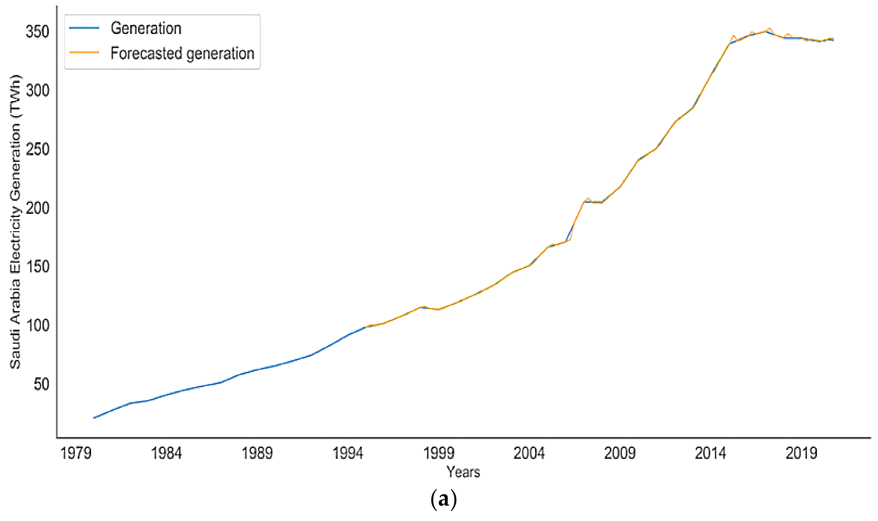
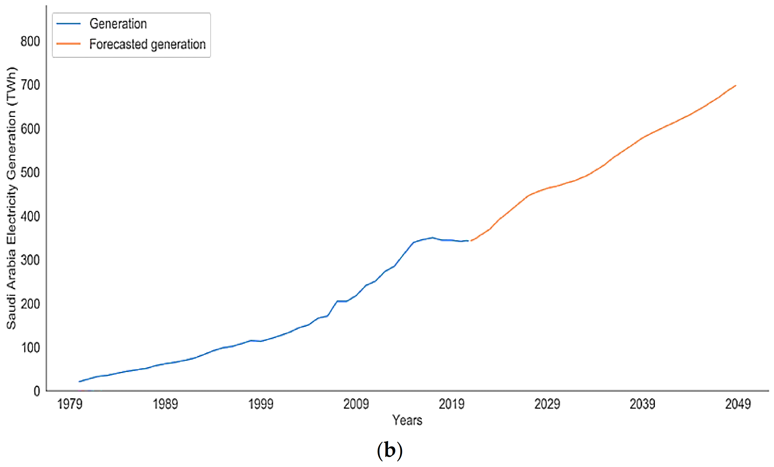
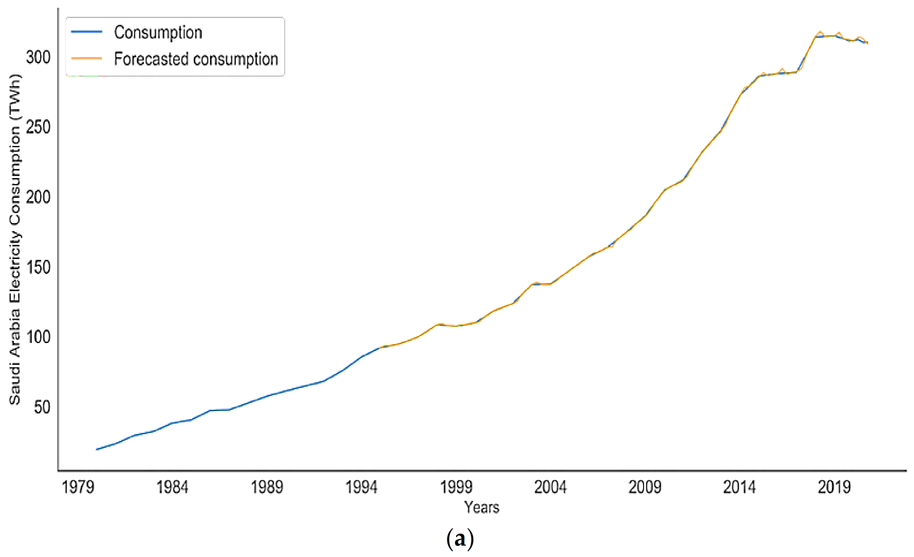
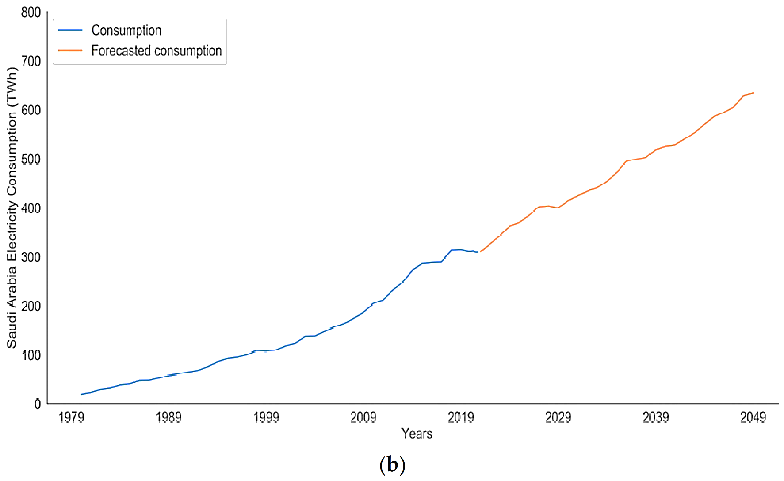
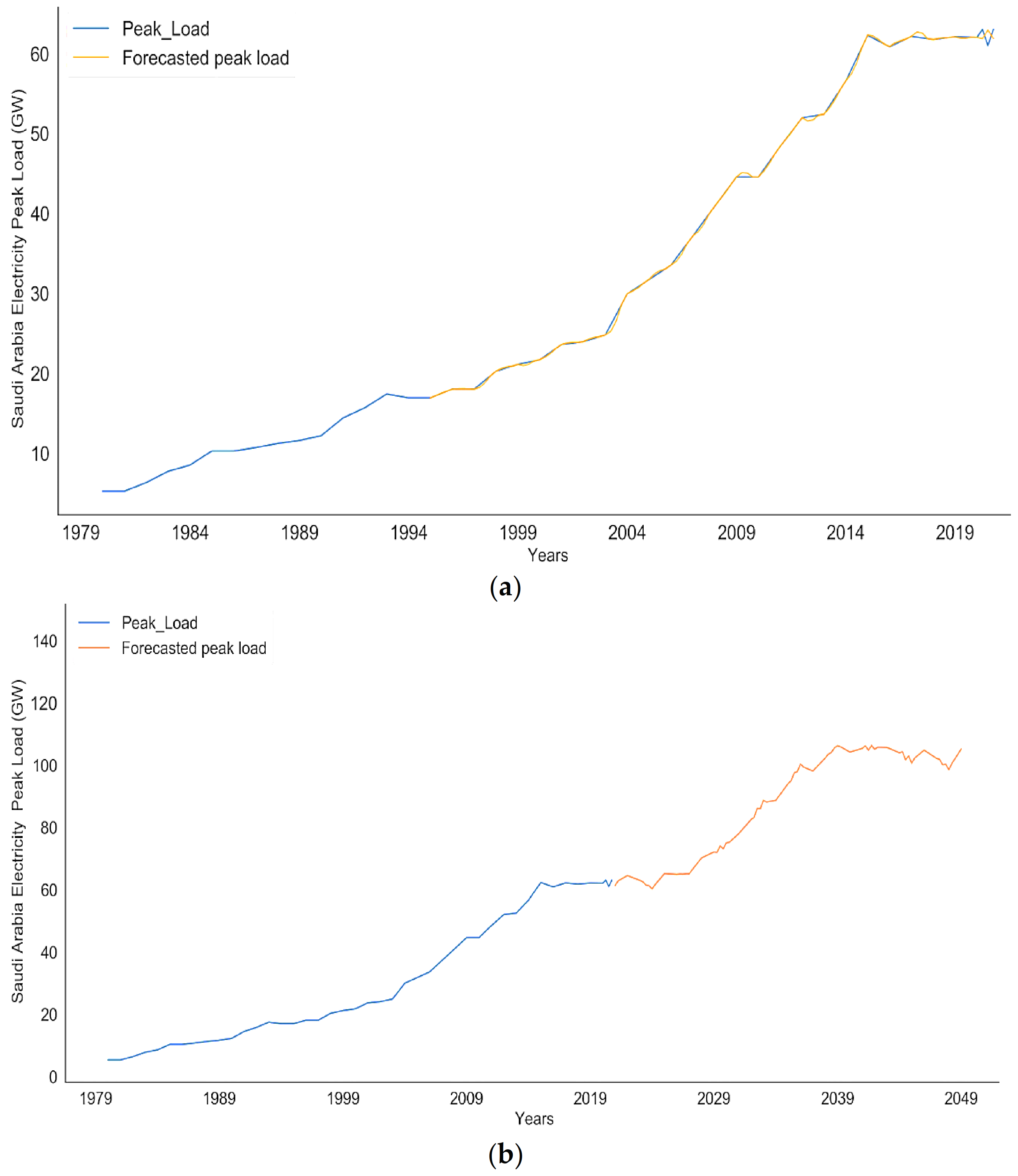
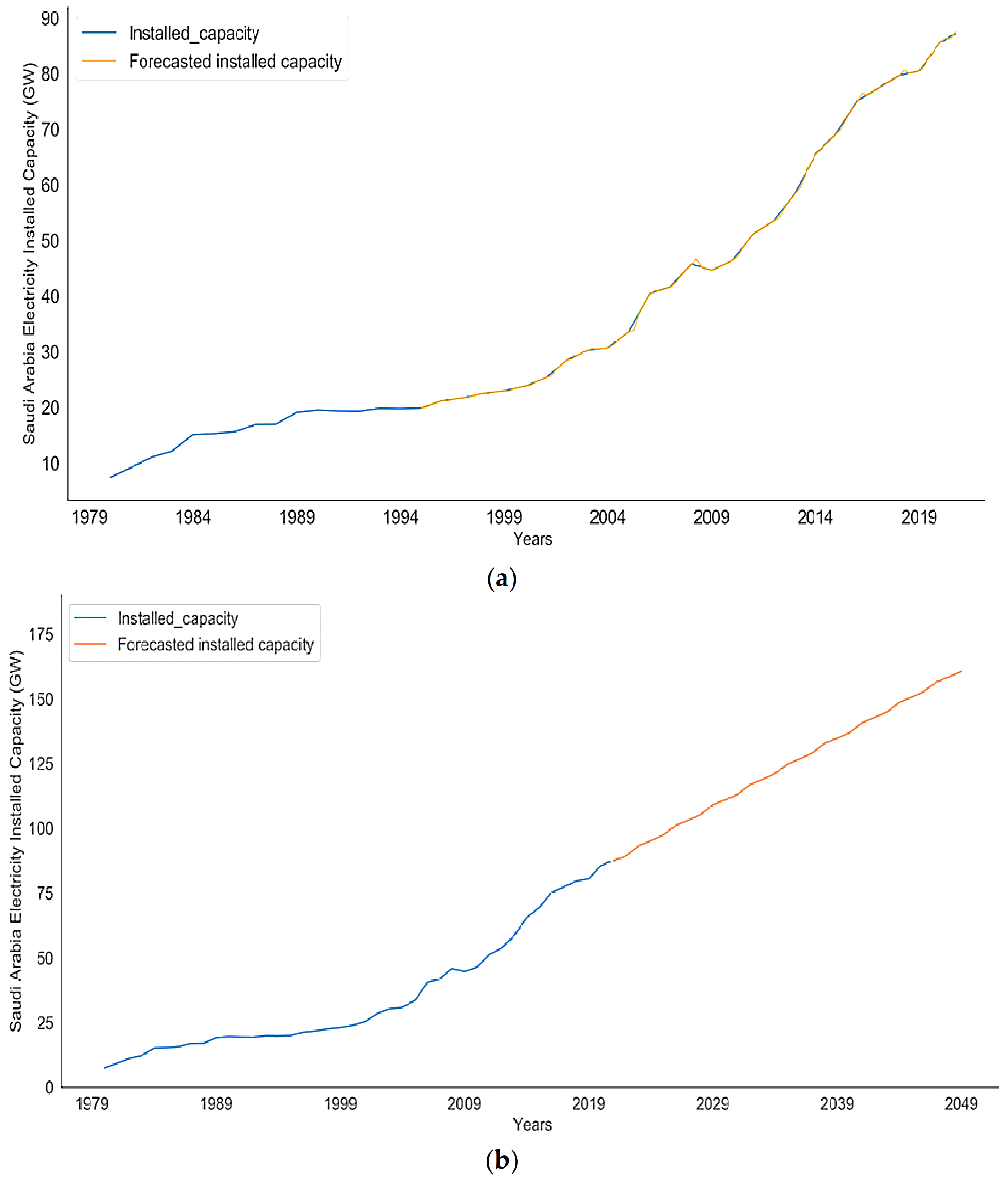
4.1. Future Performance Analysis for Saudi Arabia’s Electricity Sector

In addition, Figure 6b, Figure 7b, Figure 8b and Figure 9b illustrate the forecasted values of electricity generation, consumption, peak load, and installed capacity in Saudi Arabia for the 30-year period from 2021 to 2050. It is evident that among all the types of historical data, the historical peak load and installed capacity data values showed unique erroneous indicator values that decreased along with them (except for the MAPE value). This was caused by the unique nature of the historical electricity peak load and installed capacity data. Significant and acceptable correlations between the variables’ fluctuations in the four categories of historical power data were shown by the R2 values, indicating that the correlations were considerable and suitable. The statistical analysis of the historical power data and the SARIMAX forecasting results showed that electricity consumption is likely to continue growing at a swift rate until 2050, but the estimated electricity generation values were higher than the estimated electricity consumption values, although they were very close to each other (see Figure 6b and Figure 7b). The forecasted installed capacity values showed an increasing trend over the 30-year period from 2021 to 2050, which is reasonable for meeting the growth in electrical consumption. The electricity peak load did not show continuous growth because it depends on different factors, such as the weather and season. In general, the main factors that cause surges in electricity consumption and major variations in the electricity peak load are greenhouse gas emissions, changes in gross domestic product, and population growth. This demonstrates how crucial it is to include the cross effects into both short-term and the long-term forecasting models. In addition, evaluating the other external factors and their interconnections might further enhance the investigation and accuracy of forecasts.
According to Figure 6b, electricity generation in Saudi Arabia will be 369 TWh in 2023, and it was estimated to continue to increase to 409 TWh in 2025. Moreover, electricity generation will reach 470 TWh in 2030 and 516 TWh in 2035. In 2040, the electricity generation will be 589 TWh, and it will reach 643 TWh in 2045 and 700 TWh in 2050.
Figure 7b indicates that Saudi Arabia’s electricity consumption will reach 342 TWh in 2023 and will continue to rise to 373 TWh in 2025. In addition, the consumption of electricity will reach 421 TWh in 2030 and 483 TWh in 2035. In 2040, 524 TWh of electricity will be consumed, followed by 590 TWh in 2045 and 644 TWh in 2050. The increase in electricity consumption in Saudi Arabia has always been linked to three main factors, namely the increase in temperature that requires the use of air conditioners, especially in the summer, and the scarcity of water sources, which requires the use of seawater desalination plants. In addition, the large increase in the population as well as economic and urban growth affect electricity consumption.
The results of analyzing the future and historical data of electricity peak load in Saudi Arabia showed that the electricity peak load will reach 62 GW in 2023 and 66 GW in 2025, as presented in Figure 8b. Furthermore, the main reason for the fluctuation in the load values in Saudi Arabia is the increase in electrical loads at peak times, especially in the summer and official working hours, and during the month of Ramadan. Furthermore, the electricity peak load of Saudi Arabia is expected to reach 74 GW in 2030 and 94 GW in 2035. It is expected that the electricity peak load will be 103 GW in 2040, 104 GW in 2045, and 105 GW in 2050. In particular, the peak load grows in the summer to its highest level before falling to its lowest level in the winter (see Figure 8).
The installed electricity capacity of Saudi Arabia is continuing to rise to meet the requirements of the electrical industry in terms of electricity consumption. According to Figure 9b, the installed electrical capacity in Saudi Arabia will be 93 GW in 2023, and it is expected to continue increasing to 97 GW in 2025. In addition, the installed capacity will reach 110 GW in 2030, 124 GW in 2035, 136 GW in 2040, 150 GW in 2045, and 160 GW in 2050.

4.2. SARIMAX Model Evaluation

Eleven external models that predict long-term power consumption were selected to compare their performance with that of the proposed SARIMAX model based on the MAPE, RMSE, MAE, and MSE error metrics and R2. However, the authors of the study from which the forecasting models 5–11 originated used only two error metrics to evaluate their models (MAPE and RMSE) and did not provide the R2 values. The evaluation metrics of our proposed model were superior to those of the other external power consumption models (see Table 2). Moreover, the R2 of our SARIMAX model was 99% for our four types of historical data, which is higher than the R2 values of the external models. Based on the comparison in Table 2, machine learning and deep learning forecasting models perform worse than univariate time series forecasting. The comparison of the proposed SARIMAX model with the external models represents an added value to this paper, since it allowed us to evaluate our work independently and in relation to other works. Therefore, it is important that future studies use different tools and procedures to evaluate their work and compare it with published papers. This could be useful for researchers who are making predictions under similar conditions.
In addition, the forecasting performance of the SARIMAX model was checked at quarterly dataset intervals with different sizes of historical data and four types of historical data to test its forecasting accuracy under different conditions. Overall, all the SARIMAX model’s error values for the four types of historical data were minimal compared with those of the other forecasting models, proving the model’s adaptability to new historical data observations. Furthermore, the proposed model could easily cope with different types of historical data and generated promising forecasting results with very low error metrics in terms of accuracy and interpretability. The model’s performance is particularly impressive in terms of installed power capacity. The error values also decreased, and the training time increased. Furthermore, the integration of a substantial quantity of historical data with a sizable amount of training data further extended the duration of the simulation. However, because of the interdependence of the succeeding phases, the SARIMAX prediction model must be treated sequentially. The most difficult tasks are strengthening the generalization capabilities of the model while simultaneously attaining better outcomes. Generalization is described as the fluctuation in the recognition rate of the model’s performance when matching the training data to previously observed datasets, such as the testing data. The model lacked generalization results because of the significant overfitting of the training and testing data, but it did not exhibit significant overfitting Figure 6a, Figure 7a, Figure 8a and Figure 9a. The SARIMAX model incorporates time series to improve its generalization by considering the effects of the parameters on the expected historical data values for the next step. When a significant number of sufficient historical data are selected, the SARIMAX model’s efficiency becomes evident, its long-term forecasting quality improves, and its accuracy increases. In this study, the most appropriate method and the best approach for long-term forecasting—a time series—was developed. The method considered trends and seasonal effects (summer, winter and spring), which provided the SARIMAX model with more details for understanding the input data and improving performance. Furthermore, the method considered the null hypothesis requirements for stationary data. Moreover, a code that automatically divides the training and testing data was developed to meet the requirements of the model as 30% for training and 70% for testing. However, even after selecting the most suitable forecasting method, it is essential to monitor forecasting accuracy continuously.
In this study, we used several error metrics to evaluate our proposed model and to provide other model developers with more options for comparing their work using these error metrics. We also aimed to provide future research with guidelines and a roadmap based on our experimental findings. This study could provide solid alternative procedures for future research by emphasizing the importance of the time series approach and how to choose the most appropriate forecasting technique for long-term forecasts, such as for the next 30 years.

5. Conclusions

This study helped fill the knowledge gaps in long-term electricity sector forecasting by developing a long-term forecasting model that considers the implications of electricity generation, consumption, peak load, and installed capacity for future performance analyses and in planning to address the fluctuation and uncertainty issues that can impact the stability of the power system and the energy markets. In addition, enhancing the quality of the power system will have a major effect on the scheduling, operation, and integration of energy. Moreover, the forecasting model can be used to enhance the efficiency of the energy markets. Therefore, applying forecasting techniques and paradigms can improve the performance of the energy markets, which is especially useful when there is uncertainty in the electricity markets. These forecasting models provide robust methodological approaches to crucial challenges pertaining to unpredictability in the electricity markets and to improving the microeconomics, energy policies, and evolution of global energy markets.
In this study, the SARIMAX forecasting model was developed and validated using a variety of selected features, including the time series algorithm and hypotheses regarding the most effective forecasting sequence and processes for the future performance of the power sector. The present research provides evidence that classical approaches are superior to the complex methods such as decision trees, multilayer perceptrons (MLP), LSTM neural network models and other deep learning methods, at least for the challenges investigated. Our experimental findings strongly encourage the use of classical models, such as SARIMAX. We emphasize the need for not only carefully using model preparation strategies but also actively testing several combinations of models and data preparation schemes for a particular situation to determine which method is the most effective. In addition, the most important issue and greatest difficulty is improving their accuracy and maximizing their vast potential. The model was evaluated and validated using four different types of historical electricity sector data: electricity generation, consumption, peak load, and installed capacity. The historical data covered 40 years (1980–2020) and were gathered from Saudi Arabia as quarterly interval data for forecasting the aforementioned values over the 30-year period from 2021 to 2050.
The SARIMAX forecasting model demonstrated the ability to cope with a variety of historical data types. The model’s effectiveness was tested using error indices, such as the RMSE, MAE, MSE, and MAPE values and the R2, as presented in Table 1. The highest RMSE value for the four types of electricity data was 1.2 TWh for electricity generation, and the lowest was 0.2 GW for installed capacity. The largest MAE value was 0.6 TWh for both electricity generation and consumption, and the lowest was 0.1 MW for both peak load and installed capacity. The MSE values ranged from 1.5 TWh for electricity generation to 0.07 GW for installed capacity. The MAPE values varied from 0.4% for peak load to 0.3% for all the other categories, and the R2 value was 99% for all four categories. As shown in Table 2, the comparison of the proposed SARIMAX model with 11 external prediction models strengthened our findings and validated the SARIMAX model’s performance, making a significant contribution to the literature by allowing us to analyze our work independently and with respect to other research.
The study findings also revealed that the SARIMAX model outperformed its competitors in terms of forecasting accuracy, overfitting, redundancy elimination, training time, and testing execution time, proving that it has remarkable performance. However, the model can be further improved, and its error indications can be reduced by improving the learning performance, optimizing the parameters, using monthly historical interval datasets, and adjusting the duration of the iterations.

The Importance of This Work and Future Research

This article discusses the importance of developing a long-term electricity energy forecasting method, such as the SARIMAX model, based on the time series approach. One of its contributions is narrowing the gap and addressing the existing deficiencies of time series methods, thus minimizing potential inconsistencies in energy forecasting. Through this study, we propose a long-term promising forecasting model and provide guidelines for future research.
In addition, there is a lack of feasibility studies on solar and wind energy, which are necessary for implementing renewable energy sources and diversifying the energy mix. In the future, we plan to improve and extend the SARIMAX model to forecast wind speed and solar radiation in several regions using historical data from the previous 35 years.

Author Contributions

F.R.A. performed the study and designed the model and the methodology. F.R.A. gathered the data, ran the software simulations, analyzed the results, and wrote the original draft. F.R.A. also reviewed the related previous research. D.C. supervised all the work, designed the procedure, and reviewed this manuscript step by step. D.C. reviewed, edited, and validated the results. D.C. visualized and improved the quality of this study. All authors have read and agreed to the published version of the manuscript.

Funding

This research received no external funding.

Institutional Review Board Statement

Not applicable.

Informed Consent Statement

Not applicable.

Data Availability Statement

Not applicable.

Conflicts of Interest

The authors declare no conflict of interest.

References

  1. Alsharif, M.H.; Younes, M.K.; Kim, J. Time series ARIMA model for prediction of daily and monthly average global solar radiation: The case study of Seoul, South Korea. Symmetry 2019, 11, 240. [Google Scholar] [CrossRef] [Green Version]
  2. Alharbi, F.R.; Csala, D. Short-Term Solar Irradiance Forecasting Model Based on Bidirectional Long Short-Term Memory Deep Learning. In Proceedings of the 2021 International Conference on Electrical, Communication, and Computer Engineering (ICECCE), Kuala Lumpur, Malaysia, 12–13 June 2021; pp. 1–6. [Google Scholar]
  3. Funahashi, K.-i.; Nakamura, Y. Approximation of dynamical systems by continuous time recurrent neural networks. Neural Netw. 1993, 6, 801–806. [Google Scholar] [CrossRef]
  4. Alharbi, F.R.; Csala, D. Short-Term Wind Speed and Temperature Forecasting Model Based on Gated Recurrent Unit Neural Networks. In Proceedings of the 2021 3rd Global Power, Energy and Communication Conference (GPECOM), Antalya, Turkey, 5–8 October 2021; pp. 142–147. [Google Scholar]
  5. Krizhevsky, A.; Sutskever, I.; Hinton, G.E. Imagenet classification with deep convolutional neural networks. Commun. ACM 2017, 60, 84–90. [Google Scholar] [CrossRef] [Green Version]
  6. Alharbi, F.R.; Csala, D. Wind Speed and Solar Irradiance Prediction Using a Bidirectional Long Short-Term Memory Model Based on Neural Networks. Energies 2021, 14, 6501. [Google Scholar] [CrossRef]
  7. Zhao, Y.; Ye, L.; Li, Z.; Song, X.; Lang, Y.; Su, J. A novel bidirectional mechanism based on time series model for wind power forecasting. Appl. Energy 2016, 177, 793–803. [Google Scholar] [CrossRef]
  8. Vu, D.H.; Muttaqi, K.M.; Agalgaonkar, A.P. Short-term load forecasting using regression based moving windows with adjustable window-sizes. In Proceedings of the 2014 IEEE Industry Application Society Annual Meeting, Vancouver, BC, Canada, 5–9 October 2014; pp. 1–8. [Google Scholar]
  9. Papalexopoulos, A.D.; Hesterberg, T.C. A regression-based approach to short-term system load forecasting. IEEE Trans. Power Syst. 1990, 5, 1535–1547. [Google Scholar] [CrossRef]
  10. Jain, R.K.; Smith, K.M.; Culligan, P.J.; Taylor, J.E. Forecasting energy consumption of multi-family residential buildings using support vector regression: Investigating the impact of temporal and spatial monitoring granularity on performance accuracy. Appl. Energy 2014, 123, 168–178. [Google Scholar] [CrossRef]
  11. Fan, C.; Xiao, F.; Wang, S. Development of prediction models for next-day building energy consumption and peak power demand using data mining techniques. Appl. Energy 2014, 127, 1–10. [Google Scholar] [CrossRef]
  12. Lee, C.-M.; Ko, C.-N. Short-term load forecasting using lifting scheme and ARIMA models. Expert Syst. Appl. 2011, 38, 5902–5911. [Google Scholar] [CrossRef]
  13. Yun, K.; Luck, R.; Mago, P.J.; Cho, H. Building hourly thermal load prediction using an indexed ARX model. Energy Build. 2012, 54, 225–233. [Google Scholar] [CrossRef]
  14. Liu, N.; Babushkin, V.; Afshari, A. Short-term forecasting of temperature driven electricity load using time series and neural network model. J. Clean Energy Technol. 2014, 2, 327–331. [Google Scholar] [CrossRef] [Green Version]
  15. Fan, G.-F.; Yu, M.; Dong, S.-Q.; Yeh, Y.-H.; Hong, W.-C. Forecasting short-term electricity load using hybrid support vector regression with grey catastrophe and random forest modeling. Util. Policy 2021, 73, 101294. [Google Scholar] [CrossRef]
  16. Papadopoulos, S.; Karakatsanis, I. Short-term electricity load forecasting using time series and ensemble learning methods. In Proceedings of the 2015 IEEE Power and Energy Conference at Illinois (PECI), Champaign, IL, USA, 20–21 February 2015; pp. 1–6. [Google Scholar]
  17. Xie, M.; Sandels, C.; Zhu, K.; Nordström, L. A seasonal ARIMA model with exogenous variables for elspot electricity prices in Sweden. In Proceedings of the 2013 10th International Conference on the European Energy Market (EEM), Stockholm, Sweden, 27–31 May 2013; pp. 1–4. [Google Scholar]
  18. Box, G.E.P.; Jenkins, G.M.; Reinsel, G.C.; Ljung, G.M. Time Series Analysis: Forecasting and Control; John Wiley & Sons: Hoboken, NJ, USA, 2015. [Google Scholar]
  19. Cai, M.; Pipattanasomporn, M.; Rahman, S. Day-ahead building-level load forecasts using deep learning vs. traditional time-series techniques. Appl. Energy 2019, 236, 1078–1088. [Google Scholar] [CrossRef]
  20. Vagropoulos, S.I.; Chouliaras, G.I.; Kardakos, E.G.; Simoglou, C.K.; Bakirtzis, A.G. Comparison of SARIMAX, SARIMA, modified SARIMA and ANN-based models for short-term PV generation forecasting. In Proceedings of the 2016 IEEE International Energy Conference (ENERGYCON), Leuven, Belgium, 4–8 April 2016; pp. 1–6. [Google Scholar]
  21. Sheng, F.; Jia, L. Short-term load forecasting based on SARIMAX-LSTM. In Proceedings of the 2020 5th International Conference on Power and Renewable Energy (ICPRE), Shanghai, China, 12–14 September 2020; pp. 90–94. [Google Scholar]
  22. Alasali, F.; Nusair, K.; Alhmoud, L.; Zarour, E. Impact of the covid-19 pandemic on electricity demand and load forecasting. Sustainability 2021, 13, 1435. [Google Scholar] [CrossRef]
  23. Sutthichaimethee, P.; Ariyasajjakorn, D. Forecasting energy consumption in short-term and long-term period by using arimax model in the construction and materials sector in thailand. J. Ecol. Eng. 2017, 18, 52–59. [Google Scholar] [CrossRef]
  24. Sutthichaimethee, P.; Naluang, S. The efficiency of the sustainable development policy for energy consumption under environmental law in Thailand: Adapting the SEM-VARIMAX model. Energies 2019, 12, 3092. [Google Scholar] [CrossRef] [Green Version]
  25. Elamin, N.; Fukushige, M. Modeling and forecasting hourly electricity demand by SARIMAX with interactions. Energy 2018, 165, 257–268. [Google Scholar] [CrossRef]
  26. Lee, J.; Cho, Y. National-scale electricity peak load forecasting: Traditional, machine learning, or hybrid model? Energy 2022, 239, 122366. [Google Scholar] [CrossRef]
  27. Tarsitano, A.; Amerise, I.L. Short-term load forecasting using a two-stage sarimax model. Energy 2017, 133, 108–114. [Google Scholar] [CrossRef]
  28. Bennett, C.; Stewart, R.A.; Lu, J. Autoregressive with exogenous variables and neural network short-term load forecast models for residential low voltage distribution networks. Energies 2014, 7, 2938–2960. [Google Scholar] [CrossRef]
  29. Soares, L.J.; Medeiros, M.C. Modeling and forecasting short-term electricity load: A comparison of methods with an application to Brazilian data. Int. J. Forecast. 2008, 24, 630–644. [Google Scholar] [CrossRef]
  30. Mohamed, N.; Ahmad, M.H.; Ismail, Z. Improving Short Term Load Forecasting Using Double Seasonal Arima Model. 2011. Available online: https://citeseerx.ist.psu.edu/viewdoc/summary?doi=10.1.1.389.5120 (accessed on 1 September 2022).
  31. Kim, M.S. Modeling special-day effects for forecasting intraday electricity demand. Eur. J. Oper. Res. 2013, 230, 170–180. [Google Scholar] [CrossRef]
  32. Alharbi, F.; Csala, D. Saudi Arabia’s solar and wind energy penetration: Future performance and requirements. Energies 2020, 13, 588. [Google Scholar] [CrossRef] [Green Version]
  33. Yu, F.; Xu, X. A short-term load forecasting model of natural gas based on optimized genetic algorithm and improved BP neural network. Appl. Energy 2014, 134, 102–113. [Google Scholar] [CrossRef]
  34. Caponetto, R.; Fortuna, L.; Graziani, S.; Xibilia, M.G. Genetic algorithms and applications in system engineering: A survey. Trans. Inst. Meas. Control. 1993, 15, 143–156. [Google Scholar] [CrossRef]
  35. Al Harbi, F.; Csala, D. Saudi Arabia’s Electricity: Energy Supply and Demand Future Challenges. In Proceedings of the 2019 1st Global Power, Energy and Communication Conference (GPECOM), Nevsehir, Turkey, 12–15 June 2019; pp. 467–472. [Google Scholar]
  36. Chen, Y.; Xu, P.; Chu, Y.; Li, W.; Wu, Y.; Ni, L.; Bao, Y.; Wang, K. Short-term electrical load forecasting using the Support Vector Regression (SVR) model to calculate the demand response baseline for office buildings. Appl. Energy 2017, 195, 659–670. [Google Scholar] [CrossRef]
  37. Zhang, J.; Wei, Y.-M.; Li, D.; Tan, Z.; Zhou, J. Short term electricity load forecasting using a hybrid model. Energy 2018, 158, 774–781. [Google Scholar] [CrossRef]
  38. Bucolo, M.; Fortuna, L.; Nelke, M.; Rizzo, A.; Sciacca, T. Prediction models for the corrosion phenomena in Pulp & Paper plant. Control. Eng. Pract. 2002, 10, 227–237. [Google Scholar]
  39. Ampountolas, A. Modeling and Forecasting Daily Hotel Demand: A Comparison Based on SARIMAX, Neural Networks, and GARCH Models. Forecasting 2021, 3, 580–595. [Google Scholar] [CrossRef]
  40. Barrow, D.; Kourentzes, N. The impact of special days in call arrivals forecasting: A neural network approach to modelling special days. Eur. J. Oper. Res. 2018, 264, 967–977. [Google Scholar] [CrossRef] [Green Version]
  41. Hyndman, R.J.; Athanasopoulos, G. Forecasting: Principles and Practice; OTexts: Melbourne, Australia, 2018. [Google Scholar]
  42. Papaioannou, G.P.; Dikaiakos, C.; Dramountanis, A.; Papaioannou, P.G. Analysis and modeling for short-to medium-term load forecasting using a hybrid manifold learning principal component model and comparison with classical statistical models (SARIMAX, Exponential Smoothing) and artificial intelligence models (ANN, SVM): The case of Greek electricity market. Energies 2016, 9, 635. [Google Scholar]
  43. Makridakis, S.; Wheelwright, S.C.; Hyndman, R.J. Forecasting Methods and Applications; John wiley & sons: Paphos, Cyprus, 2008. [Google Scholar]
  44. Naik, K. Hands-On Python for Finance: A Practical Guide to Implementing Financial Analysis Strategies Using Python; Packt Publishing Ltd.: Birmingham, UK, 2019; p. 378. [Google Scholar]
  45. Manigandan, P.; Alam, M.D.; Alharthi, M.; Khan, U.; Alagirisamy, K.; Pachiyappan, D.; Rehman, A. Forecasting Natural Gas Production and Consumption in United States-Evidence from SARIMA and SARIMAX Models. Energies 2021, 14, 6021. [Google Scholar] [CrossRef]
  46. Bierens, H.J. ARMAX model specification testing, with an application to unemployment in the Netherlands. J. Econom. 1987, 35, 161–190. [Google Scholar] [CrossRef]
  47. Dürre, A.; Fried, R.; Liboschik, T. Robust estimation of (partial) autocorrelation. Wiley Interdiscip. Rev. Comput. Stat. 2015, 7, 205–222. [Google Scholar] [CrossRef]
  48. Ramsey, F.L. Characterization of the partial autocorrelation function. Ann. Stat. 1974, 1296–1301. [Google Scholar] [CrossRef]
  49. Bengtsson, E.; Påhlman, S. The Effect of Rising Interest Rates on Swedish Condominium Prices. Bachelor’s Thesis, University of Gothenburg, Gothenburg, Sweden, 2021. [Google Scholar]
  50. Independent Statistics & Analysis-U.S. Energy Information Administration (EIA). Available online: https://www.eia.gov/international/data/world#/?pa=0000002&c=4100000002000060000000000000g000200000000000000001&tl_id=2-A&vs=INTL.2-2-AFRC-BKWH.A&vo=0&v=H&end=2016 (accessed on 25 August 2020).
  51. Alharbi, F.R.; Csala, D. GCC countries’ renewable energy penetration and the progress of their energy sector projects. IEEE Access 2020, 8, 211986–212002. [Google Scholar] [CrossRef]
Figure 1. Historical levels of electricity generation in Saudi Arabia.
Inventions 07 00094 g001
Figure 2. Historical levels of electricity consumption in Saudi Arabia.
Inventions 07 00094 g002
Figure 3. Historical levels of the electricity peak load in Saudi Arabia.
Inventions 07 00094 g003
Figure 4. Historical levels of electricity installed capacity in Saudi Arabia.
Inventions 07 00094 g004
Figure 5. Flowchart of the proposed SARIMAX forecasting model.
Inventions 07 00094 g005
Figure 6. (a) Real and forecasted values of electricity generation, which show the good fit and performance of the SARIMAX model. (b) Forecasted electricity generation values for the 30-year period from 2021 to 2050.
Inventions 07 00094 g006aInventions 07 00094 g006b
Figure 7. (a) Real and forecasted values of electricity consumption, which show the good fit and performance of the SARIMAX model. (b) Forecasted electricity consumption values for the 30-year period from 2021 to 2050.
Inventions 07 00094 g007aInventions 07 00094 g007b
Figure 8. (a) Real and forecasted values of the electricity peak load, which show the good fit and performance of the SARIMAX model. (b) Forecasted peak electricity load values for the 30-year period from 2021 to 2050.
Inventions 07 00094 g008
Figure 9. (a) Real and forecasted values of the installed electricity capacity, which show the good fit and performance of the SARIMAX model. (b) Forecasted electricity installed capacity values for the 30-year period from 2021 to 2050.
Inventions 07 00094 g009
Table 1. Forecasting accuracy indicators for the proposed SARIMAX model.
No.MetricGeneration
(TWh)
Consumption
(TWh)
Electric Peak Load (GW)Installed Capacity
(GW)
1RMSE1.210.30.2
2MAE0.60.60.10.1
3MSE1.510.10.07
4MAPE (%)0.30.30.40.3
5p-value (%)3 × 10−72 × 10−800
6R2 (%)99999999
Table 2. Comparison of the performance of the proposed SARIMAX model and external models.
No.Forecasting ModelMAPE (%)RMSE (GW) MAE (GW)MSE (GW)R2 (%)
1SARIMAX [26]5.424298.653614.0318,478.3979.60
2LSTM [26]2.983106.642027.579651.2486.10
3ANN [26]4.974109.633562.2416,889.1281.80
4SVR [26]4.163615.723004.1913,073.4382.20
5MLR model [24]20.0622.91---
6BP model [24]13.5016.87---
7Grey model [24]12.1114.48---
8ANN model [24]8.6510.15---
9ANFIS model [24]6.426.89---
10ARIMA model [24]6.293.41---
11SEM-VARIMAX model [24]1.061.19---
12SARIMAX proposed model0.3010.60199
Publisher’s Note: MDPI stays neutral with regard to jurisdictional claims in published maps and institutional affiliations.

