

Gradient Heatmetry in a Burners Adjustment
by
 ,
,
Pavel G. Bobylev
*,
Andrey V. Pavlov
,
Vyacheslav M. Proskurin
,
Yuriy V. Andreyev
,
Vladimir Yu. Mityakov
and
Sergey Z. Sapozhnikov
Science Educational Center “Energy Thermophysics”, Peter the Great St. Petersburg Polytechnic University (SPbPU), St. Petersburg 195251, Russia
*
Author to whom correspondence should be addressed.
Inventions 2022, 7(4), 122; https://doi.org/10.3390/inventions7040122
Submission received: 15 November 2022
/
Revised: 5 December 2022
/
Accepted: 9 December 2022
/
Published: 13 December 2022
(This article belongs to the Special Issue Thermodynamic and Technical Analysis for Sustainability (Volume 2))
Abstract
:Measuring the heat flux in the furnace of industrial boilers is an urgent task in the power industry. Installing the measuring instruments directly into the furnace is a laborious and complex process. It requires a complete shutdown of the boiler, which incurs economic costs. It is most efficient to use portable probes with measuring insert. The created cooled probe with a heterogeneous gradient heat flux sensor is a unique and versatile tool that allows for the configuration and control of the operation of power boilers. This article compares experimental values with calculation methods. The obtained heat flux per unit area is in good agreement with the theoretical concepts when the values are averaged. The technique used in this paper makese it possible to determine the maximum heat-stressed zones and areas with stable or unstable combustion. The main combustion zones that are typical for the flaring of any fuel are identified. This approach allows us to consider various approaches to heat transfer enhancement during the combustion of both liquid and gaseous fuels. Comparison of experimental results with the data of other authors is not quite exact due to the complexity of the experiment. The study of burners in this configuration has not previously been considered in the literature.
1. Introduction
Uneven heat generation and flame instability depend on many factors, for example, the guiding device, oxidant supply system, fuel supply system malfunctions, etc. Power equipment time lag leads to difficulty in identifying problems with the burner as they arise. Generally, two sensors control the operation of the burner: the flame sensor and the fuel flow rate meter. Their data make it possible to analyse burner malfunctions only in cases of emergency, and it is impossible to detect the origin of malfunction.
Differences in boiler equipment design features makes monitoring more complicated. In fire-tube boilers, irregularity of heat generation, unstable flame, etc., can cause burnout of the fire tube, which is fatal for the entire power plant. Usually, boilers of this type are low-power and have one burner, which makes them easier to control. In high-power water-tube boilers with several burners, it is impossible to monitor the malfunction of each burner.
Currently, there is no methodology for calculating local heat generation from the flame. All functional connections have the form [1,2]:
where Q (W, watts) is the heat generated by fuel combustion, (kg/s) is the fuel mass flow rate, and (J/kg) is the fuel lower heating value.
The dependence on (1) makes it possible to estimate the average heat generation during fuel combustion only, not the distribution of the flame local heat flux. Most experiments and practical monitoring of thermal equipment have been conducted using temperature measurement. In spite of the need to measure the heat flux per unit area and not the temperature, there are significantly fewer primary converters for measuring heat flux than invasive and non-invasive thermal sensors.
The most interesting and valuable paper in this regard is the investigation by D. Zhang et al. [3], where a probe for measuring the heat flux from a flame was presented. As stated above, its principle of operation is based on temperature measurement. The measuring insert has the form of a solid cylinder with two thermocouples mounted on the cylinder axis. For this design, the probe sensitivity is determined by the temperature difference. With an increase in the distance between the thermocouples, the sensitivity increases, while the response time decreases. In accordance with the obtained data, the authors identified an optimal distance for the experimental conditions of 8 mm. This probe made it possible to consider the heat generated from the torch in the furnace of a 600 MW supercritical arch-fired boiler (SC-AFB). Measurement of the heat flux in aggressive media can be performed using sensors which are a set of thermocouples [3].
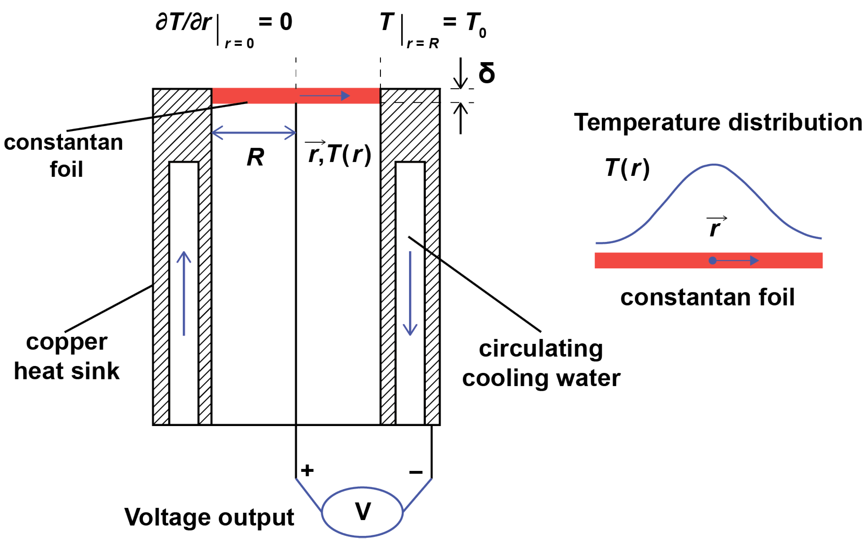
Another common way to measure heat flux from a flame is to use a diffusion-type Gardon Gauge. Its application in combustion is good, as shown in [4]. The design of the sensor is shown in Figure 1. It consists of a thin piece of circular constantan foil attached to a massive copper radiator, which is the sensor housing.
The copper conductor is attached to the center of the foil, forming one copper-constantan (T-type) thermocouple at the junction. The second connection is formed along the edges of the constantan disk, at the point of contact with the copper radiator.
Thermal radiation moves evenly downwards at the surface of the constantan disk, which is a sensitive element. As a result, it is radially transferred to a copper radiator, which is kept cool by an internal cooling circuit by cold water. Thus, the temperature difference between the center and periphery of the disk is determined, followed by calculation of the heat flux. The Gardon Gauge has proven itself well in various fields, including measurement of heat flux in furnaces of power boilers and industrial furnaces [5], measurements of concentrated solar radiation [6], studies of heat transfer during the entry of spacecraft at hypersonic velocity into the Earth’s atmosphere [4], and more.
Sensors based on hyperthermocouples [4,7,8,9,10,11] are widely used in the study of heat transfer processes; however, they have an unavoidable drawback. The disadvantage in this case is their thickness, which is related to both sensitivity and response time. This article discusses an experimental probe that uses a gradient heat flux sensor (GHFS), which has a radically different principle of operation.
2. Experimental Procedure
2.1. Gradient Heatmetry
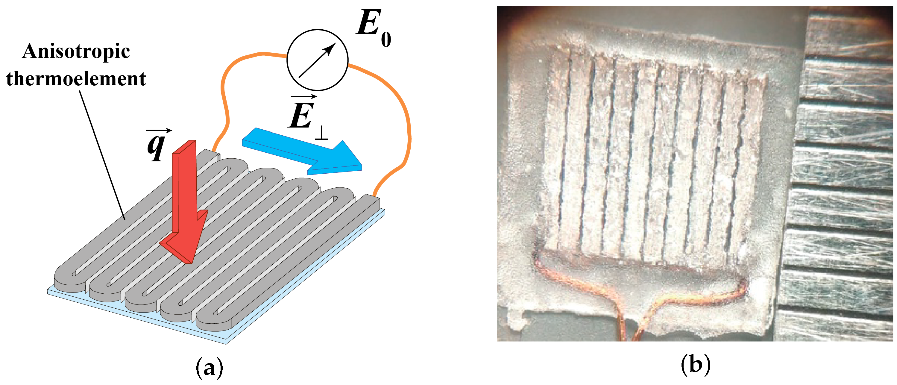
Gradient heatmetry is an innovative research method based on the use of gradient heat flux sensors (GHFS). These sensors are made of materials with thermal conductivity, electrical conductivity, and thermo-EMF coefficient anisotropy. Such materials are called anisotropic thermopower elements (ATE). Due to the fact that the GHFS is made of ATE, sensor operation is based on the transverse Seebeck effect; when affected by heat flux, GHFS generates thermo-EMF normally with respect to the heat flux per unit area vector and proportionally to the heat flux rate (Figure 2a). Mathematically, the relationship between the heat flux and the generated thermo-EMF is expressed by
where is the thermo-EMF (mV), is the GHFS volt-watt sensitivity (mV/W), A is the GHFS plan-area (m), and q is the heat flux (W/m). The volt-watt sensitivity is determined by the thermo-EMF and conductivity tensor components, as well as by the ATE width. Furthermore, there is maximum volt-watt sensitivity which can be achieved by optimally angular deflection of the ATE trigonal plane [12].
To estimate the sensitivity, GHFSs should be calibrated in an operational temperature range determined based on the individual experiment. When calibrating, it is necessary to obtain the dependence of the volt-watt sensitivity at temperature . GHFS are calibrated on special benches [12].
There are several methods of GHFS construction. Battery GHFS are made on the basis of 0.9999-purity single-crystal bismuth (Figure 2), which has natural anisotropic properties [13].
Despite the high (about 5…10 mV/W) volt-watt sensitivity and fast response time (10 s), a bismuth-based GHFS has a low temperature limit not exceeding the melting point of bismuth (544 K) [15].
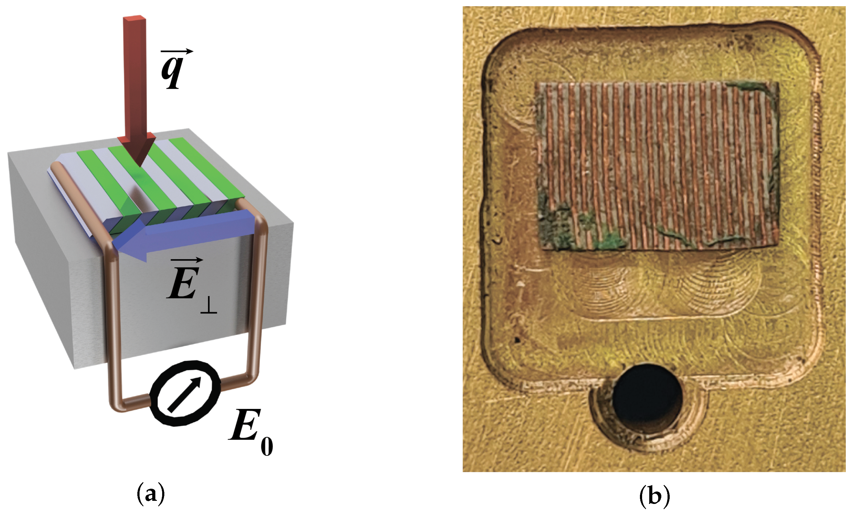
In 2007, researchers at Peter the Great St. Petersburg Polytechnic University created synthetic GHFS based on layered composites of metals, alloys, and semiconductors [14]. These are referred to as heterogeneous gradient heat flux sensors (HGHFS) (Figure 3).
Sensors of this type demonstrate high temperature limits (up to 1300 K); esentially, the composite is a synthetic anisotropic single crystal. Therefore, the theory of GHFS is applicable to HGHFS.
GHFS and GHFS-based measuring devices have proven to be possible and reasonable for use in determining temperature, the flow rate of liquid or gas, frictional shear stress, electric current power, etc. It is worth noting that HGHFS has been proven in the study of steam condensation [16] and water boiling [17] as well.
2.2. Experimental Setup
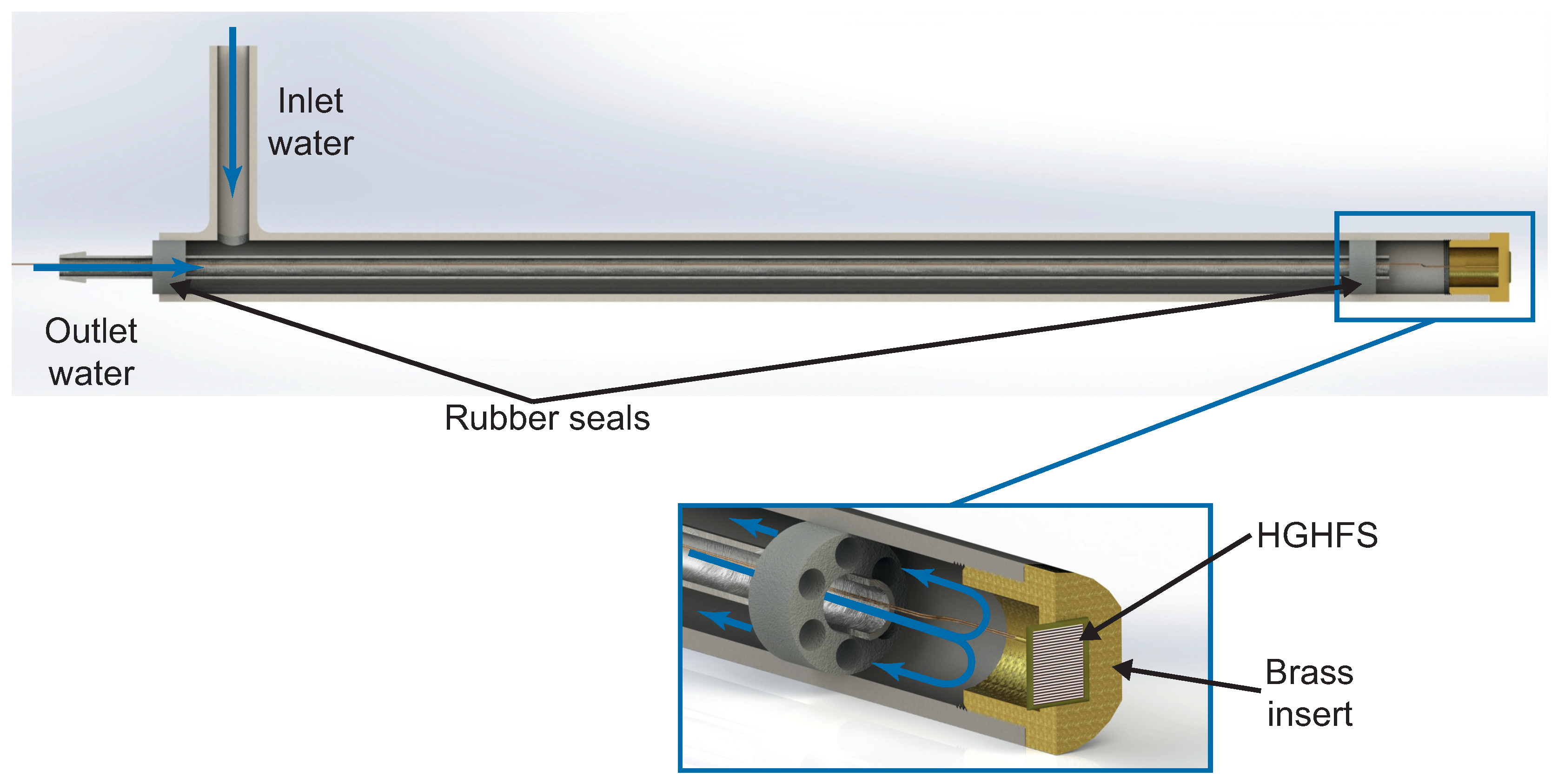
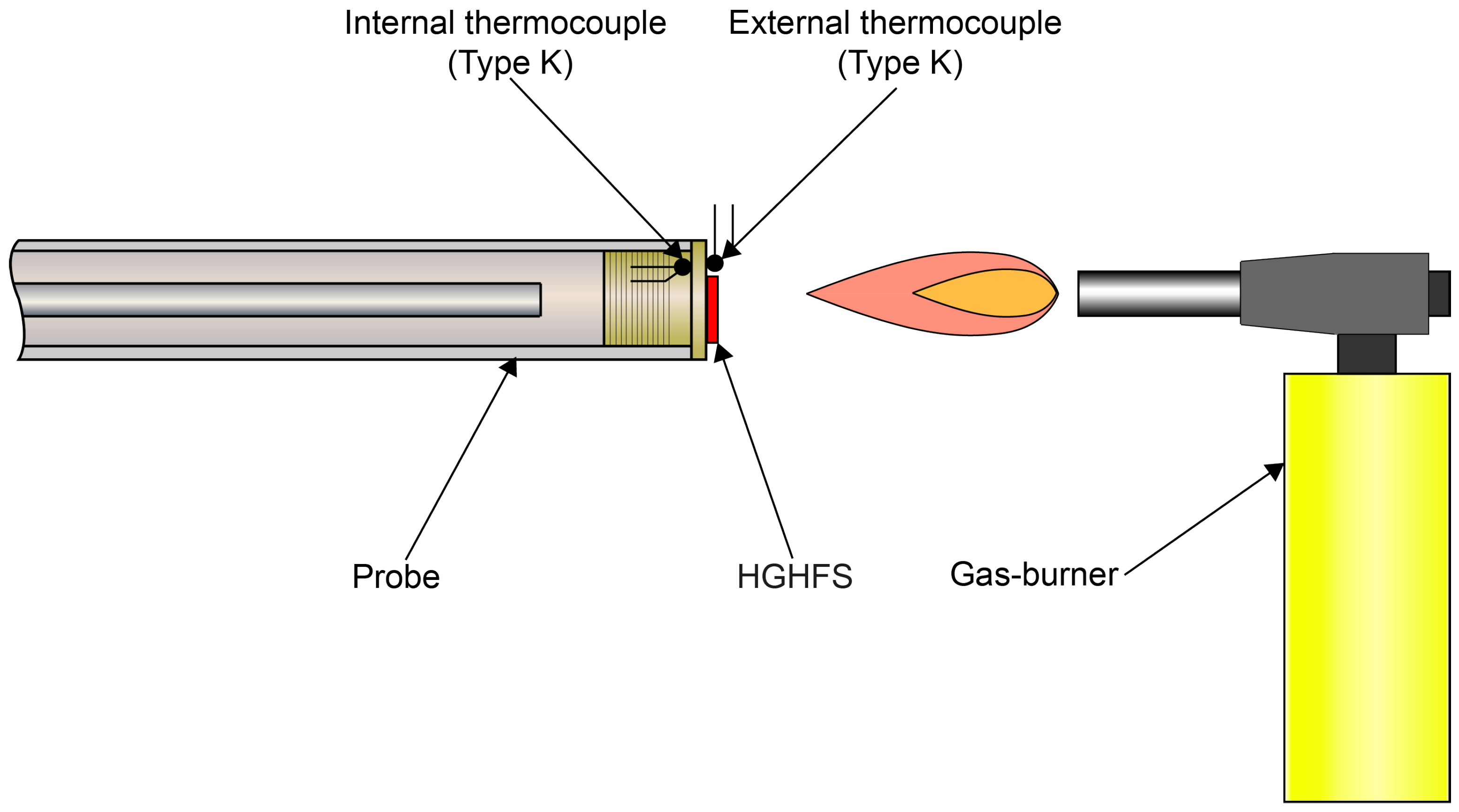
The experimental setup used here includes a measuring probe and a frame, allowing for the possibility of use with a gas or diesel burner. A probe with HGHFS for adjustment and diagnosing the burner was created. The pipe-in-pipe probe has an HGHFS mounted on a measuring insert (Figure 4). A similar design with thermocouples has been used by other researchers [3]. In our probe, temperature measurement is combined with gradient heatmetry. The temperature measurement is then used to verify the HGHFS calibration.
During the design of the probe, we considered the following main factors:
- The measuring insert dimensions must be small enough in comparison with the the flame size and large enough in comparison with the HGHFS plan-area.
- The measuring insert must be made of a material with high thermal conductivity, and the probe itself must be made of a material with low thermal conductivity.
- The dimensions of the probes and inserts should be convenient for mounting thermocouples and HGHFS, outputting wires, and supplying cooling water.
Here, the probe consists of a casing made from stainless steel, a coolant pipe, and a measuring insert (Figure 5) with high thermal conductivity made of brass.
The HGHFS is mounted on the end face of the brass insert. A K-type thermocouple is mounted near it. A similar thermocouple is installed on the opposite side of the insert. The probe enables measurement of the local heat flux when the power-generating equipment is operating. The data obtained by gradient heatmetry make it possible to investigate the operating mode in detail and adjust the fuel mass flow rate with high accuracy.
The multi-operation setup (Figure 6) allowed us to test burners of different power. In our experiments, we used two OILON burners [18].
The setup is equipped with a limiting crossbar parallel to the flame axis for probe precise positioning. The probe moves along the flame axis with a fixed pitch of 25 mm. This experiment enabled us to determine how the local heat flux from the flame is distributed along its length.
2.3. Measurement Uncertainty
Uncertainty calculations were carried out according to ISO/IEC GUIDE 98-1:2009—Uncertainty of Measurement [19], according to which uncertainty of measurement is the expression of the statistical dispersion of the values attributed to a measured quantity. The combined standard uncertainty of is calculated by the following formula:
where is the dispersion of . The values of were assumed to be known and were determined by the characteristics of the devices.
Factors contributing to uncertainty in heat flux measurements are:
- Error in the GHFS volt-watt sensitivity
- Error in measuring the GHFS area
- Errors in measurement using ADC
These errors should be evaluated as type B uncertainties, as follows:
where q is counted according to Formula (2) and the standard uncertainty of the GHFS area, that is , is equal to 2.8 × 10 m. Here, the standard uncertainty of the GHFS volt-watt sensitivity, , was assumed to be equal to 0.17 mV/W. In the experiments, a multimeter Fluke 287 was used to register the signal and was equal to 0.025% [20];
To estimate the extended uncertainty, the coverage factor was K = 2.
As a result, we obtained the relative uncertainty when measuring the heat flux as
As an example, Table 1 presents the results of the uncertainty calculation.
Analysing the contribution of the uncertainty showed that the greatest influence is conferred by the assessed accuracy of the volt-watt sensitivity . Within the framework of the proposed method, it is possible to improve the accuracy of heat flux measurement by refining the volt-watt sensitivity and using a more accurate thermo-EMF meter.
3. Experimental Results
3.1. Pilot Experiments
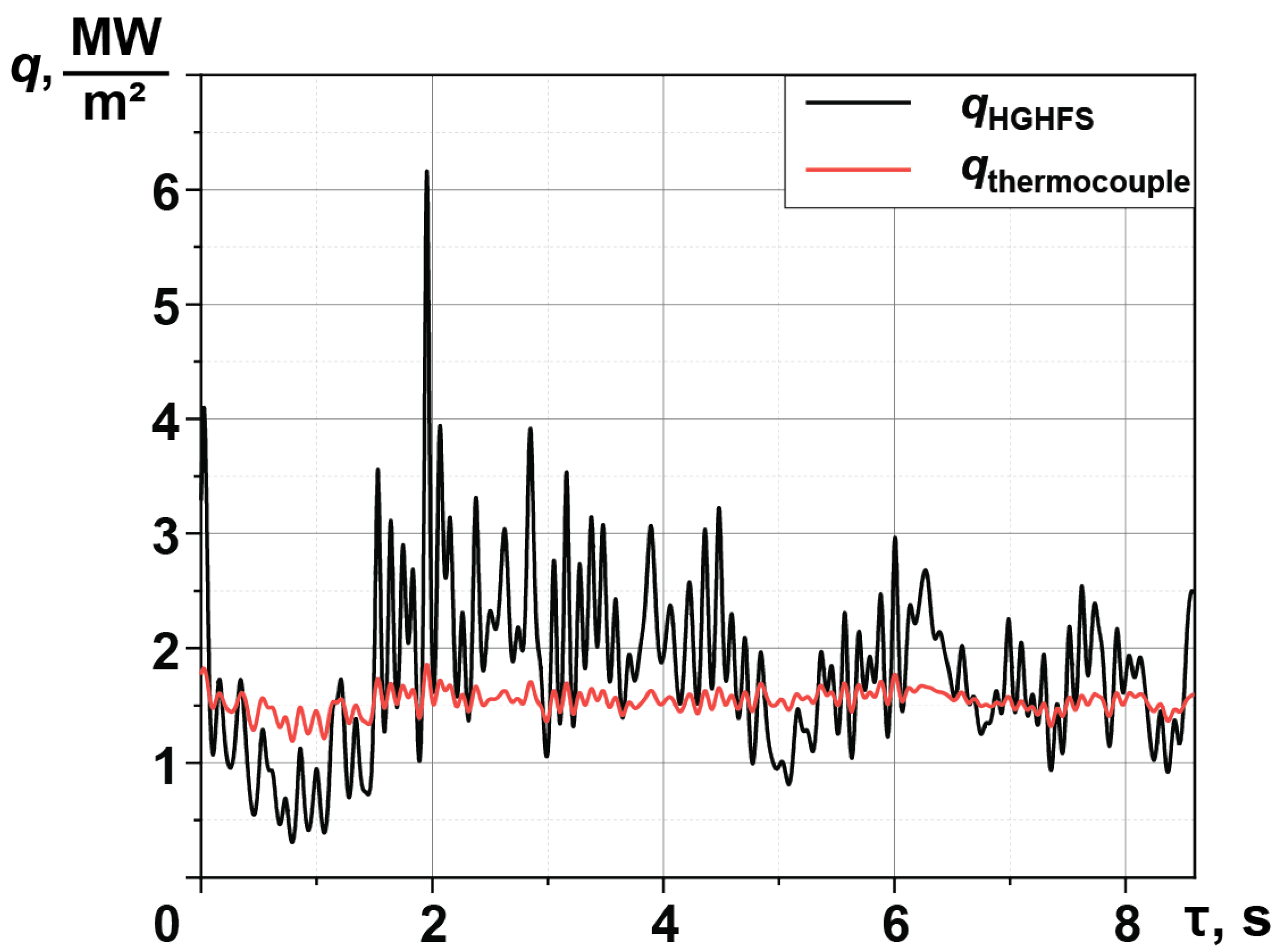
Pilot experiments were carried out using a household gas burner. The scheme of the experiments is shown in Figure 7.
The probe was mounted horizontal and blown by the flame from the burning gas. This experiment simulates the technique for obtaining a uniform temperature field, similar to an infinite plate, which simplifies the calculation of the heat flux per unit area and makes it possible to compare the results of the HGHFS and thermocouples. The data from two thermocouples and the sensor were recorded on a National Instruments analog-to-digital converter (ADC). We compared the heat flux per unit area measured by the HGHFS with the heat flux calculated from the heat transfer of the plate with known surface temperatures [21]:
where k = 110 W/(m×K) is the thermal conductivity of the metal block, and are the temperature (in K) on the external and internal surfaces of the insert, respectively, and is insert thickness (m).
The results of the comparison are shown in Figure 8.
Figure 8 demonstrates that the average heat fluxes measured by the HGHFS and calculated based on the thermocouple measurements are quite similar. Because the insert is 11 mm thick, the fluctuations in heat flux determined by the temperature measurement data are insignificant. HGHFS is not related to the thermal lag of the insert; therefore, we observe heat flux fluctuations. The disarrangement between time-averaged and does not exceed 3%.
We estimate the relative extended uncertainty of heat flux measurements about at 7%; thus, gradient heatmetry provides satisfactory results in the burning investigation.
3.2. Gas Flame
Currently, the vast majority of power plants use conventional gas as fuel. This is due to its simplicity of combustion, lack of preparatory procedures, and low level of pollutant emissions.
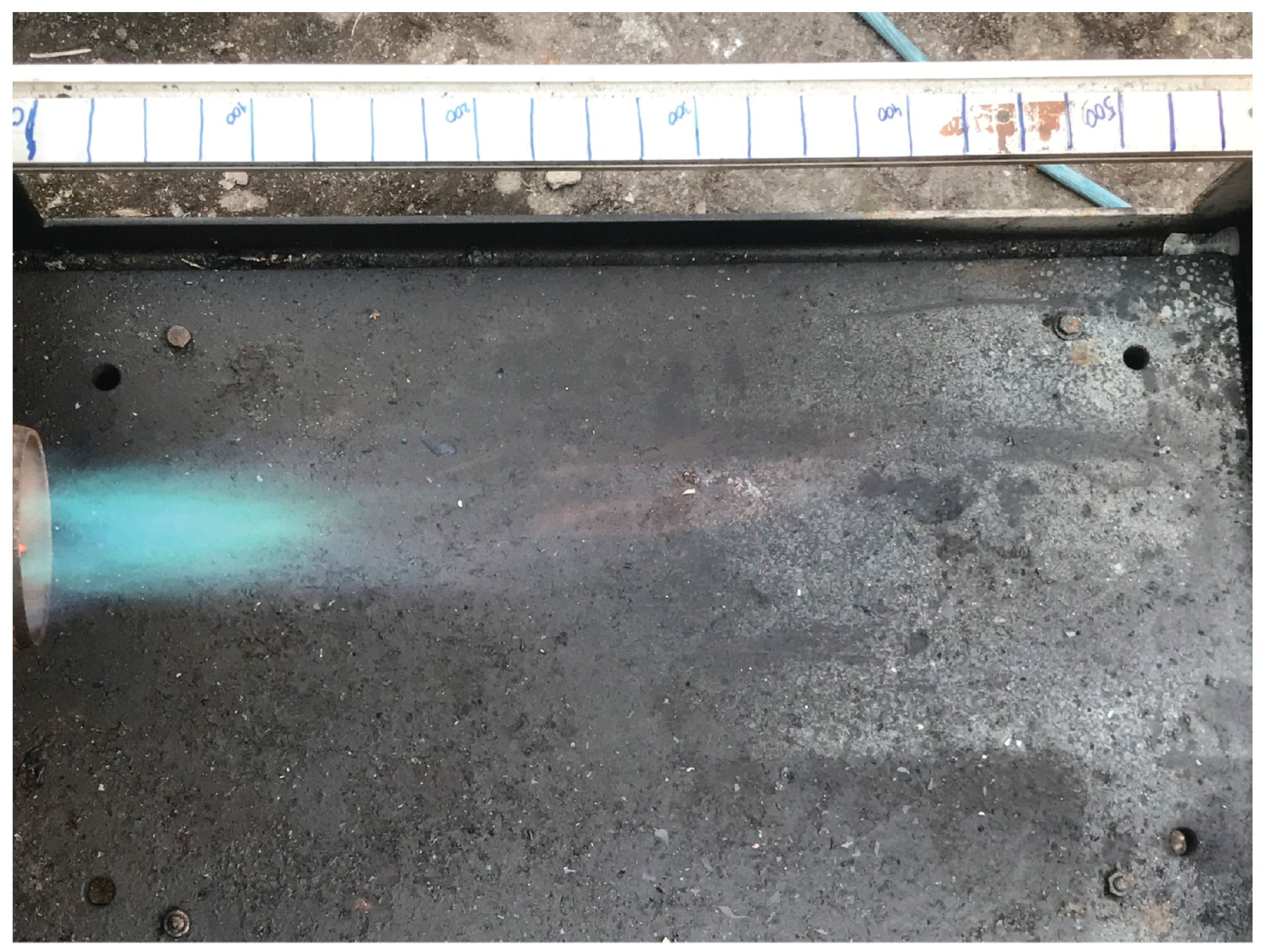
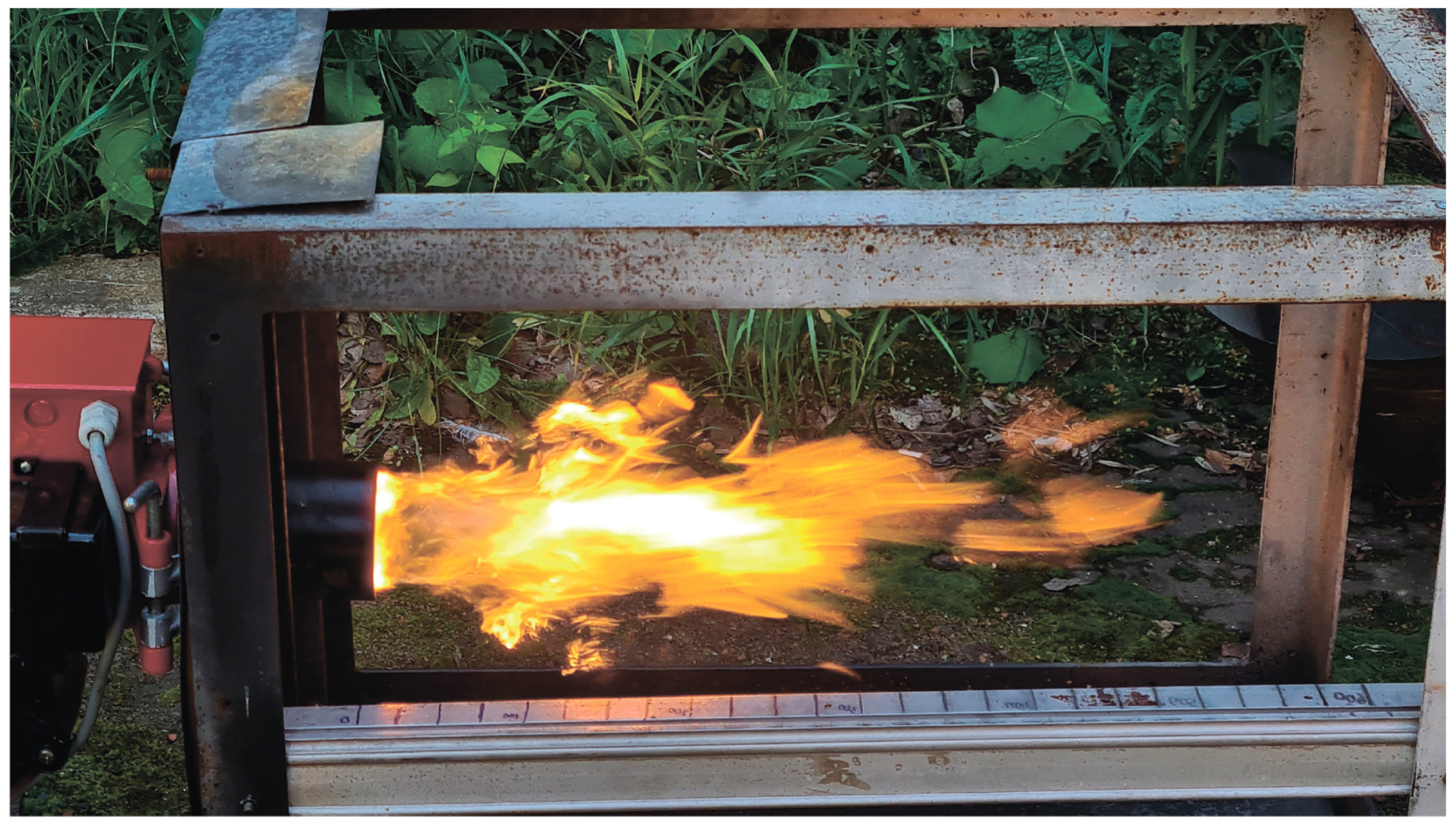
Here, we consider the heat generated by a gas flame produced by an OILON GP-6 burner [18]. The burner was mounted on the frame (Figure 6), which allowed us to investigate the heat generation along the length of the flame. Propane was used as fuel.
The combustion mode was selected in such a way as to obtain stable burning. In this operating mode, it was possible to burn gas quite efficiently (Figure 9). Propane burning with the optimal stoichiometric ratio is not accompanied by radiation in the visible spectrum.
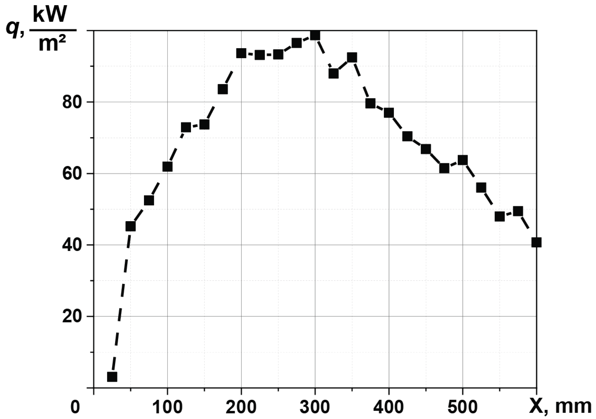
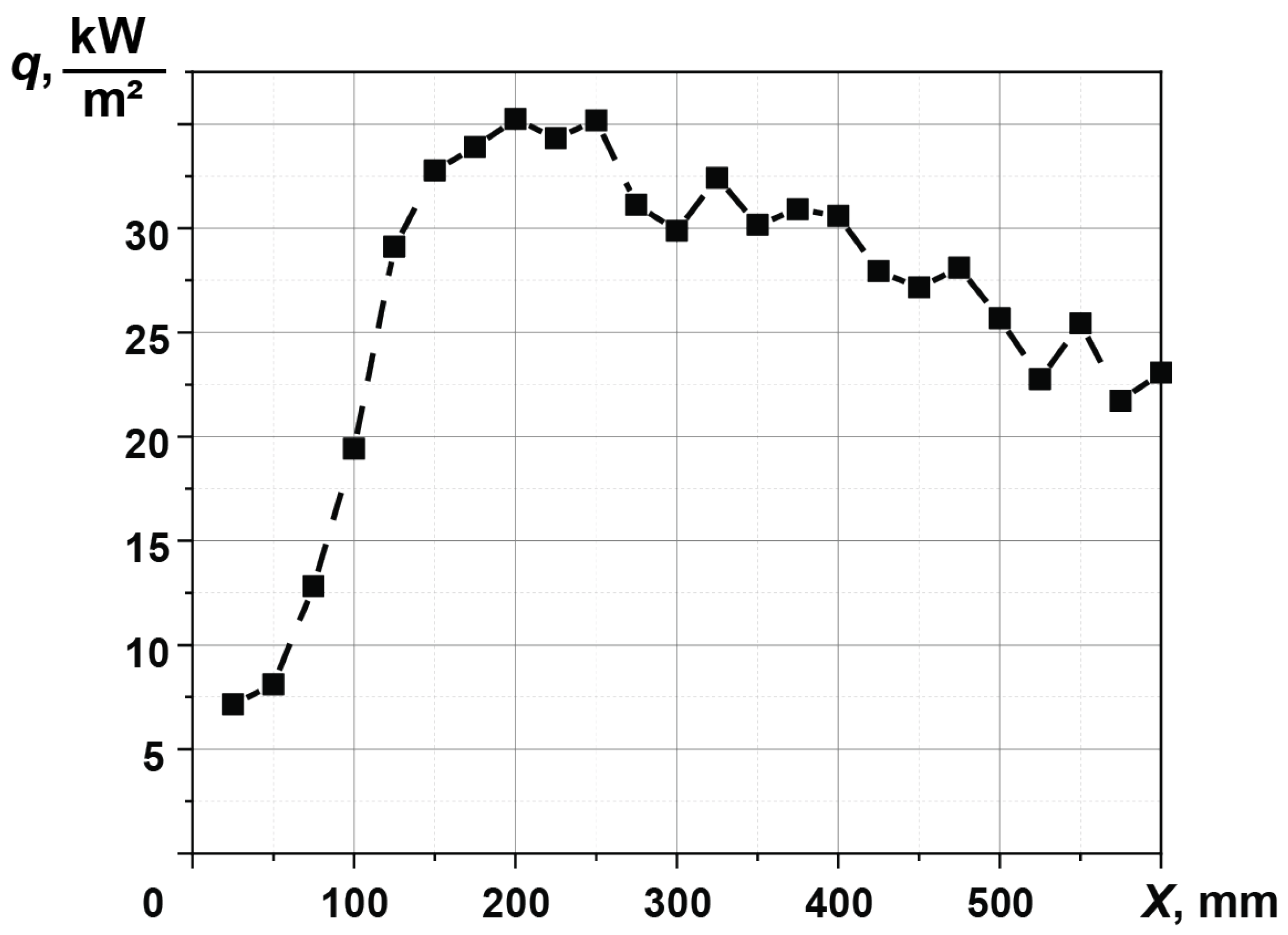
The flame turns blue as fuel and oxidant exit the burner head, which is when the gas with the largest amount of oxidant is burning. The process is then stabilized, and radiation in the visible spectrum is not observed. The results of measuring the flame heat flux are shown in Figure 10.
According to our data, three combustion zones can be distinguished. In the “cold” flame zone (x = 0…150 mm from the burner nozzle), the fuel is actively mixed with the oxidant, and small part of the fuel burns. The active combustion zone (x = 150…350 mm from the nozzle) is the area in which the optimal ratio of fuel and oxidant is maintained and maximum heat generation is observed. In the “tail” zone (x > 350 mm), the remaining fuel burns out.
The theoretical chemical reaction of propane air oxidation has the form [1]
In the our experiments, the flame temperature did not reach 2000 C; therefore, the formation of in Equation (8) can be ignored.
The heat balance equation for the reaction in (8) is
where is the actual heat generated during the combustion of gas, is the heat generated during the combustion of propane, is the heat needed to heat propane by the activation temperature, is the heat needed to heat the air to the activation temperature, is the heat carried away by the exhaust gases, and is the heat carried away by water. The calculation was performed for the temperature of t = 965 C measured by thermocouple during the experiment.
Substituting the mass flow rates calculated for the theoretical chemical reaction (8) provides = 36.6 kW. Experimental and theoretical values were compared according to the heat flux. The integral heat flux obtained in the experiment was = 71.7 kW/m, with the theoretical calculation = 73.6 kW/m. This again proves the applicability and efficiency of this methodology in the study of flame combustion.
As shown above, the average heat flux obtained in the experiment and the heat flux calculated theoretically are comparable; however, the theory does not allow for the local heat flux to be calculated. Figure 10 demonstrates the high unevenness of heat generated from the flame ( = 98.7 kW/m, = 3.1 kW/m). This suggests that it is possible to determine the zone of local overheating of the heat transfer surfaces and efficiently adjust the burner. This last conclusion opens up new perspectives on boiler design. Data on the the heat flux unsteadiness in terms of both time and surface area allows these factors to be taken into account when calculating and designing heat exchange surfaces.
3.3. Diesel Flame
The main problem with fire-tube boilers is burnout of the fire tube caused by uneven heat generation, leading to uneven scale deposition. Burnout of the fire tube can lead to a steam explosion and failure of the entire power plant.
Here, we consider the combustion of diesel fuel in an OILON KP-6 burner with a DANFOSS nozzle, a mass flow rate of 1.75 gallons, and a flame coning angle of 60 [22]. The nozzle is an important element of the burner, and can easily become clogged and fail. It is impossible to assess its operability and compliance with factory settings when the burner is in operation.
The operating mode of the burner was selected in such a way as to obtain a steady flame (Figure 11).
Burning of diesel fuel during combustion is a complex and ambiguous chemical process, and a large number of assumptions are necessary in order to calculate it [23]. When solving this problem in relation to boiler equipment, it is sufficient to consider the local heat generation and temperature field. Figure 12 shows the values of the local heat flux for a fuel mass flow rate of 7.11 kg/h.
Similar to the gas flame, three combustion zones can be distinguished: a zone of “cold” flame (x = 0…150 mm from the burner nozzle), an active combustion zone (x = 150…300 mm from the burner nozzle), and a “tail” zone (x > 300 mm) in which the flow is destabilized and the remaining fuel burns out. The tail zone features heat flux fluctuation associated with peculiarities of the flame. Because liquid fuel combustion is considered diffusive, the destabilization of the heat flux leads to the emergence of separate sources of active combustion.
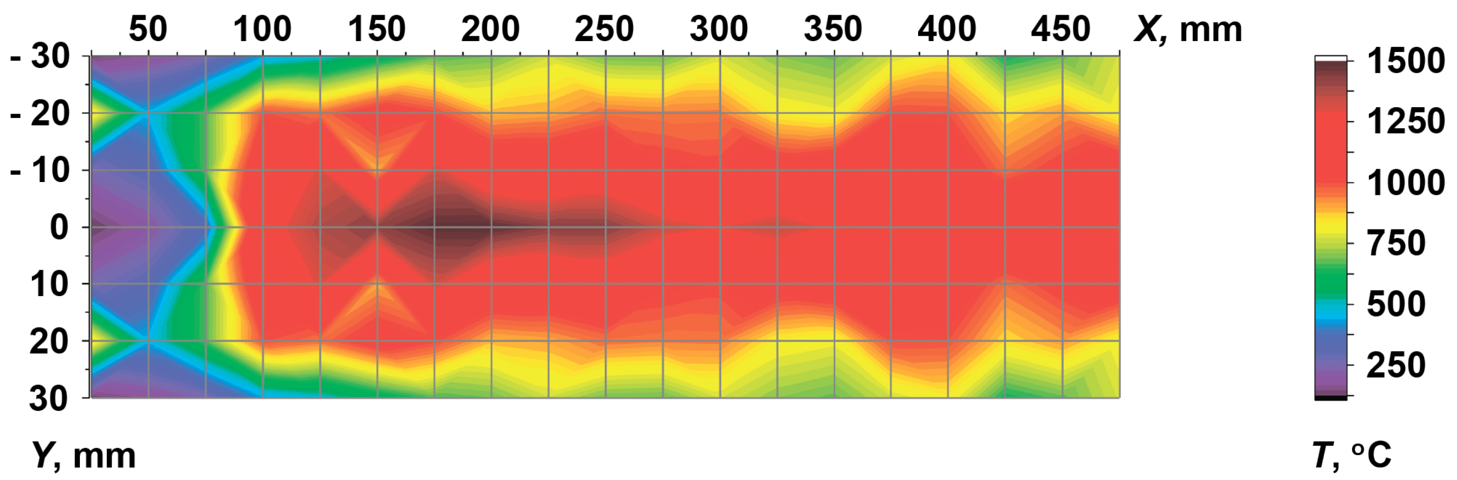
Figure 13 shows the temperature field measured in the central section of the flame. Measurements were conducted by the contact method using a K-type thermocouple. The elapsed time of the K-type thermocouple at temperatures above 1000 was experimentally determined. In our experiments, the temperature measurement time at each point was about 100 s, meaning that our results can be considered correct.
Temperature fluctuations were observed at a distance of 300 mm from the outlet section of the “burner head”, similar to the heat flux per unit area measured by the HGHFS.
The burning of a drop of liquid fuel in an oxidant is modeled as a stationary sphere, from the surface of which the fuel evaporates and reacts with the oxidant. It is impossible to calculate the flame heat generation in such a setting. When the flow is swirled, drops combine and leave the combustion area due to inertia or gravity. It is almost impossible to take this into account during calculations, and as a result it is impossible to calculate the thermal balance. If we consider a certain number of drops close to one another, we have a surface that is in direct contact with the oxidant, which results in combustion.
Here, let us make such an assumption and consider the heat transfer radiated from the flame as one from a solid body with a temperature equal to the temperature at the periphery of the flame. The flame emissivity of a liquid-fuel flame is close to 1.0; therefore, the heat flux from the flame according to the Stefan–Boltzmann law is [1]
where (W/m) is the calculated flame heat flux, (K) is average temperature of the flame periphery, and is the temperature on the surface of the probe (313 K). The calculation according to the Formula (10) provides = 31.6 kW/m, and the average integral heat flux obtained in the experiment is = 28.6 kW/m. The discrepancy of 9.5% in such an experiment can be considered acceptable.
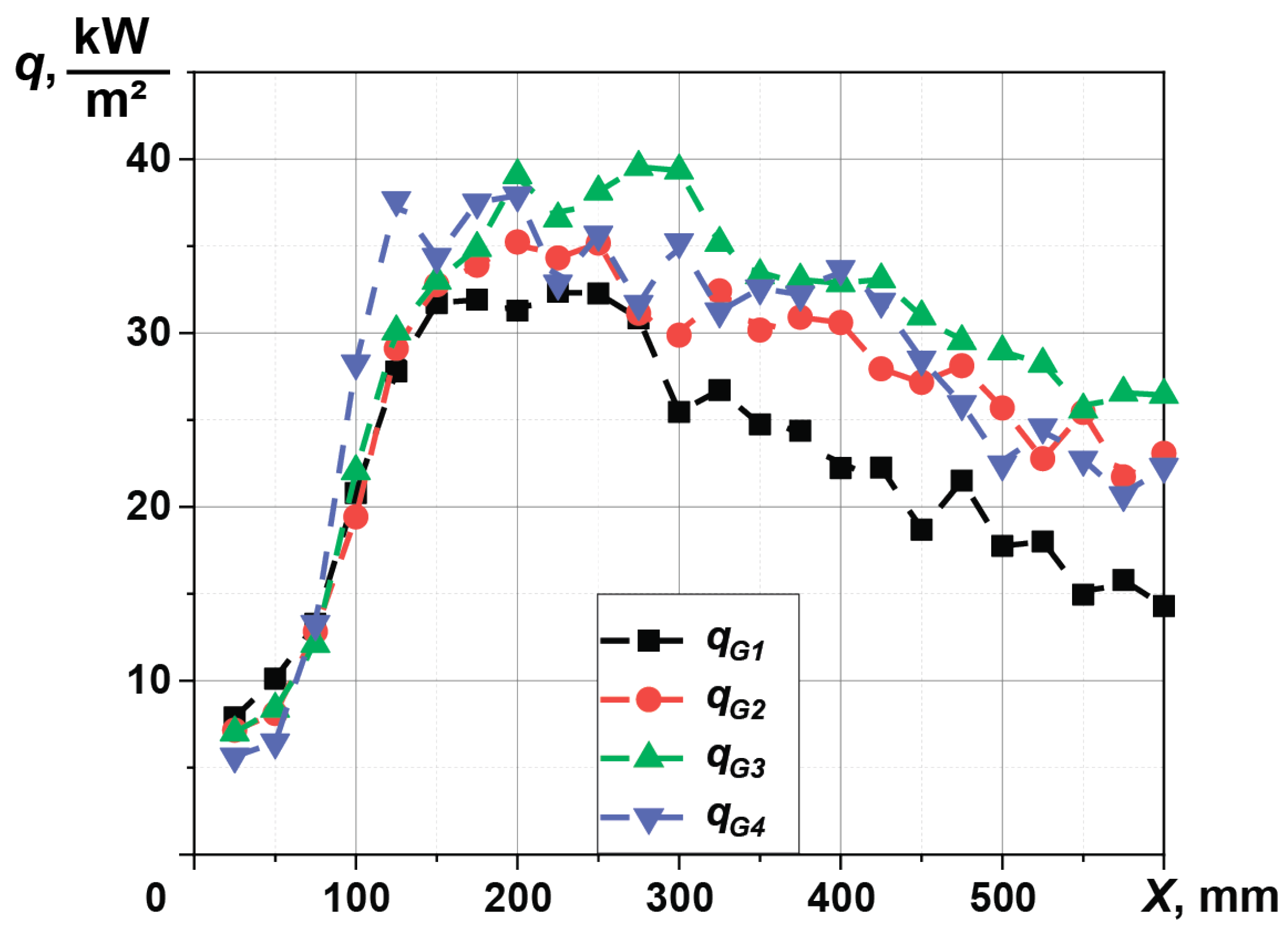
The OILON KP-6 burner is designed for a wide range of diesel mass flow rates; here, we have only considered modes with a stable flame (6.49…8.58 kg/h). The local heat flux distributions are shown in Figure 14. The curves show that the “cold” flame zone is independent of the mass flow rate. The main difference between the operating modes is the distance from the nozzle, where the local heat flux is at a maximum, as well as the fluctuation magnitude in the flame tail zone. The operating mode corresponding to the mass flow rate of 7.95 kg/h is the most stable and active.
Due to the peculiarities of the experimental setup it, is incorrect to talk about measuring the absolute pollutant emissions in the exhaust gases. It is impossible to track the air inflow from the atmosphere or the focusing of the exhaust gas flow for accurate measurement. Data on the exhaust gases are presented in relative values as relates to the maximum values. To assess the effect of fuel consumption on toxic emissions, the Testo 330i gas analyzer was used [24]. The results of the analysis are presented in Table 2.
The relative concentration of pollutant emission depending on the mass flow rate is calculated by the formula
where is the relative concentration of a substance at a specified fuel mass flow rate, is the concentration of a substance at a specified fuel mass flow rate, and is the maximum concentration of a substance.
Unfortunately, the Testo 330i gas analyzer does not allow evaluation of . In the future, we plan to use a gas analyzer that allows for measuring these parameters with high accuracy, then to analyze them in detail.
The optimal operation determined by the gradient heatmetry does not exceed the level of emissions compared to lower and higher consumption.
4. Conclusions
Despite the wide variety of probes and inserts used to determine the heat flux per unit area in the furnaces of boiler equipment, these probes are currently all based on the temperature measurement method. This approach has a number of disadvantages that mean it cannot be considered the only correct way to measure the heat flux.
Here, we have developed a unique cooled probe with HGHFS installed. The implementation of the transverse Seebeck effect with the HGHFS avoids the disadvantages described above. Therefore, it can be assumed that the gradient heatmetry is more reliable for determining the heat flux per unit area from the burner flame.
A pilot experiment in which the heat flux was compared using both temperature measurements (as most authors do) and gradient heatmetry showed the adequacy and applicability of the proposed method. At the same time, unlike thermocouples, HGHFS has a fast response time, making it possible to measure the slightest fluctuations during operation of the burners.
Comparison of the experimental values of the heat flux from the flame with the calculated values showed the reliability of our results. The discrepancy between the experimental and calculated values did not exceed 10%.
Based on the obtained temperature fields and distribution of the heat flux per unit area, it was possible to determine three main combustion zones realized during flaring of any fuel. Based on the gradient heatmetry data and gas analysis of the concentration of flue gases, it was possible to select and justify the choice of the most efficient mode of operation of the OILON KP-6 diesel burner.
This approach allows a reliable method for controlling heat generation in the furnace of any boiler equipment to be organized, permitting greater fine-tuning of industrial burners and the determination of their optimal operating mode.
Author Contributions
Conceptualization, V.M.P. and Y.V.A.; methodology, P.G.B. and A.V.P.; validation, V.M.P. and Y.V.A.; formal analysis, S.Z.S. and V.Y.M.; investigation, P.G.B. and A.V.P.; resources, V.M.P.; writing—original draft preparation, P.G.B.; writing—review and editing, S.Z.S. and V.Y.M.; visualization, P.G.B. and A.V.P.; supervision, V.Y.M.; project administration, S.Z.S. All authors have read and agreed to the published version of the manuscript.
Funding
This research received no external funding.
Data Availability Statement
Not applicable.
Conflicts of Interest
The authors declare no conflict of interest.
Abbreviations
The following abbreviations are used in this manuscript:
| LHV | Lower Heating Value |
| GHFS | Gradient Heat Flux Sensor |
| ATE | Anisotropic Thermoelemnt |
| HGHFS | Heterogeneous Gradient Heat Flux Sensor |
| ADC | Analog to Digital Converter |
References
- Glassman, I.; Yetter, R.A.; Glumac, N.G. Combustion, 5th ed.; Elsevier: Amsterdam, The Netherlands, 2014; 757p. [Google Scholar]
- Kemelman, D.N.; Eskin, N.B.; Davidov, A.A. Adjustment of Boiler Installations: Handbook; Energiya Publ.: Moscow, Russia, 1976; p. 344. [Google Scholar]
- Zhang, D.; Shi, H.; Meng, C.; Wu, Y.; Zhang, H.; Zhou, W.; Ran, S. Measurements on Heat Flux Distribution in a Supercritical Arch-Fired Boiler. In Clean Coal Technology and Sustainable Development; Yue, G., Li, S., Eds.; Springer: Singapore, 2016; pp. 207–212. [Google Scholar]
- Martucci, A.; De Gregorio, F.; Musto, M.; Petrella, O.; Marciano, L.; Rotondo, G.; Gaudino, E. Innovative calibration methodology for gardon gauge heat flux meter. In Proceedings of the IEEE 7th International Workshop on Metrology for AeroSpace (MetroAeroSpace), Pisa, Italy, 22–24 June 2020; pp. 288–293. [Google Scholar]
- Pullins, C.A.; Diller, T.E. Direct Measurement of Hot-Wall Heat Flux. J. Thermophys. Heat Transf. 2012, 26, 430–438. [Google Scholar] [CrossRef]
- Guillot, E.; Alxneit, I.; Ballestrin, J.; Sans, J.L.; Willsh, C. Comparison of 3 heat flux gauges and a water calorimeter for concentrated solar irradiance measurement. Energy Procedia 2014, 49, 2090–2099. [Google Scholar] [CrossRef] [Green Version]
- Northover, E.W.; Hitchcock, J.A. A heat flux meter for use in boiler furnaces. J. Sci. Instrum. 1967, 44, 371–374. [Google Scholar] [CrossRef]
- Arai, N.; Matsunami, A.; Churchill, S.W. A review of Measurements of Heat Flux Density Applicable to the Field of Combustion Experimental. Therm. Fluid Sci. 1996, 12, 452–460. [Google Scholar] [CrossRef]
- Schulte, E.H.; Kohl, R.F. A review of measurements of heat flux density applicable to the field of combustion. Exp. Therm. Fluid Sci. 1969, 40, 1420–1427. [Google Scholar]
- Hager, N.E., Jr. Thin Foil Heat Meter. Rev. Sci. Instrum. 1965, 36, 1564–1570. [Google Scholar] [CrossRef]
- Klems, J.H.; DiBartolomeo, D. Large-area, high-sensitivity heat-flow sensor. Rev. Sci. Instrum. 1982, 53, 1609–1612. [Google Scholar] [CrossRef] [Green Version]
- Mityakov, A.V.; Mityakov, V.Y.; Sapozhnikov, S.Z.; Chumakov, Y.S. Measurement of Instantaneous Values of a Heat Flux on a Vertical Heated Surface under Conditions of Free-Convection Heat Transfer. High Temp. 2002, 40, 620–625. [Google Scholar] [CrossRef]
- Sapozhnikov, S.Z.; Mityakov, V.Y.; Mityakov, A.V. Bismuth-Based Gradient Heat-Flux Sensors in Thermal Experiment. High Temp. 2004, 42, 629–638. [Google Scholar] [CrossRef]
- Sapozhnikov, S.; Mityakov, V.; Mityakov, A. Heatmetry: The Science and Practice of Heat Flux Measurement; Springer International Publishing: Berlin/Heidelberg, Germany, 2020. [Google Scholar]
- Sapozhnikov, S.Z.; Mityakov, V.Y.; Seroshtanov, V.V.; Gusakov, A.A. The Combination of PIV and Heat Flux Measurement in Study of Flow and Heat Transfer Near a Circular Finned Cylinder. In Proceedings of the International Conference on Optical Methods of Flow Investigation, Moscow, Russia, 24–28 June 2019; Volume 1412. [Google Scholar]
- Mityakov, V.Y.; Sapozhnikov, S.Z.; Zainullina, E.R.; Babich, A.Y.; Milto, O.A.; Kalmykov, K.S. Gradient Heat Flux Measurement while Researching of Saturated Water Steam Condensation. In Proceedings of the International Conference “Problems of Thermal Physics and Power Engineering” (PTPPE-2017), Moscow, Russia, 9–11 October 2017; Volume 891. [Google Scholar]
- Sapoznikov, S.Z.; Mityakov, V.Y.; Gusakov, A.A.; Pavlov, A.V.; Bobylev, P.G. Gradient Heatmetry for Boiling of Underheated Water on Spherical Surface. J. Phys. Conf. Ser. 2020, 1683, 1683. [Google Scholar] [CrossRef]
- Available online: https://oilon.spb.ru/ (accessed on 11 November 2022).
- ISO/IEC Guide 98-1:2009–Uncertainty of Measurement—Part 1: Introduction to the Expression of Uncertainty in Measurement. Available online: www.iso.org/standard/ (accessed on 12 November 2022).
- Available online: https://flukeshop.ru/multimetr-fluke-287/ (accessed on 30 November 2022).
- Benjamin, G. Heat Transfer; McGraw-Hill: New York, NY, USA, 1961; p. 454. [Google Scholar]
- Available online: https://www.danfoss.com/ (accessed on 11 November 2022).
- Lakshminarayanan, P.A.; Aghav, Y.V. Modelling Diesel Combustion; Springer: Berlin/Heidelberg, Germany, 2010. [Google Scholar]
- Available online: https://www.testo.ru/ (accessed on 13 November 2022).
Figure 1.
Sketch of Gardon heat flux gauge for convective heat transfer measurements [4].
Figure 1.
Sketch of Gardon heat flux gauge for convective heat transfer measurements [4].

Figure 2.
GHFS scheme (a) and general view (b) [14]: 1—anisotropic thermopower element (ATE); 2—mica; 3—bismuth soldering; 4—current leads; 5—lavsan base.
Figure 2.
GHFS scheme (a) and general view (b) [14]: 1—anisotropic thermopower element (ATE); 2—mica; 3—bismuth soldering; 4—current leads; 5—lavsan base.

Figure 3.
HGHFS scheme (a) and general view (b).

Figure 4.
Experimental probe scheme.

Figure 5.
Measurement insert design.

Figure 6.
Experimental setup for measuring the heat flux during combustion: 1—metal frame; 2—burner; 3—crossbar with divisions.
Figure 6.
Experimental setup for measuring the heat flux during combustion: 1—metal frame; 2—burner; 3—crossbar with divisions.

Figure 7.
Pilot study scheme.

Figure 8.
Heat flux graph for pilot studies.

Figure 9.
Propane combustion in OILON burner.

Figure 10.
Local heat flux along the gas flame.

Figure 11.
Diesel fuel combustion in OILON burner.

Figure 12.
Local heat flux along the diesel flare.

Figure 13.
Temperature field in the cross-section of the diesel flame.

Figure 14.
Dependence of the local heat flux on the longitudinal coordinate at various fuel mass flow rates: = 6.5 kg/h, = 7.1 kg/h, = 7.95 kg/h, = 8.6 kg/h.
Figure 14.
Dependence of the local heat flux on the longitudinal coordinate at various fuel mass flow rates: = 6.5 kg/h, = 7.1 kg/h, = 7.95 kg/h, = 8.6 kg/h.


Table 1.
The uncertainty budget for heat flux measurement (diesel flame; diesel mass flow rate = 7.95 kg/h; x = 125 mm).
Table 1.
The uncertainty budget for heat flux measurement (diesel flame; diesel mass flow rate = 7.95 kg/h; x = 125 mm).
| Quantity | Value | Standart Uncertainty | Probability Distribution | Sensitivity Coefficient | Uncertainty Contribution |
|---|---|---|---|---|---|
| , mV/W | 4.97 | 0.17 | B | −7238 | 1230.5 |
| A, m | 25 × 10 | 2.8 × 10 | B | −144.2 × 10 | 40.32 |
| E, mV | 4.488 | 0.025 | B | 16.1 × 10 | 401.6 |
| q, W/m | 36.05 × 10 | 1295.0 | B | ||
| , % | 7.18 |
Table 2.
Relative pollutant emission concetration depending on the diesel mass flow rate.
| Flow-Rate, kg/h | CO | nCO | O |
|---|---|---|---|
| 7.11 | 0.80 | 1.00 | 0.92 |
| 7.95 | 0.62 | 0.22 | 1.00 |
| 8.58 | 1.00 | 0.07 | 0.84 |
Publisher’s Note: MDPI stays neutral with regard to jurisdictional claims in published maps and institutional affiliations. |
© 2022 by the authors. Licensee MDPI, Basel, Switzerland. This article is an open access article distributed under the terms and conditions of the Creative Commons Attribution (CC BY) license (https://creativecommons.org/licenses/by/4.0/).
Share and Cite
MDPI and ACS Style
Bobylev, P.G.; Pavlov, A.V.; Proskurin, V.M.; Andreyev, Y.V.; Mityakov, V.Y.; Sapozhnikov, S.Z. Gradient Heatmetry in a Burners Adjustment. Inventions 2022, 7, 122. https://doi.org/10.3390/inventions7040122
AMA Style
Bobylev PG, Pavlov AV, Proskurin VM, Andreyev YV, Mityakov VY, Sapozhnikov SZ. Gradient Heatmetry in a Burners Adjustment. Inventions. 2022; 7(4):122. https://doi.org/10.3390/inventions7040122
Chicago/Turabian StyleBobylev, Pavel G., Andrey V. Pavlov, Vyacheslav M. Proskurin, Yuriy V. Andreyev, Vladimir Yu. Mityakov, and Sergey Z. Sapozhnikov. 2022. "Gradient Heatmetry in a Burners Adjustment" Inventions 7, no. 4: 122. https://doi.org/10.3390/inventions7040122