1. Introduction
One of the emerging topics related to modern radar systems designed for probing closed spaces such as rooms through the wall or other dense obstacles is detecting the presence of people, estimating their coordinates, and further possible reconstruction of the trajectories describing their movement. On one hand, according to their basic application scenario, through-the-wall radars can be called a subclass of short-range radars [
1]. On the other hand, a typical through-the-wall radar (TWR) differs from the majority of short-range radars designed to operate in open spaces in at least two ways [
2,
3]. The first is the large attenuation of the signals caused by radio waves propagating through the wall which, as a material, has a much greater absorption rate than air. The second is the inevitable presence of a significant number of interfering clutters caused by re-reflections of the signals of interest (SOI) from stationary objects displaced all over the room, such as pieces of furniture, walls, floor, ceilings, wires, etc.
The detection of moving people is demanded in many practical scenarios, ranging from enhanced monitoring systems [
4] and security systems [
5] to specialized solutions providing assistance to people with disabilities [
6,
7]. The reliable identification of humans, who remain still for a long time because of injury, becomes crucial when it comes to making the decision of starting fast rescue operations, e.g., after earthquakes [
8] or other life-threatening disasters [
9], where people fixed in different poses can be blocked in cavities made of fallen bricks or damaged concrete panels. In a radar signal-processing view, a rough yet realizable delimiter between the cases of moving and non-moving humans can be drawn relying upon whether the human stays in the same range of resolution cells at two consecutive radar measurements or not. The latter case is better developed in radar signal processing in general since it requires the methods of moving target indication (MTI) which are basically resembling those that are used in other types of radar systems [
10].
In contrast, the basic principles laying behind the detections of non-moving humans consist in the identification of features known as the vital signs [
11]. The reason why the vital sign can be detected by a radar system is the relatively small displacements of reflecting surfaces caused by the processes in a live human body. Three main vital signs are respiration, heartbeat, and body movements. The respiration expresses in quasi-periodic change in the volume of the chest [
12], leading to rhythmic displacement of the chest wall by 0.5 to 2 cm forward and backward. The heartbeat is a more regular process in the short term; it includes regular changes in the volumes of ventricles and atria of the heart [
13] and subsequent pulse waves mostly affecting the main arteries, resulting in a total displacement measured as 0.1 to 0.5 cm. The class of vital signs generally described as the body movement is rather wide since it includes the variety of muscle-driven motions ranging from deliberate ones, such as gestures [
14], to natural tremors [
15,
16], characterized mostly as realization of a non-stationary random process [
17,
18]. In the signal-processing view, signals reflected from a non-moving human tend to cause interframe oscillations in the amplitude and phase of the value measured in the resolution cells where the target is continuously observed. Therefore, such a target can be called oscillating.
The signals reflected from people in TWR can be highlighted by using methods of selecting signals related to the group of techniques referring to the basic idea of processing signals generated by moving or oscillating targets. They are briefly described below. The first group represents inter-period subtraction (IPS), thoroughly described in [
19] in relation to general radar signal processing. The second group is formed by the local non-parametric estimators, especially those aimed at local sample variance [
20,
21]. The different modifications of the Fourier transform method [
22,
23] constitute the third group, which is expected to be valuable for slow time counts. The methods belonging to the groups described above have the greatest computational applicability due to the simplicity of the underlying computing. In addition, the results obtained by them are usually rather easy to interpret, which allows an experienced researcher to make a slight modification in order to tune the methods better to a particular problem being solved.
However, over recent decades researchers have been extensively working on new techniques which are expected to provide better performance at the cost of more complicated models and mathematical transformations. Thus, methods based on Hilbert-Huang transform [
24,
25] and wavelet transforms [
26,
27,
28] show clear examples going beyond the limitations of standard Fourier transform. Other known methods showing promising performance are based on the independent component analysis (ICA) [
29], variational mode decomposition (VMD) [
30] and sparse sensing [
31].
An alternative approach for detection can be established via implementation of the algorithms based on artificial neural networks (ANN) in radar-processing units. Such algorithms as shown in [
32,
33] may potentially provide a higher level of overall performance. However, they require a training step to be properly conducted. If the training is carried out on model data only, the detection in real-life can deteriorate due to the complex environment of the room being probed by the radar.
Regardless of a processing method, in most cases the signal of interest (SOI) appears to be rather weak since it remains hidden in the background noise or more intensive reflectors, especially when probing is performed through thick brick or concrete walls, or the distance to the target is relatively large compared to the distances to other reflectors. The general condition taking place at the detection can be described in terms of signal-to-noise ratio (SNR), whose value turns out to be rather small. Thus, in a common scenario described above, it rarely exceeds units of dB, which may be insufficient for reliable detection of the targets if this detection is based on simple or immediate methods. In other types of radar applications, the increase in SNR can be achieved by enlarging the power of the SOI, leading simply to gaining the emitted waveform. However, it can hardly be a way in the current case since the power of radiated signals is strictly limited by the levels where it remains safe for those applications which involve human beings. Under these restrictions, an increase in the energy of the probing signal can be achieved by increasing its duration. One of the promising ways of achieving this has led to exploiting stepped frequency continuous wave (SFCW) signals in radars [
34] instead of more traditional ultra-wideband video pulse signals [
35], or Doppler radars [
36].
The increasing interest shown by researchers in utilizing SFCW signals is determined by their properties [
37]. Roughly speaking, SFCW exhibits a great flexibility, consisting in simultaneously choosing a time duration long enough to accumulate the energy and achieve a frequency bandwidth large enough for the desired size of the range resolution cell [
38,
39]. SFCW signals have become a more realizable choice in modern TWR systems over the last two decades of processing methods [
40,
41,
42]. However, the well-known advantages of SFCW signals, such as providing high energy and high resolution up to units of centimeters [
43,
44], cause some difficulties concerning their accurate generation and further processing [
45]. One of their sources is a non-uniform curve of the amplitude-frequency characteristics caused by the transmitting and receiving paths the signals go through in the hardware part of the radar system. Nevertheless, these difficulties can be overcome by means of techniques involving hardware and software refinement applied to the radar systems. They usually propose introducing calibration coefficients, weighting functions of frequency samples or frequency filters of interference rejection which can be obtained by measurements in echoless chambers [
46,
47].
This paper presents a specially designed method which is aimed at improving the performance of signal processing in TWR utilizing SFCW probing signals. Combining two classical techniques—interperiod subtraction and local sample variance estimators, the method was developed so that it remains effective for detecting the reflections from both moving and non-moving (stationary) people.
The rest of the paper is organized as follows.
Section 2 describes the radar site and main parameters of the signals exploited by the radar system, which also characterizes the width of its range resolution cell and provides the waveform of its point target response function. The main algorithm used for identifying stationary and moving targets in radar images are presented in
Section 3. The list includes two well-known algorithms: interperiod subtraction and local variance, and a new one developed by the authors as a normalized difference sample method.
Section 4 presents the results of computer simulation which reveals the benefits of the proposed method as long as it is applied to signals interfered by additive noise while SNR is moderate. The results of the field experiments conducted with the working SFCW radar prototype is given in
Section 5 where the advantage of the proposed method is proven by real data. The brief comments on the obtained results are given at the end of
Section 4 and
Section 5 regarding the numerical and field experiments. The discussion over results and the comparison between proposed radar system and other systems exploiting SFCW signals are given in
Section 6. The paper ends with conclusion summarizing the theoretical and practical results.
2. Characteristics of Site, Radar, Targets and Sensing Conditions
2.1. Radar Measurement Site Description
The map of the site for radar measurements is shown in
Figure 1. Basically, the radar testing site is a specially prepared room whose length is larger than its width. All radar equipment, the dense wall, and humans involved in the test are placed within the room.
The radar control and processing site (RCPS) consists of a radar system prototype and a personal computer integrated by a specialized extension board. The personal computer is a high-performance working station running a Linux-based operating system. The control panel of the radar system is implemented as an application with a Windows-based graphic user interface where the main parameters are to be set and the data acquisition process can be initiated. The antenna system (AS) is an essential part of the radar hardware and is used both for emitting and receiving electromagnetic waves.
There was a forward wall (FW) made of a dense material such as brick or concrete. The width of the FW is denoted as d. Typically FW was installed at distance RFW from the AS. This distance is assumed to be short and typically 5–20 cm. FW was actually a big block equipped with a wheeled rack at the bottom in order to make it easy to change where it was put up or to remove it completely.
The removable back wall (RBW) was placed at distance L. This wall could be easily removed to let the propagating electromagnetic wave leave the room for an open space. This prevented the site from back reflection essential for conducting research experiments as well as making some calibration steps between standard cycles of measurements.
The human beings in the test could move freely between forward and back walls as well as stand still, sit on a wooden chair, or lie on a wooden bench or directly on the room floor. The RCPS is equipped with an emergency switch intended to shut down the system in case of sudden instability of the output-emitting power, which could potentially exceed the safety level.
The range axis denoted by
r in
Figure 1 was directed by the normal vector of propagating an electromagnetic wave emitted by the radar. It was aligned to the length of the room and its origin was chosen close to the phase center of the AS.
2.2. Characteristics of Radar
Let us consider a radar system continuously monitoring the room or some hollow space through the wall. The periodic probing performed by the system is carried out by emitting the SFCW signal whose repetition period is denoted by Tr. The parameters of the signal used will define the main characteristics of the radar system. Their list is the following:
f0 is the carrier frequency of the first pulse (the initial frequency);
Δf—the frequency change step;
N—the number of pulses;
Ts—the duration of one frame.
These parameters allow one to express two principal characteristics of the radar system, namely the maximum unambiguous range
Rmax and the range resolution Δ
R by the following ratios [
34,
43]:
where
c denotes the propagation speed of radio waves. In addition, it is important to notice that product
is the effective frequency bandwidth occupied by the SFCW signal.
During the time interval
between sequential probes, the reflected signals are being received, converted to samples of digital data, recorded to RAM memory and primary processed in the radar system. The complex-valued samples of
k-th period formed in the radar analog-to-digital converter (ADC) receiving the analog waveforms at the output of the quadrature phase detector are denoted by
, where the discrete-time is marked with time instants
,
, and their sampling step is equal to the duration of one pulse of the SFCW signal. The whole sequence of these samples constituting the
k-th probing period forms a column vector
where
K is the total number of observation periods. Two-dimensional matrix
characterizes all the data received by the radar system over the observation time
KTr.
Further processing of the samples of the SFCW signal in order to restore the profile in the
k-th sensing period was carried out by means of applying the inverse discrete Fourier transform (IDFT) to each column of the matrix
S. In order to increase the duration of the scanning and use the fast Fourier transform (FFT) instead of DFT, each column of the matrix
S was padded with tail zeros to the total number
[
22]. This leads to the matrix stacked by columns:
where
,
denotes
N-point DFT, performed on its vector argument
X. The absolute values
of the vector components
characterize the reflective properties of the objects located over the ranges for the
k-th probing period
The vectors
S(k) and
G(k) (
k = 1,…, K) are also called frames, and the integers
n and
k respectively denote the indices of the ‘fast’ and ’slow’ time [
10,
23].
In the case where a point target is in a certain period with the number
k, a target response function (TRF) is formed in the space of the samples of vector
G(k), whose envelope, provided there is no noise, exhibits the waveform of a certain function visually resembling the envelope of the absolute values of the spectrum of a rectangular radio pulse defined by its samples in discrete time domain [
22].
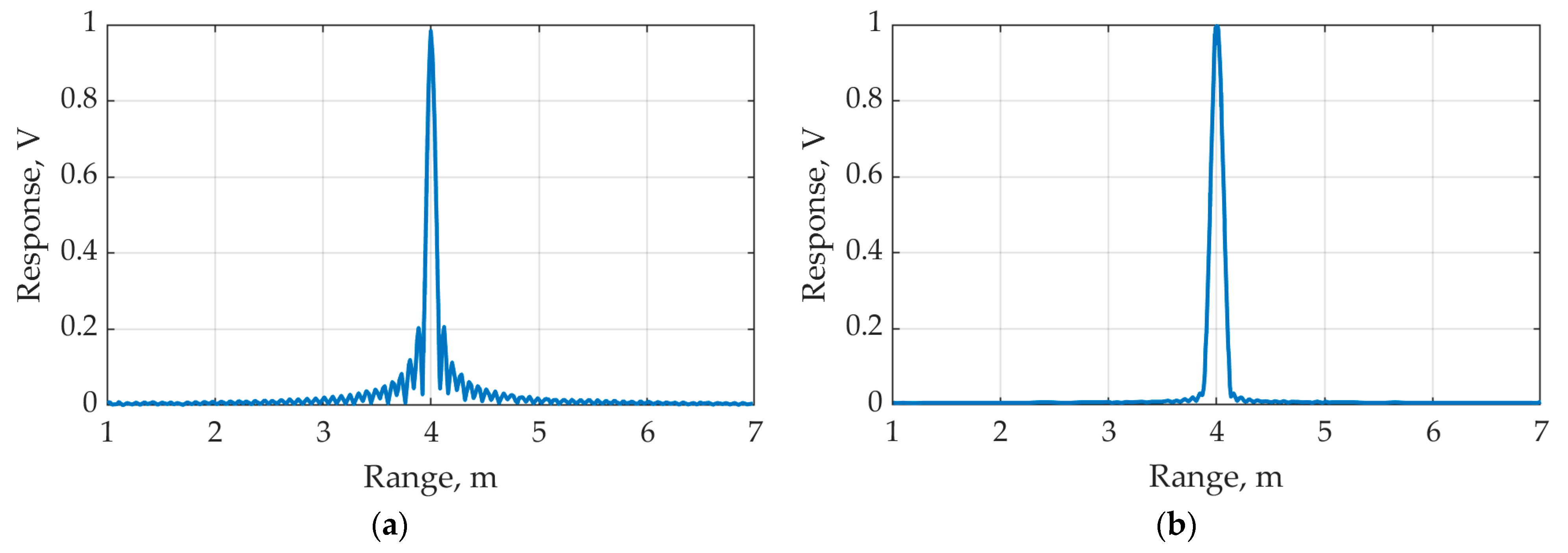
A typical view of a point TRF normalized by the maximum value in the absence of any interference or noise is shown in
Figure 2. The curve corresponds to the SFCW signal with parameters
f0 = 1 GHz, Δ
f = 5 MHz,
N = 375, where the distance to the reflecting target was 5 m. The forming of the range profile using reverse FFT operations required
Np = 2048 points, so the values of discrete samples in the figure were represented as a continuous interpolating line for the sake of easing visual perception.
The chosen values of the SFCW signal parameters provided a resolution of 0.08 m in range (see (1)), which was in accordance with
Figure 2a where a rectangular window for processing the SFCW signal was used when constructing the TRF whose width was typically estimated at the level of 0.7.
Decreasing the sidelobe level was achieved by means of weighting windows technique [
48]. Thus, the Kaiser window [
49] with parameter 4 was expertly chosen. The TRF depicted in
Figure 2b corresponded to the same SFCW signal when multiplying vectors
S(k) on the window function.
Multiplicative weighting with the window functions made it possible to reduce the level of the side lobes of the TRF, however, it led to a deterioration in the range resolution as a result of the expansion of the main lobe of the TRF [
23]. The chosen window increased the resolution in about 1.25 times, which was considered acceptable. If the local peak did not fit the time instant, its position could be refined with curve interpolation techniques, e.g., fast polynomial algorithm [
50,
51].
The matrix
S (or
G) consisted of samples describing the results of probing in one corner sector, which could cover the entire controlled space of the observed room. If it was necessary to resolve targets by azimuth, the improved radar system containing several sensing channels could be used. However, the basic processing of each channel was organized similar to one-channel leading to the set of two-dimensional matrices, similar to
S. The possible scenario of cooperative processing their data can be found in [
42].
The fully working prototype of a radar with a probing SFCW signal had been developed in research and production center “Radar Design” (“PRLS”) which is the department of the Institute No. 4 of the Moscow Aviation Institute (National Research University). This prototype allowed researchers to study the characteristics of the radar system, its capabilities for detecting and tracking people in the through-the-wall scenario, as well as to work out the most effective signal processing algorithms. In the layout, by changing the parameters of the control program, the following characteristics of the SFCW signal could be selected: the initial frequency f0 can be set in the range from 900 MHz to 3 GHz; the frequency change step Δf was varied from 1 to 10 MHz, the number of pulses N ≤ 3000, the probing period Tr = 0.01…0.5 s.
The results of the serial probing, which were in the form of absolute values of a two-dimensional matrix G, were displayed on the tablet-type screen and had the form of a “floating” strip with a stacked display showing the latest frame. The control program settings window or the results of inter-frame signal processing could be displayed on the same screen.
2.3. Characteristics of Targets
Human beings, who are either moving or remaining stationary, are considered as the main targets for the designed radar system. However, the signals reflected from the targets in both cases featured fluctuations in the amplitudes and phases exhibiting in the discrete-time complex-valued samples, caused, in addition to humans’ movement, by the presence of their limbs’ movement, breathing and heartbeat. These fluctuations observed over the several sequential frames during the repetition of the probing signal (slow time counts) were the main signs of the presence of targets in a controlled room [
3,
23,
39].
Unlike a point target, a human body is characterized by the presence of many reflectors located at different ranges and heights and having different reflection intensities. As a result, the response function expanded and could occupy several elements of the range resolution.
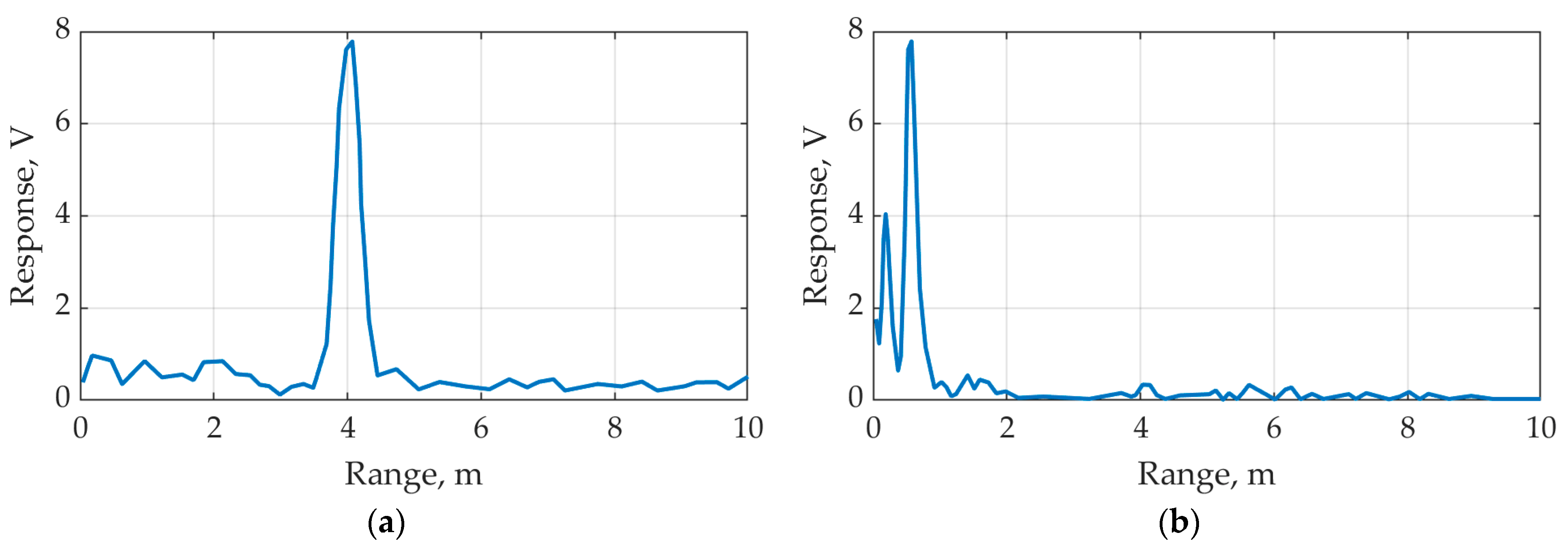
A typical curve of the real TRF measured when the target does not move is shown in
Figure 3a, where the probing was conducted in an open space (outdoors); (b), where there was a probing in a room through a brick wall 0.5 m thick. In both cases, the person was in the “standing still” position at a distance of 4 m from the radar antenna, and the parameters of the SFCW signal are the same as when they were used in the evaluation of the TRF shown in
Figure 2. The graphs in
Figure 3 show the values of the elements of one column, matching a single period with the number
k, of the vector
for range values
respectively (5).
As it can be seen in
Figure 3b, the SOI in the probing through the wall was much weaker (more than 20 times) than the signal produced by reflections from the wall. The latter was clear as two sharp peaks at ranges of about 0.1 m and 0.5 m corresponding to the signals reflected from the front and rear wall boundaries. The location of the peak related to the SOI at the range equal to 4 m could only be anticipated if the response shown in
Figure 3a had been known. Furthermore, the SOI just slightly exceeded the level of reflections from other objects in the room such as pieces of furniture, side walls, floor, ceiling, etc.
3. Signal Processing Algorithms
The selection of signals of moving or oscillating objects against the signals reflected from background and stationary objects was based on the identification of specific changes in complex samples or ordered by the slow time index k for each element taken out of the same range marked with the number n. The micro-displacements of the objects, whose values were just small fractions of the wavelength of the probing signal central frequency, led to such changes in complex samples that the modulus of their difference could significantly exceed both the average noise level and the corresponding difference in signals from stationary objects.
If the observation statistics implemented a nonlinear transformation function, e.g., the summation of modules or normalization of samples, then its application before or after the DFT operation would evidently lead to different results.
It is important to notice that when the problem of detecting mobile targets was to be solved, the number of samples involved should have been small. The typical value was from 3 to 10, which naturally corresponded to the observation time of no more than 0.5 s, during which the target remained within the same range resolution element under consideration.
3.1. Algorithm Based on Interperiodic Subtraction
The calculation of the interperiodic difference had historically been the first algorithm and still remains very effective among the class of algorithms designed for isolating mobile targets. In relation to the SFCW signal, it could be successfully performed over the samples
or
. It assumed the introduction of the matrix
V, containing samples of the difference signals
where
Switching to the range profile can be done by applying IDFT to the columns of the matrix
V. As a result, we get the matrix
where
.
During evaluation of the element of vectors , the order in which the different operations (7) and IDFT are applied could be reversed due to their linearity. It allowed one to calculate the element of matrix X using the Equation (7) where values are substituted instead of .
In the case where moving targets are to be detected, the elements of matrix
X were used to calculate the critical statistics by accumulating the energy of the observed signal in each range resolution cell:
where
K0 is the number of accumulation periods.
When K0 = 2, the columns of the matrix can be considered as a range profile where moving targets are being highlighted in each probing period with a number .
The resultant curve obtained via processing the samples
, where the choice of
K0 = 2 is made and the values
are involved, is shown in
Figure 4. The comparison between curves shown in
Figure 3b and
Figure 4 shows that using the interperiodic subtraction algorithm, the level of the signal of interest, corresponding to the target which is at a distance of 4 m, has significantly increased. Thus, the signal happens to exceed the reflection from the wall by about 4 times, i.e., by 6 dB, while the average level of interference from the stationary objects is lower by more than 15 times (or about 12 dB).
3.2. Algorithm Based on Local Variance
The absolute values of the differences in (9) at a fixed value n may still remain relatively small, especially if a target moves rather slowly or a small amplitude of its local oscillations occurs as well as if a level of the reflected signal turns out to be weak for any other reason. In this case, instead of simply summing up the differences, as it is done using the interperiodic subtraction algorithm, the estimation of the local variance can be conducted based on K0 > 2 slow time instants. The term “local variance” highlights the fact that the value , and the evaluation of the variance of samples for each fixed value n is actually carried out in a sliding window where .
The matrix made of the elements whose values are statistics calculated on the basis of matrix elements
G according to the local variance algorithm is determined as follows:
where
is a column vector with elements
The evaluation of the local statistics by means of Equation (11) makes it possible to utilize effectively the set of multiple samples belonging to frames in contrast to the statistics of interperiodic subtraction (9), yielding even with the same value K0. This is achieved by two proposals. First, the differences between the current values of the instant and their average value for K0 frames are used, and, second, the accumulation is not performed over the absolute values of the differences but over their squared values. The latter corresponds to energy-like accumulation that made the scheme more robust.
Basically, two important facts are to be highlighted regarding the statistics gathered by the two algorithms, interperiodic subtraction and local variance.
1. Element-wise evaluation of vectors of differences D(k) and V(k) involves complex-valued samples rather than their absolute values. Since the difference between the values of or ordered by the index k is likely to be determined by the amplitudes of the signals as well as by their phases, this important feature points out the effectiveness of the algorithms under consideration.
2. The signal processing carried out in accordance with Equations (6)–(9) for the interperiodic subtraction algorithm and (10)–(11) for the local variance algorithm corresponds to the methods of linear and quadratic accumulation of incoherent signals known in radar theory [
26]. The second of the above-mentioned methods is usually supposed to be more effective in the case where a signal of interest is assumed to be weak.
3.3. Algorithm Based on the Normalized Difference Samples of the SFCW Signal
The principal assumption leading the proposed algorithm based on normalized samples is the necessity of aligning the pulse amplitudes with the SFCW signal for all samples indexed by n = 1, …, N. Such alignment is aimed at compensating for the hardware shortcomings associated with the non-uniform amplitude-frequency characteristics of the transmitting and receiving paths. Consequently, it will reduce the undesirable amplitude modulation of the received signal and, thus, improve the overall signal-to-noise ratio. In addition, the normalization of samples will also lead to the alignment of strong and weak signals, regardless of the range and reflective properties of the corresponding objects.
According to its basic idea, the proposed algorithm is somewhat close to the local variance algorithm because it utilizes the differences between the current sample values and their average estimated over K0 frames. However, the fundamental difference here is the normalization of difference samples, which is carried out before the reconstruction of the range profile, i.e., before the IDFT is applied. In other words, this algorithm performs the operation similar to the range compression.
The algorithm for generating statistics based on normalized difference samples (NDS) can be briefly described as a sequence of the following transformations:
At first, the dc, or constant, component is reduced from the sample sequence
by calculating the differences:
where
. The local average value
is estimated based on
K0 subsequent frames. Thus, it takes on different values at each observation period numbered with
k =
K0,…,
K.
Then, each complex sample
undergoes normalization by its absolute value:
Then, the matrix consisting the normalized complex samples is assembled:
Finally, the elements of the matrix columns
are processed to reconstruct the matrix containing the elements describing the range profile:
where each column of the matrix
Z is defined as
the operation
denotes the element-wise absolute value, i.e., the matrix whose elements are obtained as results of calculating the absolute values of each element of the argument matrix
I.
The elements of matrix Z can be used in the evaluation of the statistics designed for reliable detecting or accurate measuring of the coordinates of targets in a similar way to the statistics considered for inter-periodic subtraction algorithms as the elements of matrix X or for local variance as elements of matrix D. However, if the normalization operation (13) has been excluded, the outputs of the local variance and NDS algorithms will inevitably coincide.
The use of a normalized difference sample, which are the elements of matrix Z, allows one to improve the SNR in comparison with the cases where the statistics of inter-periodic subtraction and local variance are primarily exploited. This result has been confirmed by numerous experimental data from the radar system when observing single and multiple moving and stationary targets and described in more detail in paragraph 5. Despite the fact that there is still no rigorous theoretical substantiation supporting the advantages of the proposed method of processing SFCW signals found so far, the next section presents the results of computer modeling of the simple signals, for which quantitative estimates of the gains have been achieved in the form of a valuable SNR gain.
4. Computer Simulation Results
In order to evaluate the effectiveness of the proposed method involving sample normalization, we consider a simple model which includes the signal reflected by a single point reflector being observed in the presence of the hardware noise of the receiver in the background. At the same time, we are willing to take into account the typical conditions of technical forming and processing the SFCW signal by introducing an interfering amplitude modulation. This modulation can accurately simulate the non-uniform amplitude-frequency response of the transmitting and receiving paths as well as the undesired interference made by radio waves merely produced by signals which are reflected from closely located points of an ordinary multipoint target.
Thus, the model of the received SFCW signal can be written in the form of a set of
N discrete samples in some
k-th probing period as
where
is random amplitude coefficients of the SFCW signal samples,
is the time delay of the target signal located at the range
Rt,
is the initial phase, depending on the distance to the target and including the random component
, that occurs when the signal is reflected from the target, and the last term
denotes complex samples of white Gaussian noise with zero mean and variance
;
n = 0,…,
N is the “fast time” index.
During this statistical modeling, the SNR values are being estimated numerically based on values which, in turn, are calculated after performing IDFT on the SFCW signal. Both options—the absence and presence of sample normalization procedure—are considered. The following parameter values were chosen for the SFCW signal: f0 = 1 GHz, Δf = 1 GHz, N = 500, Δt = Ts/N = 10−5 s. The frequency relating to the acquisition of discrete samples taken out of the complex exponent in (18) is chosen to be fp = Δfτ0/Δt = 4 kHz, that corresponds to the maximal target range Rt = 6 m, or as the time value τ0 = 4 × 10⁻⁸ s. The variance of the noise is chosen , which yields the additional average amplitude value of the SFCW signal samples , that corresponds to SNR q = 6 dB.
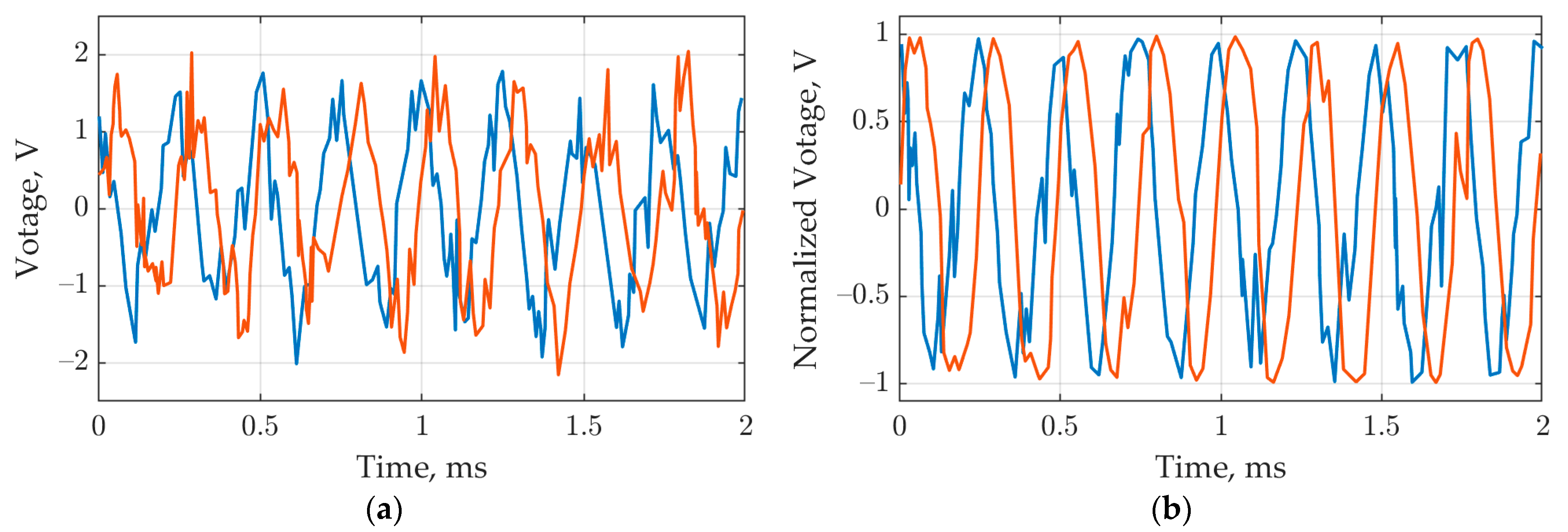
Figure 5 depicts the values of discrete samples (in the form of continuous lines for the sake of clarity) of the initial interval of the SFCW signal with a duration of 2 ms in the absence (a) of and in the presence (b) of the sample normalizing procedure. The real and imaginary parts of the complex-valued curves are illustrated by solid and dashed lines, respectively.
As can be seen, the sample normalization has led to the elimination of amplitude modulation simultaneously successfully mitigating the noise component of the signal.
The results of IDFT compression of the processed SFCW signals are shown in
Figure 6, where the abscissa axis is marked by frequency values in Hertz, and the amplitude spectra have been normalized to their maximal values.
Analyzing the curves in
Figure 6a,b, we would like to point out the fact that when the sample normalization was applied (b), the SNR value became noticeably higher. More accurate estimates obtained by averaging the results in a reliable statistical modeling manner has shown that, in the case under consideration, the gain in the SNR reaches about 3 dB (or twice). The results of the vast statistical modeling carried out over the wide range of parameters to establish the value of the SFCW signal and noise, reasonable from the technical point of view, showed that the value of the gain in SNR varies from 1 to 5 dB. It noticeably depended on the input SNR value and tended to increase with the growth of this value.
The results of conducted computer simulation merely relate to the analysis of the initial SFCW signals; however, we saw them preserved when we used other statistics, inter-periodic difference and local variance, while NDS was applied to the sample differences rather than samples themselves.
5. Results of Field Experiments
The set of full-scale field experiments was carried out using a radar system prototype developed at Scientific Research Center “PRLS”. A special testing room of 80 m2 total area was assembled with a brick wall of 0.5 m thick. During the experiments, the following parameters of the emitted SFCW signal were set: initial frequency f0 = 1 GHz, frequency change step Δf = 4 MHz, which give final frequency fN−1 = 2.5 GHz for the number of pulses N = 375, the duration of one pulse Δt = 50 μs, probing period Tr = 0.1 s yielding the frame rate 10 Hz. Thus, the maximum unambiguous range Rmax = 37.5 m, and the range resolution ΔR = 0.1 m can be found using (1).
All the experiments were conducted for the purpose of analyzing and comparing various signal processing algorithms that could be used to detect and measure the range of humans inside a controlled room. In all the experiments, the observation duration was set to 40 s, which corresponds to the number K = 400 frames, during which the complex samples were recorded in the radar system memory as the two-dimensional matrix (3). Signal processing can be implemented both using the built-in radar software and on a versatile personal computer.
The digital samples stored as the elements of the matrix S were processed using the algorithms described in paragraph 3, i.e., the inter-periodic subtraction, local variance and NDS, which all are designed to detect moving and oscillating targets. Two-dimensional matrices Y, D, Z were formed as the outputs of those algorithms. The number of averaging frames K0 = 5, corresponding to averaging time K0Tr = 0.5 s, was set for the second and third one. The range profile restoration was performed by IDFT transformation with the number of points Np = 1024 for all three algorithms.
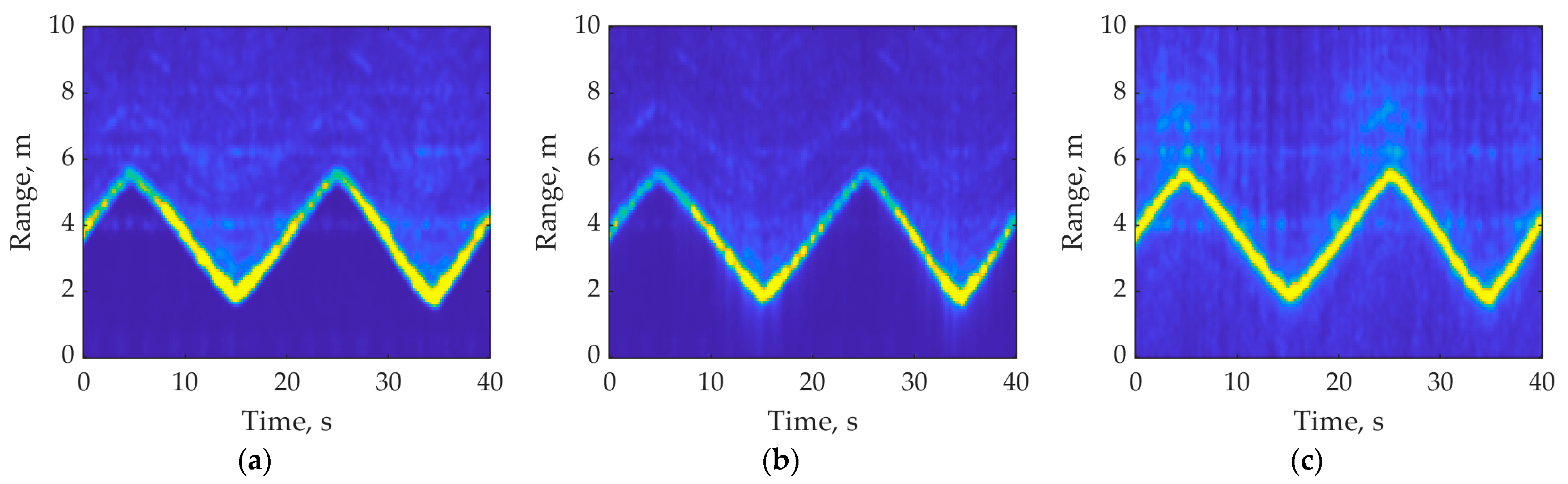
In the first experiment, during the entire observation period, a stationary person was standing still in a room at a distance of 4 m from the wall in a standing position facing the radar. The results of processing experimental data (elements of the matrix
S) are two-dimensional arrays
Y,
D,
Z, which are presented in the form of color images shown in
Figure 7, where the vertical axis corresponds to the range values at the interval (0, 10) meters (the range origin is the inner boundary of the room wall), and the horizontal axis corresponds to the instants of slow time
,
taken out of the interval (0, 40) seconds.
The signal of interest in all three figures is observed in the form of a horizontal intermittent line of a warmer tone passing along the range of 4 m. At the same time, one can notice that the line of the signal is the brightest in
Figure 7c, where the NDS algorithm was applied. Thus, the total contrast of the image (c) is much higher than in
Figure 7a,b where the algorithms of inter-periodic subtraction and local variance were applied without NDS.
The interfering clutters can also be observed in all images in
Figure 7. They appear as vertical stripes or individual spots. These interferences are caused by re-reflections of the signal of interest from other stationary objects in the room, such as pieces of furniture, walls, floor, ceiling, etc. It should be noticed that for the NDS algorithm, the level of interfering clutters is significantly less than for the interperiodic subtraction and local variance algorithms without NDS. The comparison between the pair –the interperiodic subtraction and local variance algorithms, which are shown in
Figure 7a,b respectively—reveals the undoubted advantage of the latter, which expresses a higher level of the overall brightness of the band corresponding to the signal of interest at a distance of 4 m.
The comparison described above is merely based on the visual perception of the images depicting two-dimensional signal matrices. Such a comparison remains important when the operator is assessing whether the situation required an urgent response, e.g., in the case of emergency; however, it is still a subjective assessment. The objective assessment leading to automated analysis and comparison of the target detection algorithms can be obtained if the calculation of the final statistics is carried out independently for each range by accumulating the difference signals of several frames. Those statistics, which are simply the sums of the row elements in matrices
Y,
D,
Z corresponding to the algorithms of interperiodic subtraction, local variance and NDS, are determined by the formulae:
where
denotes the number of the range element.
The evaluated cumulative statistics
are shown in
Figure 8 with dotted, dashed, and solid lines respectively as the curves against the index
n. Those lines are naturally related to the images in
Figure 7, presenting the valuable information in a compressed form. All three curves have been normalized to their maximum values in order to make a visual comparison easier.
The curves shown in
Figure 8 show that each of the three algorithms provides detection of the signal of interest reflected by the target at the distance of 4 m. However, the resulting values of SNR differ noticeably: 2 dB (in 1.6 times) for the interperiod subtraction algorithm, 3.7 dB (in 2.3 times) for the local variance algorithm, 6 dB (in 4 times) for the NDS algorithm.
Thus, in the conditions of the experiment under consideration, the NRS algorithm provides an improvement in the value of the SNR by 2.3 dB compared to the local variance algorithm and by 4 dB compared to the interperiodic subtraction algorithm. We can also point out that generally, in radar technique, a gain in the threshold SNR value of 2… 3 dB leads to an increase of the target detection range by about 1.5 times. Otherwise, it will preserve the detection performance for the target placed at the same distance if the wall thickness has been increased by almost the same ratio.
In the second experiment, two people remained in the room during the entire observation period. The first human stood still at the same range facing the radar, while the second was walking along the line of sight of the radar antenna within ranges to the wall changing from 2 to 6 m. The images depicting two-dimensional matrices
Y,
D,
Z for this experiment are shown in
Figure 9a–c respectively.
The line within ranges from 2 to 6 m in all images in
Figure 8 resembles the triangular pulse train and corresponds to the signal of interest reflected from a moving human. It can be additionally seen that the NDS algorithm provides a higher SNR, which is expressed as a larger amplitude (warmer colors) of the signal of moving and stationary targets. The latter reproduced the horizontal line at a range of 4 m. It can be noticed that the signal of the human who was not moving is much weaker than the signal of a walking person. The former is barely noticeable in
Figure 9c, even with the NDS algorithm applied. This signal is practically indistinguishable in the images obtained by means of the inter-periodic subtraction and local variance algorithms—
Figure 9a,b.
The poor “visibility” of the signal of a stationary person in
Figure 9 is explained by the fact that its level is significantly less than the signal of a walking person, and, consequently, the brightness of this signal in the image shifts to the region of lower values of the brightness range. However, such a signal can also be detected if the accumulation time is long enough by the accumulation technique similar to one implemented in
Figure 8.
It is important to notice here that, compared to the interperiodic subtraction and local variance algorithms, the NDS algorithm allows increasing the SNR in the case of the presence of moving and immobile people in the room, both separately or together, and, thus, it will generally improve the performance of their detector based upon it.
6. Discussion
The brief comparison between the radar prototype described in this work and other known radar systems emitting and processing SFCW signals are given in
Table 1. The comparison has deliberately been narrowed to the radar systems exploiting SFCW signals only since this class of radar systems is of the primary interest. A wider and more exhaustive comparison between state-of-art radar systems belonging to different classes with respect to their exploiting signals can be found in [
11]; in addition, some application-specific features of some systems are compared in [
41,
52]. Overall, the following parameters have been compared: frequency range (Freq), working distance (d), transmitter power (Tx Power), number of frequency steps (Steps), typical applications, declared usage in through wall scenario (TWR), main signal processing algorithms.
It is important to notice that regardless of the chosen probing waveform and processing algorithms for detecting people, there was always a threshold in SNR, i.e., the lowest value of SNR limiting the overall detection performance. Once the actual SNR reached this threshold, the performance of the method drastically deteriorated, making its usage no longer reliable. A clear demonstration of this behavior was given in [
55] where the SNR threshold was estimated as 8 dB for an UWB class on simulated data. The reasonable explanation of the phenomenon is originated in the correspondence of the measured data to the models which had been taken as the basis for algorithm design. In turn, the accuracy of parametric estimation of those models are limited, in general, by Cramer-Rao Lower Bound provided that model satisfies the regularity conditions [
56]. The latter usually assumes exploiting well-known linear processing algorithms, e.g., FFT or basic version of interperiod subtraction.
However, there is still a place for improving the overall performance of radar system if an appropriate ad hoc nonlinear method is inserted in the common signal processing framework. This work has demonstrated such a method tailored to processing the SFCW signals. It preserves the traditional sequence of signal processing steps including quadrature phase detection, inverse discrete Fourier transform and calculation of the interperiod difference of samples [
10,
19]. The proposed algorithm remains effective in cases where a detection of moving or stationary (not moving) human may be required since it shows performance in both cases.
7. Conclusions
The algorithm of processing the SFCW signal was described in the paper and it was proposed to include the step where the normalization of complex-valued samples by their own absolute values was carried out. The proposed signal processing method was intended for use in radar systems, in which the influence of interfering clutters and irregularities in the amplitude-frequency characteristics of the transmitting and receiving paths affects the received reflected signal due to the fact that the probing SFCW signals are ultra-wide band. The most significant effects caused by both factors consist in the appearance of unwanted amplitude modulation of the samples of the SFCW signal. It was shown that introducing normalization as a procedure applied to the samples of the SFCW signals or their inter-periodic differences made it possible to eliminate the undesired amplitude modulation due to the hardware signal path. Thus, it improved the overall SNR compared to the processing scenario where the SFCW signal was performed without the normalization step.
The results of computer modeling carried out to analyze the signal of a single point target showed that applying the method of normalizing of the differences of the sampling (NDS) to the reflected SFCW signal would lead to a gain of 1…5 dB in the SNR compared to the methods of interperiodic subtraction and local variance. The exact value of the gain had a tendency to go up if the input value of the SNR increases.
The field experiments were conducted with the multifunctional prototype of the radar system fully assembled in the University research center. The prototype successfully conducted all the required operations, including forming and converting the samples of the SFCW signal, putting them in and taking them out of the memory, quadrature detection, weighting and range compression using IDFT as well as displaying the information and general system control. The results of the field experiments showed the ability to reliably detect moving and stationary people through a brick wall of 0.5 m thick with the following main parameters of the SFCW signal: bandwidth was 1.5 GHz and an initial frequency was 1 GHz. The gain in the SNR provided by utilizing the proposed procedure was in the range of 2… 4 dB. The images depicting the absolute values of two-dimensional signal matrices as colored pictures for three processing algorithms—interperiodic subtraction, local variance and NDS were given. The warmer tone of the color highlighted the features introduced to the pictures by the signal of interest and is much higher over the background for the proposed NDS algorithm than for the first two algorithms, and the overall image contrast is also better.
The results obtained in this paper indicated the expediency of practical use of the NDS algorithm both in visual assessment of the situation, typically performed by an operator, and in automated mode as the fast signal processing was aimed at solving the problems of detecting human beings in critical situations and measuring their coordinates.


