Article

Duan–Rach Approach to Study Al2O3-Ethylene Glycol C2H6O2 Nanofluid Flow Based upon KKL Model

by
Pradyumna Kumar Pattnaik
1,
Satyaranjan Mishra
2 and
Muhammad Mubashir Bhatti
3,4,5,*
1
Department of Mathematics, College of Engineering and Technology, Bhubaneswar 751029, India
2
Department of Mathematics, Siksha ‘O’ Anusandhan Deemed to be University, Bhubaneswar, Odisha 751029, India
3
College of Mathematics and Systems Science, Shandong University of Science & Technology, Qingdao 266590, China
4
Shanghai Institute of Applied Mathematics and Mechanics, Shanghai University, Shanghai 200072, China
5
International Institute of Symmetry Analysis and Mathematical modeling, Department of Mathematical Sciences, North West University, Mafikeng Campus, Mmabatho 2735, South Africa
*
Author to whom correspondence should be addressed.
Inventions 2020, 5(3), 45; https://doi.org/10.3390/inventions5030045
Submission received: 12 July 2020 / Revised: 19 August 2020 / Accepted: 20 August 2020 / Published: 24 August 2020
(This article belongs to the Special Issue Recent Trends in Nanofluids - II)

Abstract

:
This work explains the cooling capabilities of ethylene glycol (EG)-based nanofluid containing aluminum oxide (Al2O3) as nanoparticles. Because of its enhanced thermophysical properties, Nanofluids are used in many application areas of mechanical and engineering in the form of nanofluid coolants such as electronics and vehicle cooling, transformer, and computer cooling. Depending on the heating and cooling systems, it is also used as an anti-freezing agent, which lowers the freezing point but enhances boiling point and temperature coolant. After using appropriate similarity transformation, the present Koo–Kleinstreuer–Li model for solving the boundary value problem (BVP) is tackled analytically. A comparison is made with a purely analytical approach by a modified version of the semi-analytical Adomian Decomposition Method (ADM), which is introduced by Duan and Rach (Duan–Rach Approach) and shooting technique. Analytical and graphical treatment of the flow regime is carried out, and the behavior of the leading parameters on the velocity, temperature, concentration profile with the behavior of physical quantities i.e., skin friction coefficient, local Nusselt number, and local Sherwood number are illustrated. This study confirms that, due to extraction in width the flow moves away from the lower plate whereas it moves towards near the upper plate and a rapid decrease in temperature is marked when alumina–EG nanofluids are taken into account.

1. Introduction

The mechanical processes of several industries vested upon the two vital aspects i.e., heating and cooling processes. The traditional heat transfers via phenomena through conventional fluids such as water, oil, etc. has poor conductivity as compared to the recent use of nanoparticles. The Nano-sized particles (1–100 nm) have a high thermal conductivity, which will enhance the thermal transfer properties. Both metals like copper, silver, aluminum, gold, etc. and metal oxides i.e., titanium oxide, alumina, copper oxide, etc. can be used as nanoparticles, submerged into the base fluids like water, kerosene, ethylene glycol forms nanofluid. It has an essential role in air conditioning, transportation, and many other industrial sectors. The pioneering work on nanofluids was obtained by Choi [1] in 1995; he started his work at the Argonne National Laboratory, USA. Various thermophysical properties are compared with base fluids like oil/water [2] and found that nanofluids have enhanced heat transfer capacity.
Ethylene glycol (EG) has IUPAC named as ethane-1, 2-diol, an organic compound, and its chemical symbol (CH2OH2). So, in the production process of polyester fibers, EG can be used in the raw material. It can also be used as an anti-freezing agent to reduce the freezing point of a water-based nanofluid, which, in turn, enhances the boiling point and coolant temperature of the nanofluid, automobiles and liquid-cooled computers. It has no odor, no color, but is a sweet-tasting viscous liquid. Because of these above properties, it is applicable in internal combustion engines and solar water heaters and HVAC chillers. This is also used in commercial purposes both in the pure concentrate and the diluted solution form, depending on the context.
This empowers a wide temperature to extend, which is fundamental to proficient heat transfer and the best possible working of heat exchangers. Applications of heat transfer incorporate in various types of consumption and are hostile to cavitation operators. Generally, it is also used in chilled-water cooling structures that are located in air handlers or chillers or structures that must cool under the frosty water’s temperature. It recovers vitality from water well, sea, and lake, and so forth, or scatters heat to the sink, contingent upon warming or cooling of the framework. These above facts of Ethylene glycol motivate us to adopt it in our research work.
Many researchers have shown their interest in investigating the different behaviors of Magnetohydrodynamics (MHD) and nanofluids in their respective regions because of the wide applications in engineering and biomedical areas. Barik et al. [3] utilized Finite difference method to solve nanofluid flow in an inclined and radiative stretching surface with multiple slip effects and showed its applications in microelectromechanical systems, and nanoelectromechanical systems, etc. Mutuku [4] examined the Ethylene glycol nanofluids by contemplating as a coolant for an automotive radiator. Mishra et al. [5] analyzed the mass transfer process under chemical reaction over a viscoelastic heated surface. Magnetic heat transfer on a multiphase nanofluid flow past through a square cavity was studied by Alsbery et al. [6]. Mohammadein et al. [7] analyzed the effect of the magnetic field and thermal radiation effect on considering a CuO water-based nanofluid numerically. Rahimi et al. [8] used the Lattice Boltzmann scheme to discuss the three-dimensional natural convection motion in cuboid fluid with the dual-MRT model. Rout and Mishra [9] contemplated about the thermal energy and magnetic nanofluid to examine the stretching flow. Rana and Nawaz [10] investigated the Sutterby nanofluids with the Koo–Kleinstreuer–Lee (KKL) model under the heat transfer mechanism. Mohamed [11] studied the electrical features of nanofluids via an artificial neural network.
Peng et al. [12] examined, using a numerical method, about the MHD radiative nanofluid motion under heat transfer through rotating annulus in a horizontal direction. Prakash et al. [13] discussed the nanofluid motion with peristaltic phenomena under magnetic thermal radiation effects with temperature-dependent viscosity and presented an application associated with a magnetic biomimetic nano pump. Rout and Mishra [14] applied an analytical approach to examine the metallic oxide features of copper and titanium nanoparticles moving through a vertical surface. Al-khaled and khan [15] explored thermal aspects of Casson nanofluid with the suspension of Gyrotactic Microorganisms with variable thermal conductivity and temperature-dependent viscosity. Bhatta et al. [16] used a semi-analytical scheme to the time-dependent squeezing flow to examine the behavior of Ag and copper-based nanoparticles. Khan and Tlili [17] contemplated the bioconvection nanofluid flow with the Jeffrey model under the presence of gyrotactic microorganisms and activation energy. Zhang et al. [18] used the DTM-Pade scheme to examine the behavior of nanoparticles and gyrotactic microorganism with generalized magnetic Reynolds number. Bhatti et al. [19] studied the activation energy of nanofluid and bioconvection flow over a porous surface. Ghasemi et al. [20] presented the high efficiency decolorization of wastewater in their study with the use of Fenton catalyst. Mozaffari [21] discussed the stability of water-in-oil emulsion in his thesis on the rheology of Bitumen at the onset of asphaltene aggregation. Equation of state of lattice gases extraction using Gibbs adsorption isotherm was conducted by Darjani et al. [22]. Ellahi et al. [23] discussed the Study of Two-Phase Newtonian Nanofluid Flow Hybrid with Hafnium Particles. They studied the influence of slip parameters on the flow phenomena. Recently, Ray et al. [24] proposed a semi-analytical technique known as Homotopy Analysis Method for the nanofluid transport in multiple geometrical configurations using a revised Buongiorno model. Abbas and Hussain [25] used a statistical analysis to determine the mathematical modeling of entropy generation with magnetic effects.
Owing to the literature as mentioned earlier, we have arrived at a point where the goal is to use the Duan–Rach approach to examine the Al2O3–Ethylene glycol nanofluid with the KKL model. A comparison is also presented between the Duan–Rach approach and numerical scheme. The effects of the magnetic field and porosity are also contemplated. The impact of various significant outcomes is discussed with tables and graphs. The inclusion of buoyancy parameters (both thermal and solutal) in the momentum equation, heat source, and radiation absorption parameters in the energy equation boost the physical phenomena of ethylene-glycol based Al2O3 nanofluid.

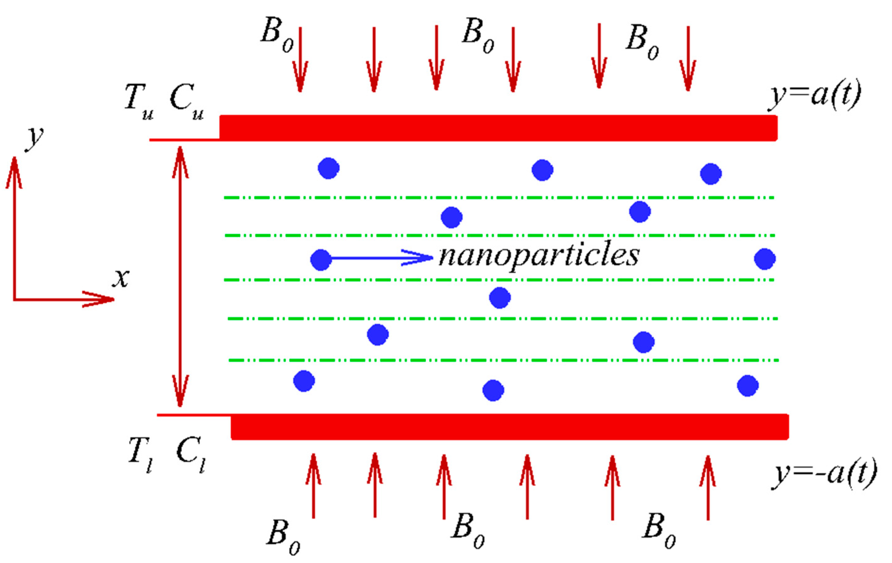
2. Mathematical Formulation

In the present problem, we have considered an unsteady two-dimensional MHD nanofluid flow past a permeable parallel channel, placed at a distance 2 a ( t ) apart, filled with porous. The influence of the external magnetic field is also applied in the transverse direction of the flow. Under the assumption of low magnetic Reynolds number, the induced magnetic field is assumed to be insignificant. We have taken EG as base fluid. External heat is imposed on the stationary wall that coincides with the x -axis, and the y -axis is normal. Therefore, the coolant of uniform velocity v w = a ( t ) is injected to the other end so that the plate will be transformed to cool i.e., either it will be expanding or contracting at a time-dependent rate. Due to the same reason, the flow is assumed to be a stagnation point of the flow (Figure 1). The present analysis of nano-solid particles and the base fluid is in thermal equilibrium, and no slip occurs between them where the existing base fluid is ethylene–glycol and nanoparticle is alumina. In Table 1, the thermophysical features of nanofluids are tabulated.
Following [26,27], the Navier–Stokes equations which governs the fluid flow may be written as:
D y v + D x u = 0 ,
D t u + u D x u + v D y u = 1 ρ n f D x p + υ n f 2 u ( σ B 0 2 ρ n f + υ f k p * ) u + g β T ( T T u ) + g β C ( C C u ) ,
D t v + u D x v + v D y v = 1 ρ n f D y p + υ n f 2 v ,
D t T + u D x T + v D y T = α n f 2 T Q 1 ( ρ c p ) n f ( T T h ) Q 2 ( ρ c p ) n f ( C C h ) ,
D t C + u D x C + v D y C = D 2 C ,
where
y = D y , x = D x , μ n f = μ f ( 1 ϕ ) 2.5 , ρ n f = ρ f ( 1 ϕ ) + ρ s ϕ , ( ρ c p ) n f = [ ( ρ c p ) f ( ρ c p ) f ϕ ] + ( ρ c p ) p ϕ .
The present model based upon the Koo and Kleinstreuer [28] thermal conductivity model, composed of both the static and Brownian motion part in which Brownian thermal conductivity play an import role on the thermal enhancement. Various particle sizes, temperatures, and volume fractions are accounted for using the same model, along with type of particles and base fluid combinations:
k e f f = k B r o w n i a n + k s t a t i c
k s t a t i c = { 1 + 3 ( 1 + K ¯ ) ( 2 + K ¯ ) ( 1 + K ¯ ) ϕ } k f
Here K ¯ = k p / k f , k s t a t i c is based on Maxwell classical correlation. The two most important empirical functions ( β and f ) defined in the model of Koo [29], the interaction between nanoparticles and the temperature impact reads as:
k B r o w n i a n = β ϕ 5 × 10 4 ρ f c p , f T κ b d p ρ p f ( T , ϕ )
where κ b , Boltzmann constant, and d p , diameter of the nanoparticle. The empirical g that depends upon the β and f (model of [30]).
For various nanoparticles, the function should be different. For ( Al 2 O 3 - C 2 H 6 O 2 ) nanofluids, this function is described as:
g ( T , ϕ , d p ) = ln ( T ) [ a 2 ln ( d p ) + a 1 + a 4 ln ( d p ) ln ( ϕ ) + a 3 ln ( ϕ ) + a 5 ln ( d p ) 2 ]   + [ a 7 ln ( d p ) + a 6 + a 9 ln ( d p ) ln ( ϕ ) + a 8 ln ( ϕ ) + a 10 ln ( d p ) 2 ] .
where ϕ 0.04 , 300 K T 325 K , and the coefficients a i , i = 0 10 comprise the nanoparticles’ type as depicted in discussion section.
The KKL correlation is described as:
k B r o w n i a n = c p , f ϕ ρ f k b T d p ρ p ( 5 × 10 4 ) g ( T , ϕ , d p )
The effective viscosity presented by Koo and Kleinstreuer [31] is modelled as
μ e f f = μ B r o w n i a n + μ s t a t i c = μ f Pr f k B r o w n i a n k f + μ s t a t i c
where the viscosity of the nanofluid, μ s t a t i c = μ f ( 1 ϕ ) 2.5 .
Using Equation (11) in Equation (12), the effective viscosity will be as:
μ e f f = μ s t a t i c + μ B r o w n i a n = μ f ( 1 ϕ ) 2.5 + k B r o w n i a n k f × μ f Pr f = μ f ( 1 ϕ ) 2.5 + μ f × 5 × 10 4 ϕ ρ f c p , f k f Pr f k b T d p ρ p g ( T , ϕ , d p ) .
The relevant boundary conditions:
y a ( t ) , u = 0 , v = v w = a ( t ) A 1 , T = T l , C = C l y a ( t ) , u = 0 , v = v w = a ( t ) A 1 , T = T u , C = C u } .
where A 1 = v w a ( t ) is the injection coefficient.
Since the proposed velocity function satisfies the continuity Equation (1), so it is very much compatible with the continuity equation. So, without loss of generality we have considered the stream function as ψ = x υ f a F ( η , t ) .
Following this, the similarity variable and dimensionless functions are:
η = y a , T u + θ ( η ) ( T l T u ) = T , ( C l C u ) χ ( η ) + C u = C .
We can obtain from Equations (2)–(6),
υ n f υ f ( F η η η η F η η K p ) + F η η F η + α [ η F η η η + 3 F η η ] M ρ f ρ n f F η η F F η η η a 2 υ f F η η t + λ 1 θ η + λ 2 χ η = 0
a 2 θ t + θ η F α η θ η S θ R a χ α n f υ f θ η η = 0
D χ η η a 2 χ t + υ f ( F α η ) χ η = 0
θ = 1 , F = Re , χ = 1 , F η = 0 at η = 1 θ = 0 , F η = 0 , χ = 0 F = Re , at η = 1 }
where Re = a v w υ f : Reynolds number.
The wall expansion ratio α is defined by the following:
α = a ˙ a υ = a ˙ 0 a 0 υ = constant
Depending on the physical situation of the present problem, it is observed that the model is based upon decelerating relaxation rate.
It is important to mention here that the wall expansion will be expanded for positive values and contracted for negative values.
Integrating, one can get [32]:
a a 0 = 2 υ α t + a 0 2 a 0 = υ w ( 0 ) υ w ( t )
Furthermore, substituting f = F / Re and considering f ,   θ and χ as functions of η one can admit
θ t = χ t = f η η t = 0
So Equations (11)–(13) can now be expressed as,
υ n f ( f η η η η K p f η η ) υ f + α ( 3 f η η + η f η η η ) ρ f ρ n f M f η η ( f η η η f f η f η η ) Re + λ 1 θ η + λ 2 χ η = 0 ,
α n f υ f θ η η Re ( f α η Re ) θ η S θ R a χ = 0 ,
D χ η η υ f Re ( f α η Re ) χ η = 0 ,
where α n f = k e f f ( ρ c p ) n f .
Now Equations (15)–(17) in the nanoparticle volume fraction form as:
f η η η η + A V 1 ( α ( 3 f η η + η f η η η ) Re ( f f η η η f η f η η ) + λ 1 θ η + λ 2 χ η ) ( M A + 1 K p ) f η η = 0 ,
θ η η Pr f B V 2 ( ( Re f α η ) θ η S θ R a χ ) = 0 ,
χ η η S c ( Re f α η ) χ η = 0 .
where 1 A = 1 ( 1 ϕ ) 2.5 [ 1 ( 1 ϕ ) 2.5 + k B r o w n i a n k f Pr f ] ,   V 1 = ( 1 ϕ + ρ s ρ f ϕ ) ,
1 B = ( k s t a t i c + k B r o w n i a n k f ) ,   V 2 = ( ϕ ( ρ c p ) s ( ρ c p ) f + 1 ϕ ) .
The boundary conditions Equation (14) reduced to,
f = 1 , f η = 0 , θ = 1 , χ = 1 at η = 1 f = 1 , f η = 0 , θ = 0 , χ = 0 at η = 1 } .
where M = σ a 2 B 2 μ f , K p = a 2 k p * , λ 1 = G r x Re , G r x = g β T a 4 ( T l T u ) x υ f 2 , λ 2 = G c x Re ,
G c x = g β C a 4 ( C l C u ) x υ f 2 , Pr f = μ f ( ρ c p ) f ρ f k f , S = Q 1 a 2 υ f , R a = Q 1 a 2 ( C l C u ) υ f ( T l T u ) , S c = υ f D

3. Formulation of Physical Quantities

The local skin friction coefficient, Nusselt and Sherwood number are expressed as
C f x = Re C f = 1 ( 1 ϕ ) 2.5 [ 1 ( 1 ϕ ) 2.5 + k B r o w n i a n k f Pr f ] f ( 1 ) , N u x = N u Re = Re ( k s t a t i c + k B r o w n i a n k f ) θ ( 1 ) , S h x = χ ( 1 ) , )
where
C f = τ x y ρ f v w 2 = 1 ρ f v w 2 ( μ n f u y ) y = a ( t ) , N u = x k f ( T l T u ) ( T y ) y = a ( t ) , S h = x D ( C l C u ) ( C y ) y = a ( t ) ,

4. Formulation of Duan–Rach Approach

Describing the method, we have considered a third-order nonlinear differential equation as:
L u = g ( η ) + N u ,
with boundary condition:
u ( η 0 ) = a 0 , u ( η 2 ) = a 2 , u ( η 1 ) = a 1 , η 1 η 2 , η 0 , η 1 , η 2 , a 0 , a 1 , a 2 R
where L = d 3 d x 3 , linear differential operator N u , analytic nonlinear operator and g ( η ) , system input.
The inverse linear operator for a prescribed value ξ in the given interval can be,
L 1 ( . ) = η 0 η η 1 η ξ η ( . ) d η d η d η ,
So,
L 1 ( L u ) = u ( η 0 ) + u ( η ) u ( η 1 ) ( η η 0 ) 1 2 ( ( η η 1 ) 2 ( η 0 η 1 ) 2 ) u ( ξ )
Taking the inverse operator on both sides of Equation (29),
L 1 [ g ( η ) + N u ] = u ( η 0 ) + u ( η ) u ( η 1 ) ( η η 0 ) 1 2 ( ( η η 1 ) 2 ( η 0 η 1 ) 2 ) u ( ξ )
Differentiating Equation (32) and inserting η = η 2 then solving u ( ξ ) one can get,
u ( ξ ) = u ( η 2 ) u ( η 1 ) η 2 η 1 1 η 2 η 1 η 1 η 2 ξ η [ g ( η ) + N u ] d η d η .
Substituting Equation (32) into Equation (31) yields,
u ( η ) = u ( η 0 ) + u ( η 1 ) ( η η 0 ) + L 1 ( N u + g ( η ) ) + 1 2 ( η η 1 ) 2 ( η 0 η 1 ) 2 η 2 η 1 ( u ( η 2 ) u ( η 1 ) η 1 η 2 ξ η ( N u + g ( η ) ) d η d η ) .
All the known boundary values are incorporated into Equation (33) and the undetermined coefficient was replaced. Now decomposing the linear as well as nonlinear terms as:
u ( η ) = m = 0 u m ( η ) , N u ( η ) = m = 0 A m ( η )
where A m ( η ) = A m ( u 0 ( η ) , u 1 ( η ) , u m ( η ) ) , Adomian polynomials.
Equation (33) gives the solution components which can be determined by the following recursion scheme:
u 0 ( η ) = u ( η 0 ) + u ( η 1 ) ( η η 0 ) + L 1 ( g ( η ) ) + 1 2 ( η η 1 ) 2 ( η 0 η 1 ) 2 η 2 η 1 ( u ( η 2 ) u ( η 1 ) η 1 η 2 ξ η g ( η ) d η d η ) .
u m + 1 ( η ) = L 1 ( A m ) 1 2 ( η η 1 ) 2 ( η 0 η 1 ) 2 η 2 η 1 η 1 η 2 ξ η A m d η d η .

5. Implementation of the Method

In this work, the transformed governing equations are solved by using a modified form of Adomian Decomposition scheme [33,34] named DRA [35]. The solutions are compared with the numerical solution achieved by shooting scheme. As compared with other techniques, the Adomian Decomposition scheme is helpful to examine a solution without using any numerical scheme. In fact, resulting solutions in final form do not have any undetermined coefficients.
Without considering ξ , DRA can be applied in our work as follows:
Introducing operators 4 = d 4 d η 4 ( ) and 2 = d 2 d η 2 ( ) , Equations (20)–(22) can be expressed as:
4 ( f ) = A V 1 ( α ( 3 f η η + η f η η η ) Re ( f f η η η f η f η η ) + λ 1 θ η + λ 2 χ η ) + ( M A + 1 K p ) f η η = N 1 u
2 ( θ ) = Pr f B V 2 ( ( Re f α η ) θ η S θ R a χ ) = N 2 u
2 ( χ ) = S c ( Re f α η ) χ η = N 3 u
Use of inverse operators 4 1 ( ) = 1 η 1 η 1 η 1 η ( ) d η d η d η d η and 2 1 ( ) = 1 η 1 η ( ) d η d η reduces Equation (36) as,
f ( η ) = f ( 1 ) + ( 1 + η ) f ( 1 ) + f ( 1 ) ( η + 1 ) 2 2 + f ( 1 ) ( η + 1 ) 3 6 + 4 1 ( N 1 u ) .
Since, we do not have boundary values of higher order let us take f η η ( 1 ) , f η η η ( 1 ) . We will calculate these values by avoiding the use of a standard Adomian Decomposition Method, as it uses numerical methods. The accuracy of the solution of Equation (39) obtained by using DRA depends on the accuracy of f η η ( 1 ) ,   f η η η ( 1 ) . In our approach, we have applied the Duan–Rach scheme to derive an analytical solution.
Now using Equation (26) in Equation (39) one can get
f ( 1 ) = 1 ,   6 f η η ( 1 ) + 4 f η η η ( 1 ) = 6 3 [ 4 1 ( N 1 u ) ] η = 1 ,
and for
f η ( 1 ) = 0 ,   2 f η η ( 1 ) + 2 f η η η ( 1 ) = [ 3 1 ( N 1 u ) ] η = 1 .
where 3 1 ( N 1 u ) = d d η [ 4 1 ( N 1 u ) ] = 1 η 1 η 1 η ( ) d η d η d η .
Solving f η η ( 1 ) and f η η η ( 1 ) from Equations (40) and (41) and using Equation (39) we get,
f ( η ) = 1 + 3 ( η + 1 ) 2 2 ( η + 1 ) 3 6 + { ( η + 1 ) 2 2 ( η + 1 ) 3 4 } [ 3 1 ( N 1 u ) ] η = 1 + { 3 ( η + 1 ) 2 4 + ( η + 1 ) 3 4 } [ 4 1 ( N 1 u ) ] η = 1 + 4 1 ( N 1 u ) .
A similar argument yields,
θ ( η ) = 1 ( η + 1 ) 2 ( η + 1 ) 2 [ 2 1 ( N 2 u ) ] η = 1 + 2 1 ( N 2 u ) .
χ ( η ) = 1 ( η + 1 ) 2 ( η + 1 ) 2 [ 2 1 ( N 3 u ) ] η = 1 + 2 1 ( N 3 u ) .
Following initial guesses are chosen,
f 0 ( η ) = 1 + 3 2 ( η + 1 ) 2 1 6 ( η + 1 ) 3 .
θ 0 ( η ) = 1 1 2 ( η + 1 ) .
χ 0 ( η ) = 1 1 2 ( η + 1 ) .
In addition, solving recursive schemes with m = 0 ,   1 ,   2 , ,
f m + 1 ( η ) = { ( η + 1 ) 2 2 ( η + 1 ) 3 4 } [ 3 1 ( N 1 u ) ] η = 1 + { 3 ( η + 1 ) 2 4 + ( η + 1 ) 3 4 } [ 4 1 ( N 1 u ) ] η = 1 + 4 1 ( N 1 u ) .
θ m + 1 ( η ) = ( η + 1 ) 2 [ 2 1 ( N 2 u ) ] η = 1 + 2 1 ( N 2 u ) .
χ m + 1 ( η ) = ( η + 1 ) 2 [ 2 1 ( N 3 u ) ] η = 1 + 2 1 ( N 3 u ) .
by using Adomian Polynomials and some default values of the pertinent parameters (varies as on demand in respective graphs) of the study M = 1 ,   λ 1 = 0.01 ,   λ 2 = 0.01 ,   S = 1 ,   R a = 1 , K p = 0.1 , P r f = 6.2 ,   α = 3 ,   R e = 3 , S c = 0.78 ,   ϕ = 0.02 we have,
f ( η ) = 0.0854 + 1.4387 η 1 + 0.271 η 2 0.7457 η 3 0.28 η 4 + 0.6757 η 5 + 0.0977 η 6 0.3659 η 7 + 0.003 η 8 0.006 η 9 0.002 η 10 + 0.003 η 11 + 0.000003 η 12 0.00004 η 13 + 0.0000003 η 15 .
θ ( η ) = 0.5193 0.4764 η 0.0142 η 2 + 0.0434 η 3 0.0067 η 4 0.0441 η 5 + 0.0039 η 6 0.0296 η 7 0.00293 η 8 + 0.0098 η 9 + 0.00075 η 10 0.003 η 11 + 0.00003 η 13 .
χ ( η ) = 0.5017 0.48034 η 0.0266 η 2 + 0.0171 η 3 + 0.00089 η 4 0.0278 η 5 + 0.00071 η 6 0.0115 η 7 0.00095 η 8 + 0.0038 η 9 + 0.0003 η 10 0.0013 η 11 + 0.00001 η 13 .

6. Discussion

The two-dimensional time-dependent flow of nanofluid within a channel of finite width is conducted in the present problem. Both the plates are permeable so that external pressure will act upon the flow phenomena. The fundamental aspect of the manufacturing industries is the automotive cooling and heating of the system. Compared to conventional liquid like water, oil, etc., the nanofluid’s thermal conductivity is more effective in nature. Therefore, the present model based upon a Koo–Kleinstreuer–Lee (KKL) model for higher thermal efficiency. Al 2 O 3 –Ethylene glycol nanofluid is used in the present investigation. The thermophysical properties and the experimental values of the coefficients used in the function are exhibited in Table 1 and Table 2, respectively. However, the novelty of our study is the purely analytical solution by the Duan–Rach approach, which modifies the Adomian Decomposition Method (ADM) along with the comparative research obtained by using a numerical method. The behavior of the contributing physical parameters on the flow profiles is displayed via graphs, and computational results for the engineering coefficient are presented in tabular form. Moreover, validation of our result with the earlier study is obtained for the flow phenomena. It is seen that the outcome is satisfactory, i.e., both the profiles coincide with each other in special cases.

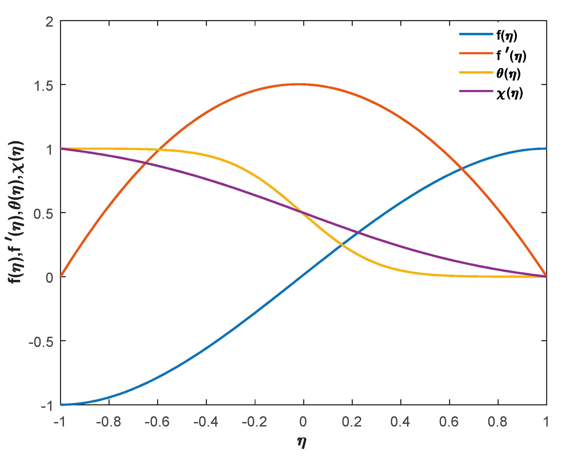
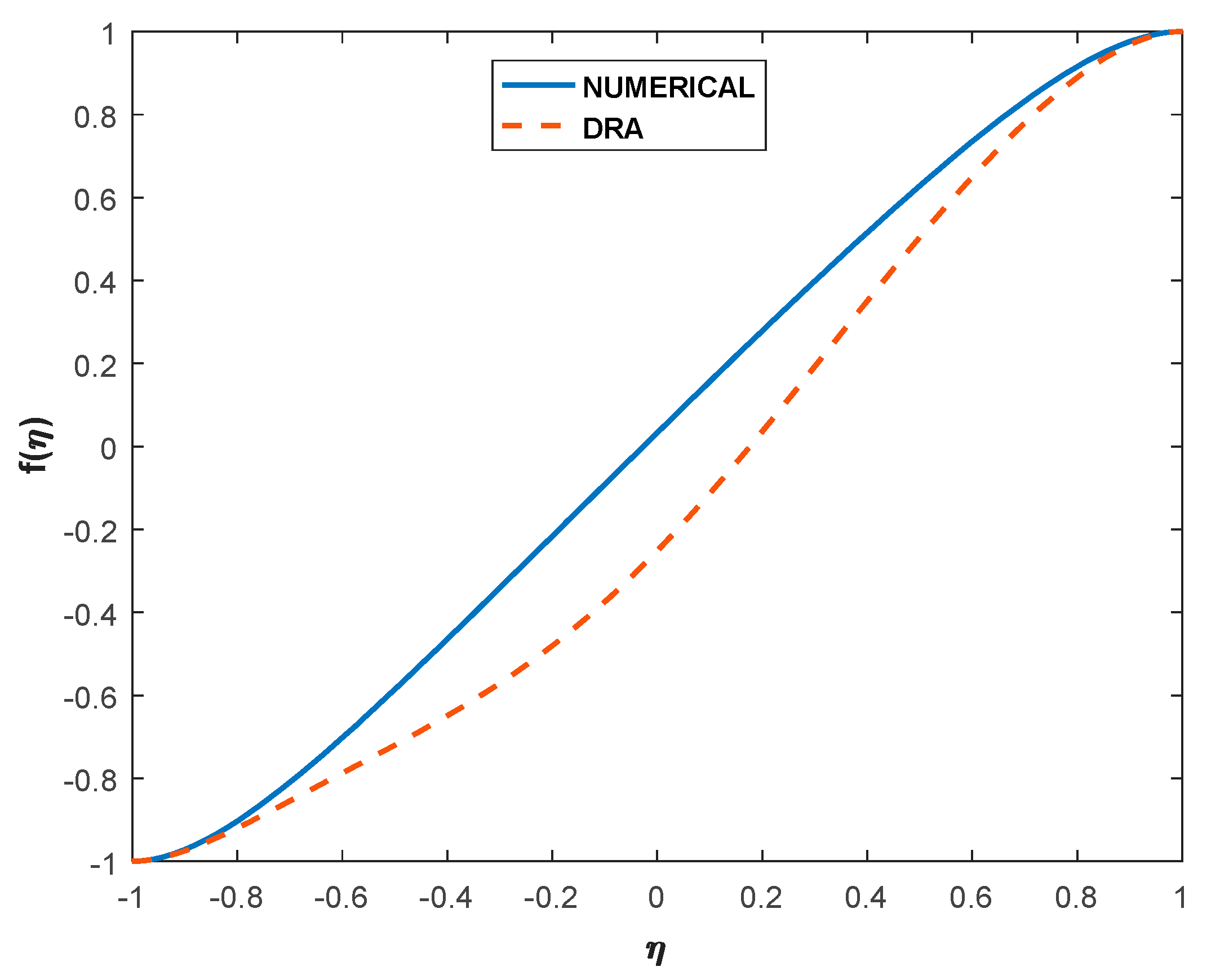
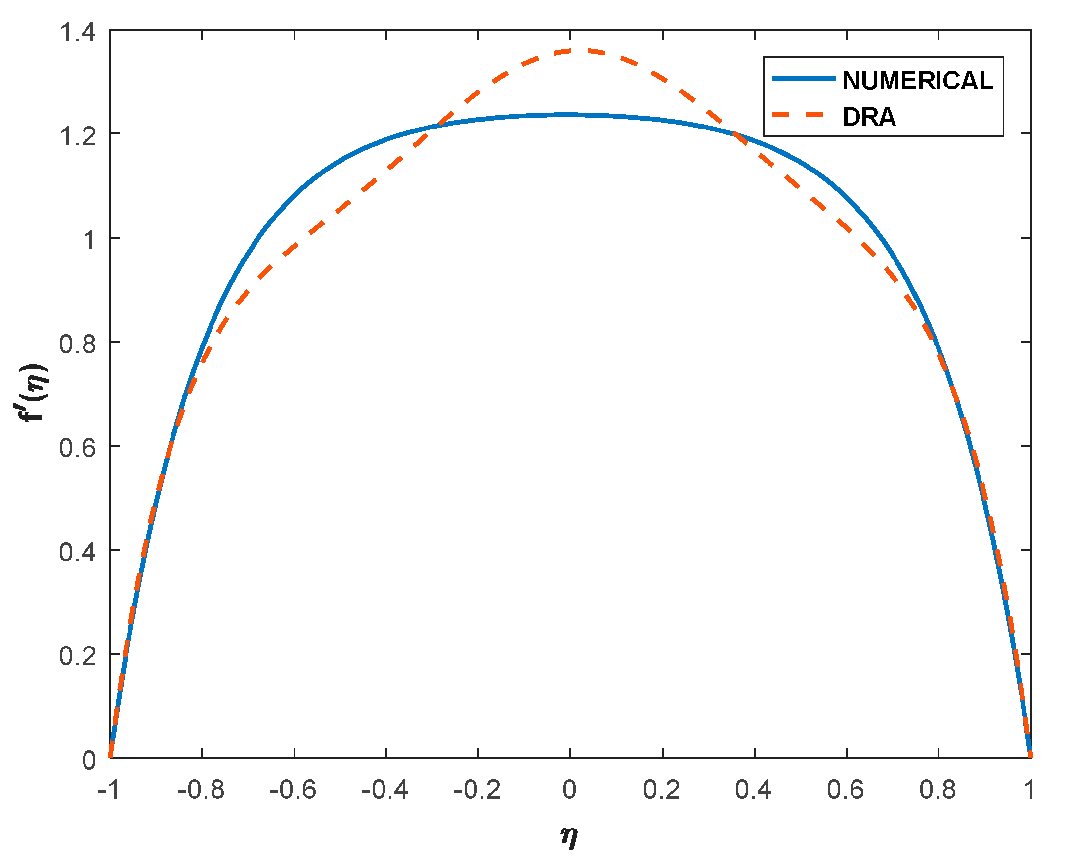
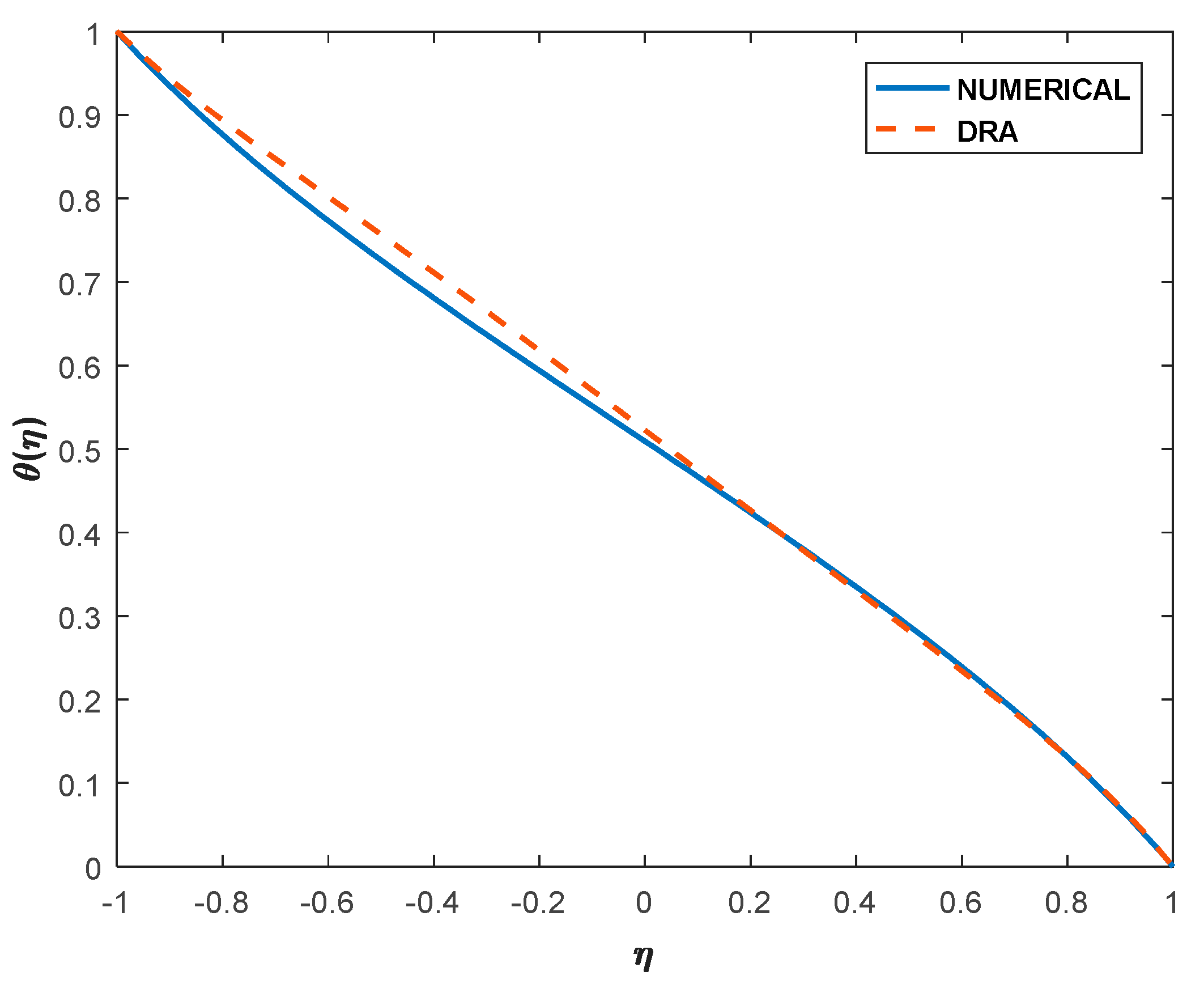
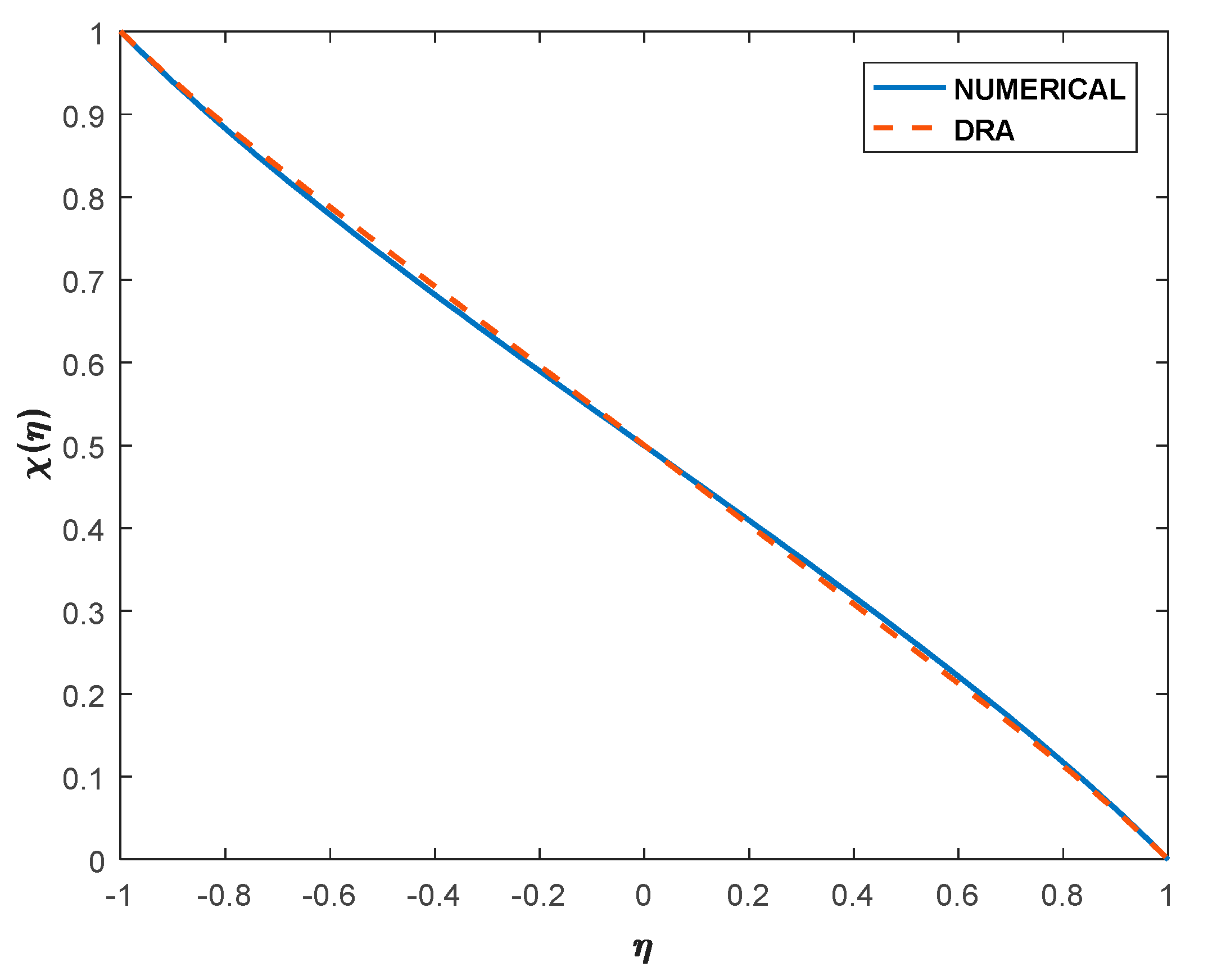
6.1. Validation and Comparative Study of Various Profiles

Figure 2 portrays the validation of stream function, velocity, temperature, and concentration profiles for the case of pure fluid i.e., the non-attendance of nanoparticle volume fraction ( ϕ = 0 ) . It is seen that in the case of pure fluid, the profiles coincide with the work of [36]. Moreover, the numerical outcomes by Runge–Kutta fourth-order method along with shooting technique, an analytical method using DRA for the stream function, is presented in Figure 3. The figure shows that both the numerical and DRA solution coincide with each other. Figure 4, Figure 5 and Figure 6 show the comparative results of the velocity, temperature, and concentration profiles for the aforesaid two methodologies. We arrived at the conclusion that both DRA and numerical approaches coincide with each other, showing the conformity of the convergence criteria.

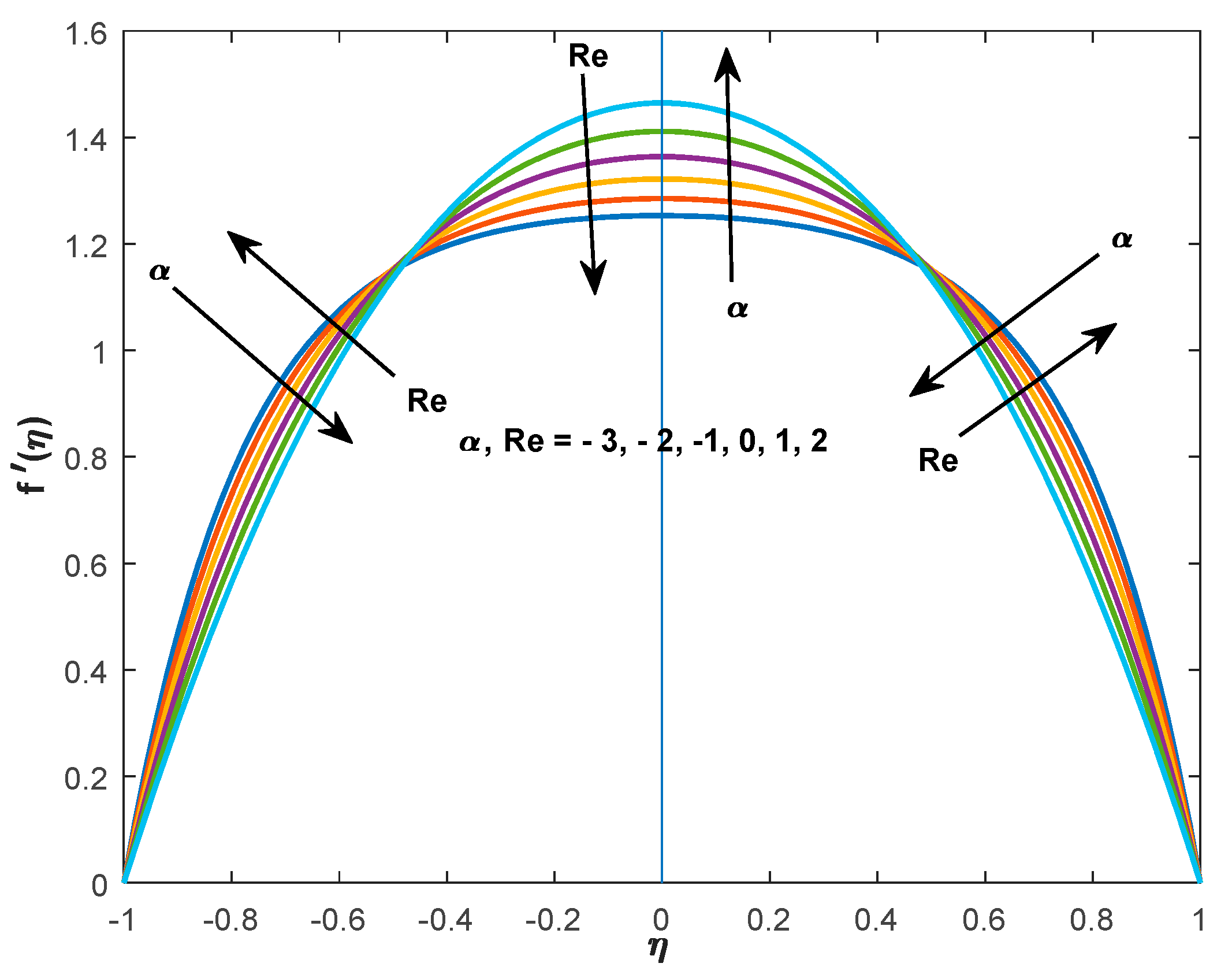
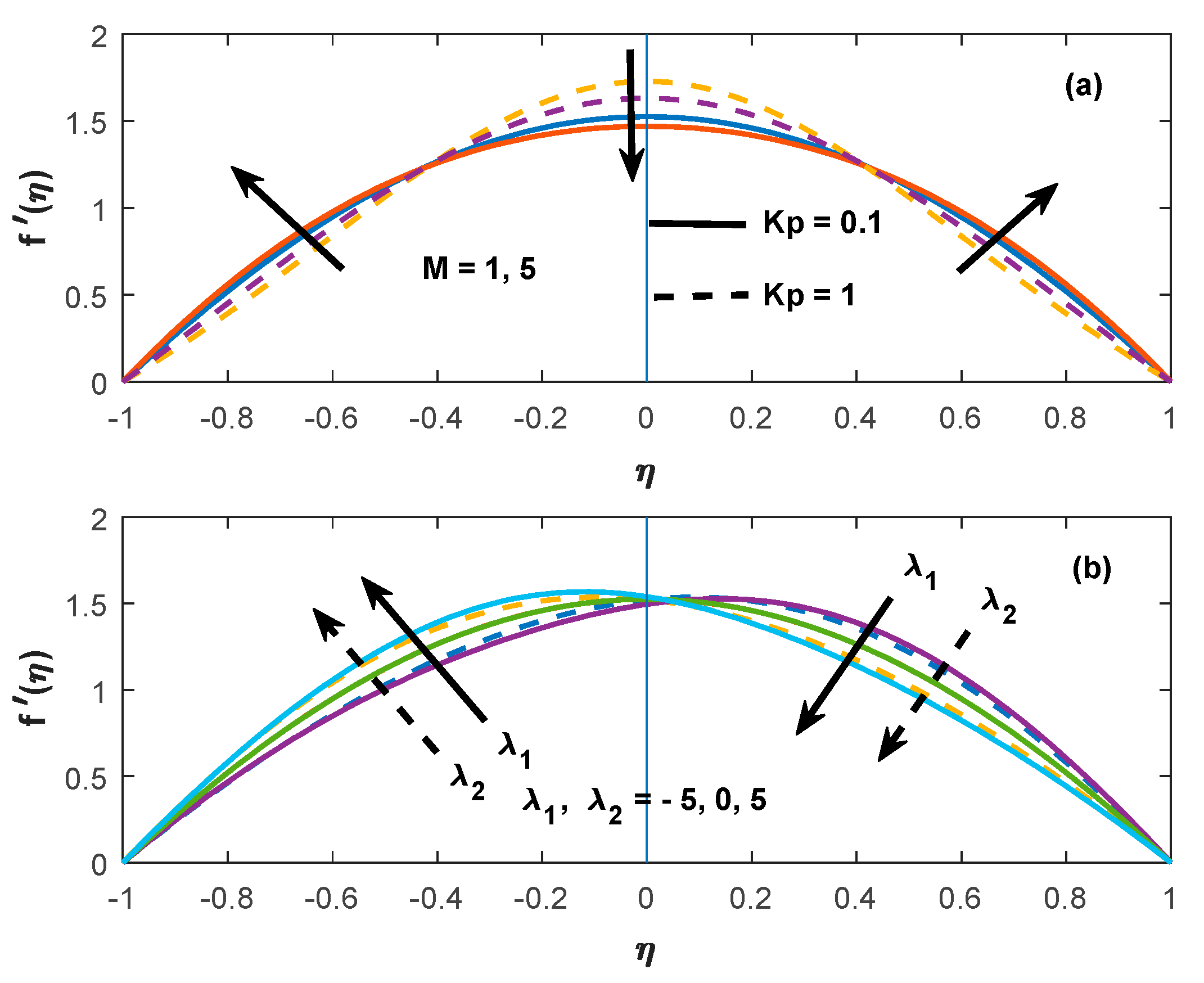
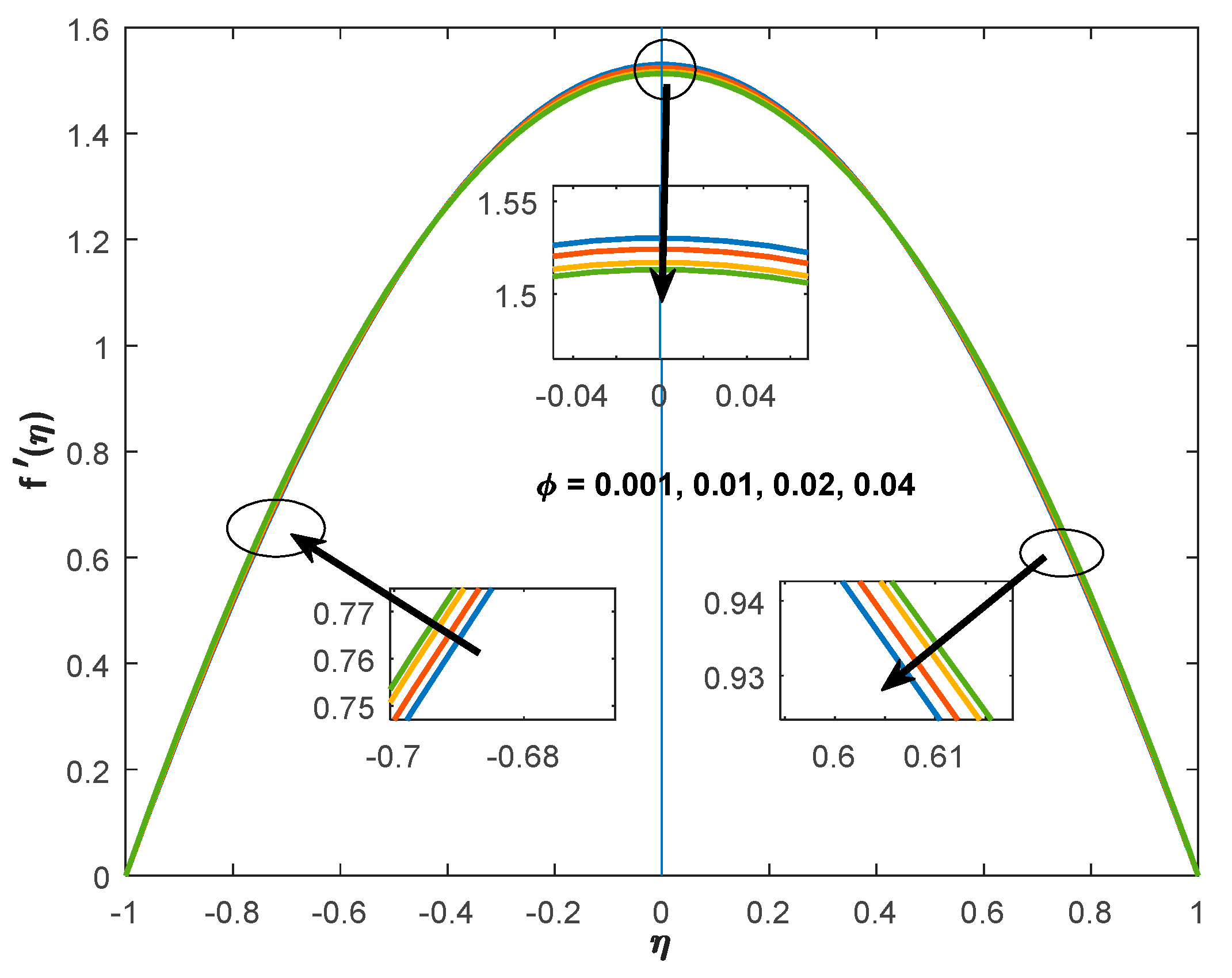
6.2. Variation of the Velocity Distribution

Figure 7 displays the variations of the wall expansion/contraction parameter and the Reynolds number on the velocity profiles. Three distinct characters in the profiles are exhibited in different regions of the channel, such as 1 η < 0.5 , 0.5 η < 0.5 and 0.5 η 1 . Near both the plate region (lower 1 η < 0.5 and upper 0.5 η 1 ), the higher magnitude in the Reynolds number decelerates the channel width. However, for an increase in channel width, the reverse behavior is encountered. In the middle layer of the channel, it is seen that the profile retards gradually, and increasing width overshoots the profile significantly. Due to extraction in width, the flow near the lower plate moves away from the plate, whereas the upper plate moves towards it. Figure 8 portrays the responsibilities of magnetic parameter and porosity as well as buoyant forces on the velocity distributions. In the Figure 8a, it is seen that the profile behaves symmetrically from the middle layer of the channel. However, at both the lower and upper plate regions, the thickness retards due to the increase in magnetic parameter and the middle layer of the profile also retards. The interaction of the magnetic parameter gives rise to produce a resistive force offered by the Lorentz force, which retards the fluid motion. Another underlying property is, due to the more massive density of the nanoparticles, the clogging is marked near the plate region; therefore, profile retards. The presence of a porous matrix overrides the velocity profile with magnetic parameter. Figure 8b presents the behavior of both the thermal and mass buoyancy on the velocity distributions. Here, λ 1 , λ 2 > 0 it presents the cooling and λ 1 , λ 2 < 0 shows the heating of the plate. It is observed that an increase in buoyancy forces from heating to cooling, the enhancing nature of the profiles exhibits to lower down the thickness at the lower plate in the region 1 η < 0 . Moreover, from the point of contact at the central region, the opposite effect is rendered near the upper plate region within the range 0 < η < 1 . Figure 9 illustrates the nanoparticle volume fraction on the velocity distribution. The amount of Al 2 O 3 nanoparticles from 0.01% to 4% in volume submerged into the ethylene glycol, and the effect is observed in the present case. It is found that increasing volume fraction retards the thickness at the lower plate; however, the upper plate’s expansion is more. The reason is that due to the heavier density of the nanoparticles, the clogging near the lower plate is greater. In the central region, a similar reduction is marked due to the increase in volume fraction.

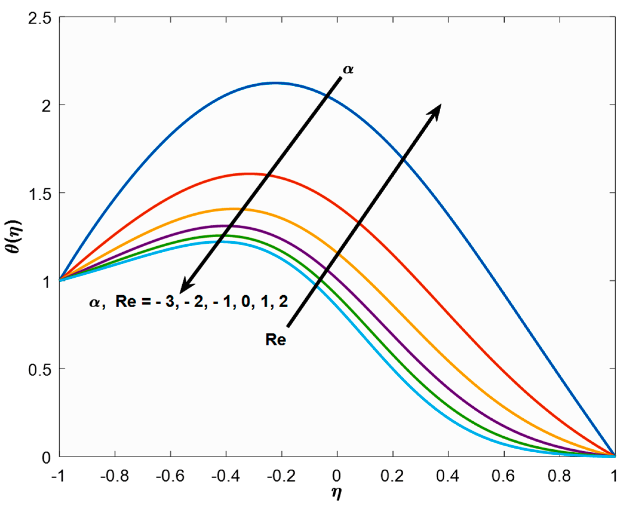
6.3. Variation of Temperature Distributions

Figure 10 describes the behavior of the extraction/contraction parameter along with the Reynolds number on the temperature distribution. It is seen that the profile overshoots with increasing suction and Reynolds number i.e., for positive values and reverse impact is rendered for the injection where it indicates the negative Reynolds number. The fact is, Reynolds number is associated with the coefficient of viscosity and is inversely proportional to it. When the nanofluid viscosity moves towards the viscosity of the suspending fluid medium, it assigns the Reynolds number’s negative values. Moreover, increasing contraction/extraction retardation in temperature profile has occurred. The variation of Prandtl number and the heat source/sink on the temperature profile of Al 2 O 3 –EG nanofluid is exhibited in Figure 11. The dual character is laid down for the various values of the Prandtl number on fluid temperature. In the region 1 η < 0 , the increasing Pr enhances the profile, whereas it decelerates in the region 0 η < 1 (Figure 11a). Prandtl number is inversely proportional to thermal diffusivity. Higher Pr means reduction in thermal diffusivity causes a suitable reduction in the profile. However, the variation of Re is well described in the previous profile. From Figure 11b, it is observed that heat source is favorable to enhance the fluid temperature in the complete domain further, reverse impact is rendered for the heat sink parameter. The volume factor presents its key behavior on the temperature profile since the conductivity of the medium helps to transfer the heat in the body. Therefore, the impact of volume fraction on the temperature is displayed in Figure 12. The peak in the profile is observed near the lower plate, and sudden fall is marked in the central region and further retards the profile at the upper plate region. The fact is, heavy clogging near the lower plate causes the reduction in velocity that described earlier at the same time; the stored energy rises, showing its increasing behavior. Moreover, due to the heavier density, the movement of particles from the upper plate towards the lower plate gives rise to a reduction in the profile at the upper plate region.

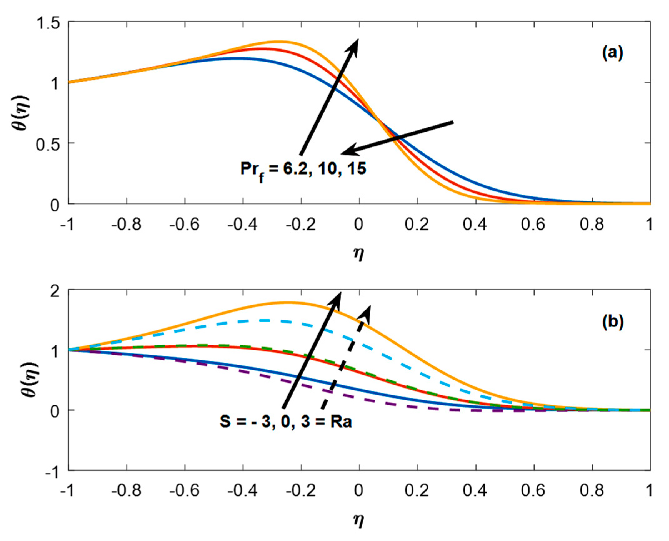
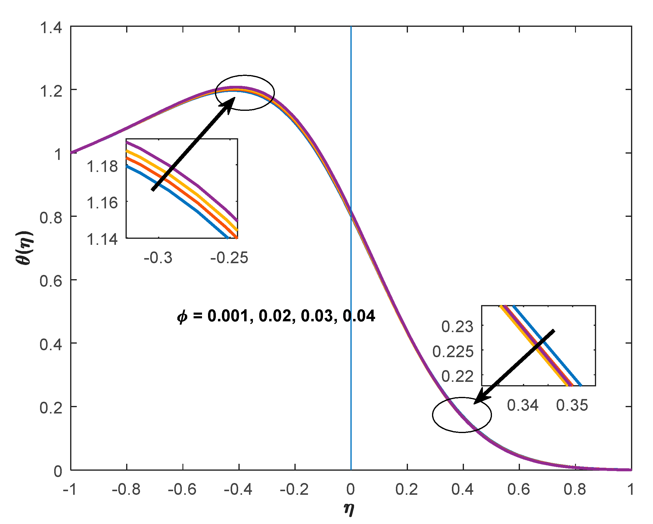
6.4. Variation of Temperature Distributions

The behavior of several characterizing parameters on the concentration profile is shown in the Figure 13 and Figure 14. Figure 13 illustrates the influence of α and Re on the concentration distribution. Two-layered variation is marked in the concentration profile due to the variation of this parameter from the central area of the channel. It is interesting to note that the point of inflection is marked in this region, and the profiles behave opposite in character. In the first region, enhance in Re retards the fluid concentration whereas for the contraction/extraction parameter favors in to improve the profile significantly. As described earlier, the impact is the opposite in the second region. The behavior of heavier species i.e., the Schmidt number on the solutal distribution, is marked in Figure 14. From the definition, it is clear that as mass diffusion reduces, the Schmidt number increases. Therefore, increasing S c the solutal distribution retards near the upper plate region.

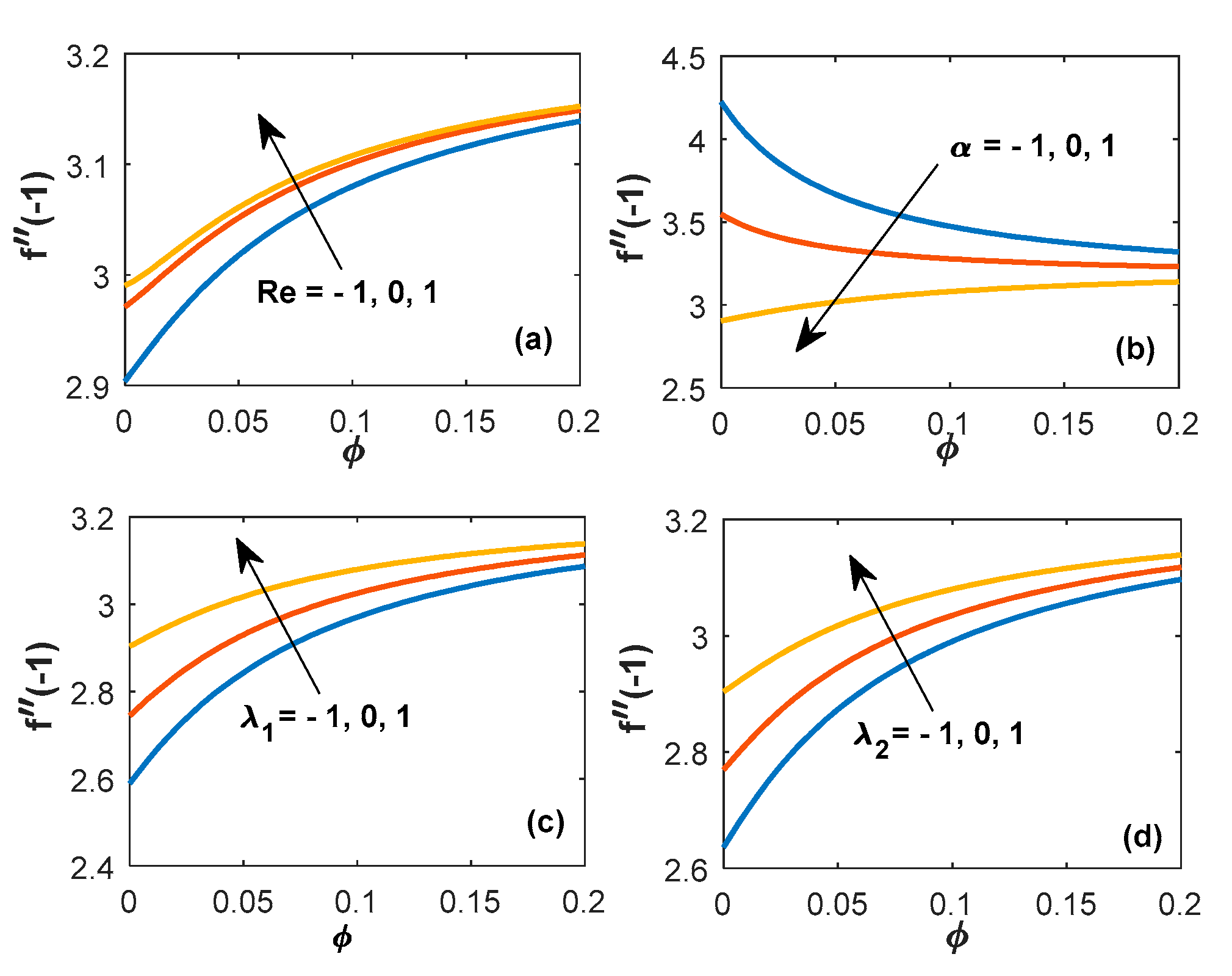
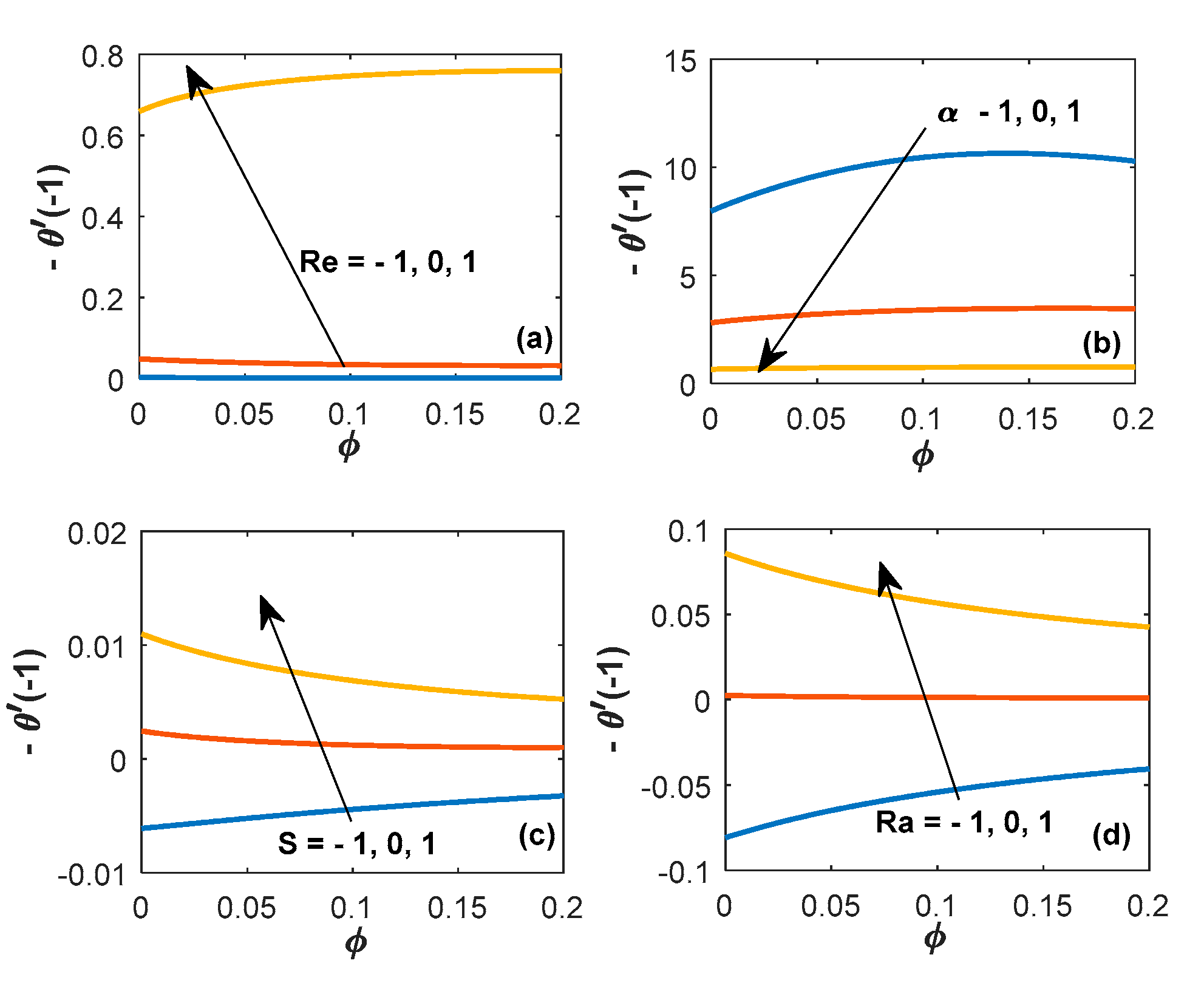
6.5. Variation of Engineering Coefficients

Finally, numerical simulation of thermophysical properties of various parameters on the rate of shear stress, Nusselt number, and the Sherwood number is displayed in Figure 15, Figure 16 and Figure 17. The influences of Re , α , λ 1 and λ 2 on the rate of shear stress coefficients at the lower plate are exhibited in Figure 15. These are observed for the various values of volume fraction. In this case, we have considered the number of nanoparticles as varying from 0% to 0.2%. It is observed that increasing Re and buoyant forces enhance the rate of shear stress, whereas remarkable retardation occurred due to the increase in the plate width. A similar tendency is rendered on the rate of heat transfer profiles i.e., for Nusselt number, which can be seen in Figure 16. Therefore, it is concluded that the growing volume fraction will cause a development in the heat transfer properties. Moreover, Figure 17 presents the rate of mass transfer i.e., the Sherwood number for the variation in Re , α and S c . It is observed that, both S c and α favors in to control the mass transfer within the fluid domain. Therefore, it is suggested that heavier species are useful in reducing the diffusivity rate, which has a significant impact in various industrial processes.

7. Conclusions

We have studied the ethylene glycol (EG)-based nanofluid containing aluminum oxide (Al2O3) as nanoparticles with the KKL model using the Duan–Rach approach. A comparison is made with a purely analytical approach by a modified version of the semi-analytical Adomian Decomposition Method (ADM), which is introduced by Duan and Rach (Duan–Rach Approach) and fourth-order Runge–Kutta method with shooting technique. Analytical and graphical treatment of the entire flow regime is carried out, and the effects of the pertinent parameters on the velocity, temperature, concentration profile with the behavior of physical quantities such as skin friction coefficient, local Nusselt number, and local Sherwood number are illustrated in the present work. The significant outcomes are explained below:
  • It is noticed that a rapid decrease in temperature profile is observed when Alumina–EG nanofluids are contemplated.
  • Porosity effects enhance the flow, whereas the magnetic field opposes the flow.
  • Increase in buoyancy forces from heating to cooling, the enhancing nature of the profiles exhibits to lower down the thickness at the lower plate in the half region. In contrast, from the point of contact at the central area, the opposite effect is rendered near the upper plate region.
  • It is found that increasing volume fraction retards the thickness at the lower plate; however, the expansion at the upper plate is more.
  • It is seen that the profile overshoots with increasing suction Reynolds number i.e., for positive values and reverse impact is rendered for the injection where it indicates the negative Reynolds number.
  • It is concluded that the growing volume fraction will cause a development in the heat transfer properties.
  • Prandtl number shows converse behavior in the upper region as compared with the low area.
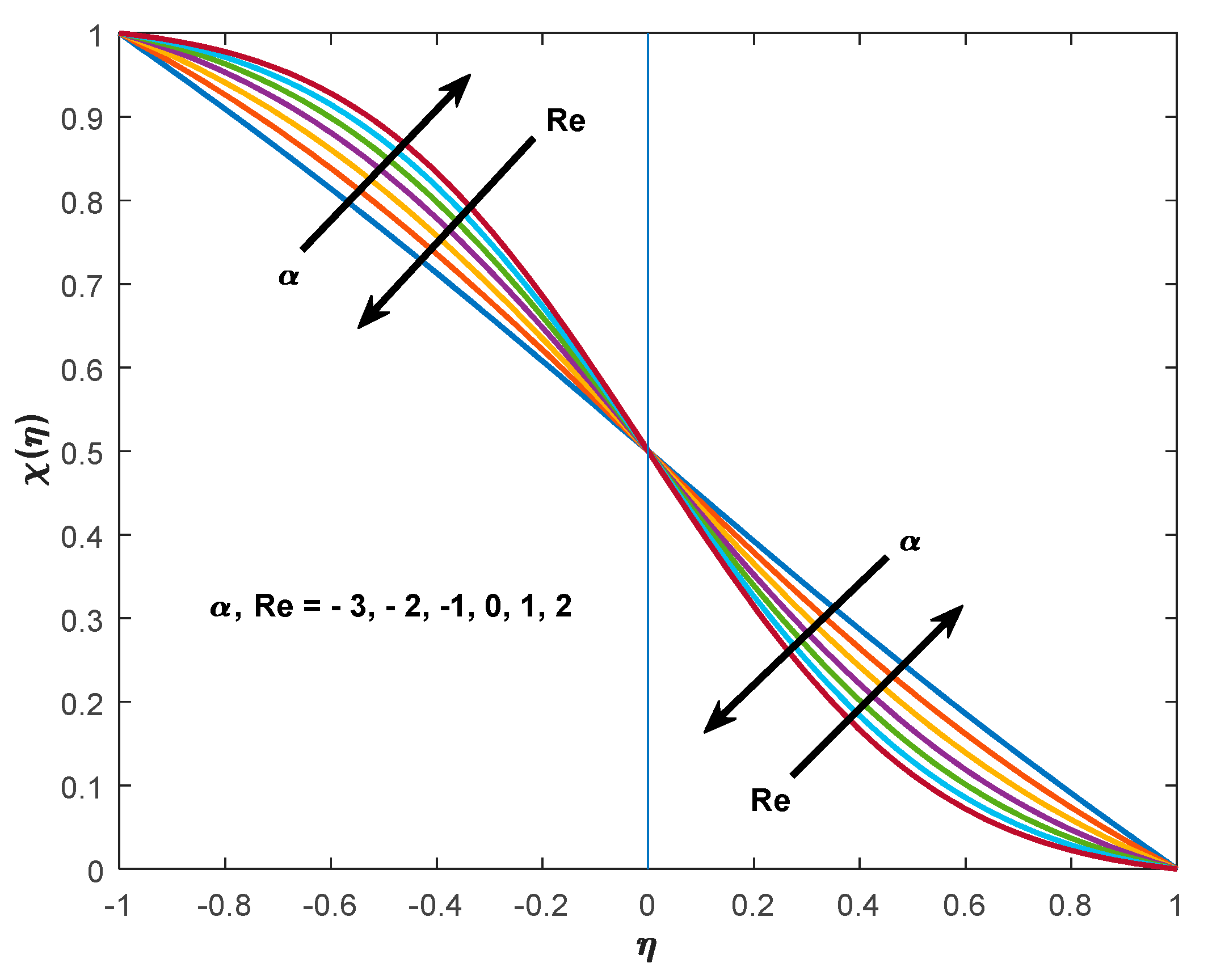
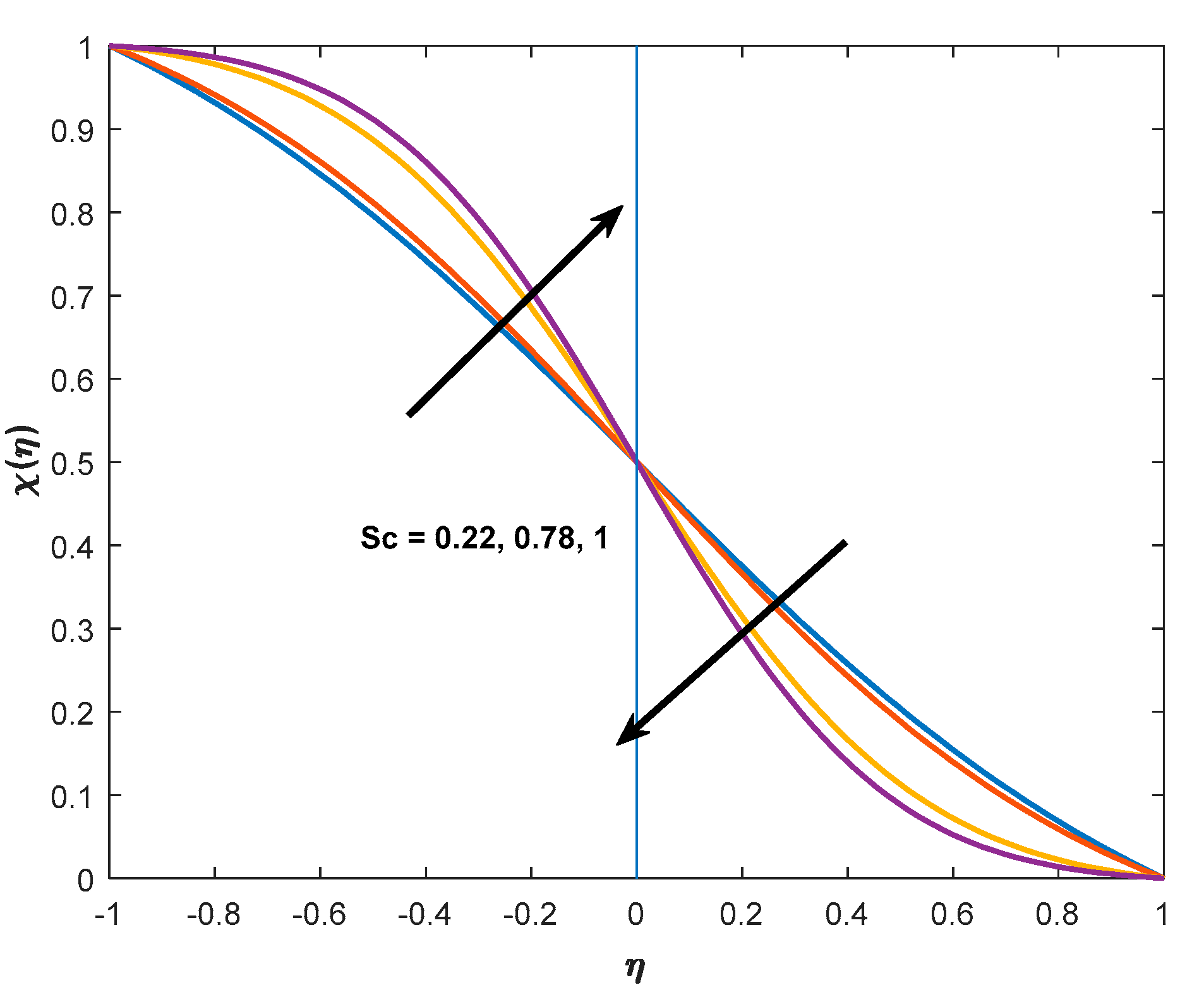
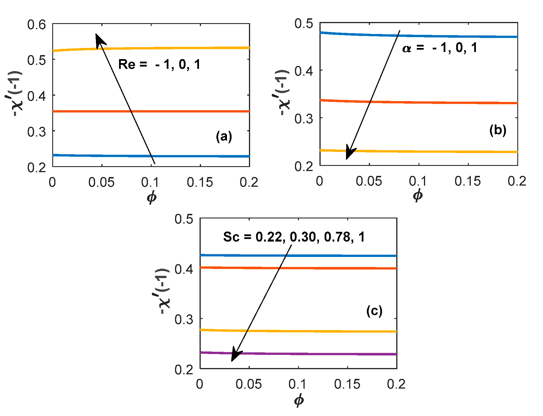
  • Reynolds number and Schmidt number show converse behavior on the concentration profile.

Author Contributions

Investigation, M.M.B. and P.K.P.; Methodology, P.K.P. and S.M.; Writing—review and editing, M.M.B.; Formal analysis, P.K.P. and S.M. All authors have read and agreed to the published version of the manuscript.

Funding

M.M.B. was supported by the Cultivation Project of Young and Innovative Talents in 193 Universities of Shandong Province (Nonlinear Sciences Research Team).

Conflicts of Interest

The authors declare no conflict of interest.

Nomenclature

A 1 Permeability
B 0 magnetic field strength
C concentration fluid
c p specific heat
D solutal diffusivity
f velocity profiles
F self-similar velocity
g gravity
n shape factor for nanoparticle
M magnetic parameter
k thermal conductivity of water
K p porosity parameter
( x , y ) horizontal and vertical co-ordinate axes
p pressure
Pr f Prandtl number
Q 1 heat source parameter
Q 2 coefficient of radiation absorption
R a non-dimensional radiation absorption
Re Reynolds number
S non-dimensional source parameter
S c Schmidt number
( u , v ) Horizontal and vertical velocity
T Temperature
Greek Symbols
ϕ nanoparticle volume fraction
ψ sphericity of the nanoparticles
υ kinematic viscosity
ρ fluid density
σ electrical conductivity
β T volumetric coefficient of expansion for heat transfer
β C volumetric coefficient of expansion for mass transfer
μ dynamic viscosity
α wall expansion/contraction parameter
α n f thermal diffusivity
η scaled boundary layer coordinate
θ dimensionless temperature
χ dimensionless concentration
λ 1 thermal buoyancy parameter
λ 2 solutal buoyancy parameter
( ρ c p ) heat capacity
Subscripts
nfnanofluid
fbase fluid
psolid particle
llower walls
uupper walls

References

  1. Choi, S.U.S. Enhancing thermal conductivity of fluids with nanoparticles. In Developments and Applications of Non-Newtonian Flows, FED-231/MD(66); Siginer, D.A., Wang, H.P., Eds.; ASME: New York, NY, USA, 1995; pp. 99–105. [Google Scholar]
  2. Choi, S.U.S. Nanofluids: From vision to reality through research. J. Heat Transf. 2009, 131, 1–9. [Google Scholar] [CrossRef]
  3. Barik, A.K.; Mishra, S.K.; Mishra, S.R.; Pattnaik, P.K. Multiple slip effects on MHD nanofluid flow over an inclined, radiative, and chemically reacting stretching sheet by means of FDM. Heat Transf. Asian Res. 2019, 1–25. [Google Scholar] [CrossRef]
  4. Mutuku, W.N. Ethylene glycol (EG)-based nanofluids as a coolant for automotive radiator. Asia Pac. J. Comput. Eng. 2016, 3, 1. [Google Scholar] [CrossRef] [Green Version]
  5. Mishra, S.R.; Pattnaik, P.K.; Bhatti, M.M.; Abbas, T. Analysis of heat and mass transfer with MHD and chemical reaction effects on viscoelastic fluid over a stretching sheet. Indian J. Phys. 2017. [Google Scholar] [CrossRef]
  6. Alsabery, A.I.; Sheremet, M.A.; Chamkha, A.J.; Hashim, I. MHD convective heat transfer in a discretely heated square cavity with conductive inner block using two-phase nanofluid model. Sci. Rep. 2018, 8, 7410. [Google Scholar] [CrossRef] [PubMed]
  7. Mohammadein, S.A.; Raslan, K.; Abdel-Wahed, M.S.; Abedel-Aal, E.M. KKL-model of MHD CuO-nanofluid flow over a stagnation point stretching sheet with nonlinear thermal radiation and suction/injection. Results Phys. 2018, 10, 194–199. [Google Scholar] [CrossRef]
  8. Rahimi, A.; Kasaeipoor, A.; Malekshah, E.H.; Rashidi, M.M.; Purusothaman, A. Lattice Boltzmann simulation of 3D natural convection in a cuboid filled with KKL-model predicted nanofluid using Dual-MRT model. Int. J. Numer. Methods Heat Fluid Flow 2018. [Google Scholar] [CrossRef]
  9. Rout, B.C.; Mishra, S.R. Thermal energy transport on MHD nanofluid flow over a stretching surface: A comparative study. Eng. Sci. Technol. Int. J. 2018, 21, 60–69. [Google Scholar] [CrossRef]
  10. Rana, S.; Nawaz, M. Investigation of enhancement of heat transfer in Sutterby nanofluid using Koo–Kleinstreuer and Li (KKL) correlations and Cattaneo–Christov heat flux model. Phys. Scr. 2019, 94, 115213. [Google Scholar] [CrossRef]
  11. Mohamed, R.A. Modeling electrical properties of nanofluids using artificial neural network. Phys. Scr. 2019, 94, 105222. [Google Scholar] [CrossRef]
  12. Peng, Y.; Sulaiman, A.A.; Afrand, M.; Moradi, R. A numerical simulation for magnetohydrodynamic nanofluid flow and heat transfer in rotating horizontal annulus with thermal radiation. RSC Adv. 2019. [Google Scholar] [CrossRef] [Green Version]
  13. Prakash, J.; Siva, E.P.; Tripathi, D.; Kuharat, S.; Bég, O.A. Peristaltic pumping of magnetic nanofluids with thermal radiation and temperature-dependent viscosity effects: Modelling a solar magneto-biomimetic nanopump. Renew. Energy 2019, 133, 1308–1326. [Google Scholar] [CrossRef]
  14. Rout, B.C.; Mishra, S.R. Analytical approach to metal and metallic oxide properties of Cu-water and TiO2-water nanofluids over a moving vertical plate. Pramana-J. Phys. 2019, 93, 41. [Google Scholar] [CrossRef]
  15. Al-Khaled, K.; Khan, S.U. Thermal Aspects of Casson Nanoliquid with Gyrotactic Microorganisms, Temperature-Dependent Viscosity, and Variable Thermal Conductivity: Bio-Technology and Thermal Applications. Inventions. 2020, 5, 39. [Google Scholar] [CrossRef]
  16. Bhatta, D.P.; Mishra, S.R.; Dash, J.K.; Makinde, O.D. A semi-analytical approach to time dependent squeezing flow of Cu and Ag water-based nanofluids. Defect Diffus. Forum 2019, 393, 121–137. [Google Scholar]
  17. Khan, S.U.; Tlili, I. Significance of activation energy and effective Prandtl number in accelerated flow of Jeffrey nanoparticles with gyrotactic microorganisms. J. Energy Resour. Technol. 2020, 142, 112101. [Google Scholar] [CrossRef]
  18. Zhang, L.; Arain, M.B.; Bhatti, M.M.; Zeeshan, A.; Hal-Sulami, H. Effects of magnetic Reynolds number on swimming of gyrotactic microorganisms between rotating circular plates filled with nanofluids. Appl. Math. Mech. 2020, 41, 637–654. [Google Scholar] [CrossRef]
  19. Bhatti, M.M.; Shahid, A.; Abbas, T.; Alamri, S.Z.; Ellahi, R. Study of activation energy on the movement of gyrotactic microorganism in a magnetized nanofluids past a porous plate. Processes 2020, 8, 328. [Google Scholar] [CrossRef] [Green Version]
  20. Ghasemi, H.; Aghabarari, B.; Alizadeh, M.; Khanlarkhani, A.; Abu-Zahra, N. High efficiency decolorization of wastewater by Fenton catalyst: Magnetic iron-copper hybrid oxides. J. Water Process Eng. 2020, 37, 101540. [Google Scholar] [CrossRef]
  21. Mozaffari, S. Rheology of Bitumen at the Onset of Asphaltene Aggregation and Its Effects on the Stability of Water-in-Oil Emulsion. Master’s Thesis, University of Alberta, Alberta, AB, Canada, 2015. [Google Scholar]
  22. Darjani, S.; Koplik, J.; Pauchard, V. Extracting the equation of state of lattice gases from random sequential adsorption simulations by means of the Gibbs adsorption isotherm. Phys. Rev. E 2017, 96, 052803. [Google Scholar] [CrossRef] [Green Version]
  23. Ellahi, R.; Hussain, F.; Abbas, S.A.; Sarafraz, M.M.; Goodarzi, M.; Shadloo, M.S. Study of Two-Phase Newtonian Nanofluid Flow Hybrid with Hafnium Particles under the Effects of Slip. Inventions 2020, 5, 6. [Google Scholar] [CrossRef] [Green Version]
  24. Ray, A.K.; Vasu, B.; Bég, O.A.; Gorla, R.S.R.; Murthy, P.V.S.N. Homotopy Semi-Numerical Modeling of Non-Newtonian Nanofluid Transport External to Multiple Geometries Using a Revised Buongiorno Model. Inventions 2019, 4, 54. [Google Scholar] [CrossRef] [Green Version]
  25. Abbas, M.A.; Hussain, I. Statistical Analysis of the Mathematical Model of Entropy Generation of Magnetized Nanofluid. Inventions 2019, 4, 32. [Google Scholar] [CrossRef] [Green Version]
  26. Safaei, M.R.; Safdari Shadloo, M.; Goodarzi, M.S.; Hadjadj, A.; Goshayeshi, H.R.; Afrand, M.; Kazi, S.N. A survey on experimental and numerical studies of convection heat transfer of nanofluids inside closed conduits. Adv. Mech. Eng. 2016, 8. [Google Scholar] [CrossRef]
  27. Giwa, S.O.; Sharifpur, M.; Goodarzi, M.; Alsulami, H.; Meyer, J.P. Influence of base fluid, temperature, and concentration on the thermophysical properties of hybrid nanofluids of alumina–ferrofluid: Experimental data, modeling through enhanced ANN, ANFIS, and curve fitting. J. Therm. Anal. Calorim. 2020, 1–9. [Google Scholar] [CrossRef]
  28. Koo, J.; Kleinstreuer, C. Viscous dissipation effects in micro tubes and micro channels. Int. J. Heat Mass Transf. 2004, 47, 3159–3169. [Google Scholar] [CrossRef]
  29. Koo, J. Computational Nanofluid Flow and Heat Transfer Analyses Applied to Microsystems. Ph.D. Thesis, State University, Raleigh, NC, USA, 2004. [Google Scholar]
  30. Li, Z.X.; Khaled, U.; Al-Rashed, A.A.; Goodarzi, M.; Sarafraz, M.M.; Meer, R. Heat transfer evaluation of a micro heat exchanger cooling with spherical carbon-acetone nanofluid. Int. J. Heat Mass Transf. 2020, 149, 119124. [Google Scholar] [CrossRef]
  31. Koo, J.; Kleinstreuer, C. Laminar nanofluid flow in microheat-sinks. Int. J. Heat Mass Transf. 2005, 48, 2652–2661. [Google Scholar] [CrossRef]
  32. Uchida, S.; Aoki, H. Unsteady flows in a semi-infinite contracting or expanding pipe. J. Fluid Meach. 1977, 82, 371–387. [Google Scholar] [CrossRef]
  33. Adomian, G. Solving Frontier Problem of Physics: The Decomposition Method; Springer Netherlands: Dordrecht, The Netherlands, 1994. [Google Scholar]
  34. KhakRah, H.; Hooshmand, P.; Ross, D.; Jamshidian, M. Numerical analysis of free convection and entropy generation in a cavity using compact finite-difference lattice Boltzmann method. Int. J. Numer. Methods Heat Fluid Flow 2019, 30, 977–995. [Google Scholar] [CrossRef]
  35. Duan, J.S.; Rach, R. A new modification of the Adomian decomposition method for solving boundary value problems for higher order nonlinear differential equations. Appl. Math. Comput. 2011, 218, 4090–4118. [Google Scholar] [CrossRef]
  36. Akbar, M.Z.; Ashraf, M.; Iqbal, M.F.; Ali, K. Heat and mass transfer analysis of unsteady MHD nanofluid flow through a channel with moving porous walls and medium. AIP Adv. 2016, 6, 045222. [Google Scholar] [CrossRef] [Green Version]
Figure 1. Flow configuration.
Inventions 05 00045 g001
Figure 2. Validation of stream function, concentration, temperature, and velocity distribution.
Inventions 05 00045 g002
Figure 3. Comparison of stream function.
Inventions 05 00045 g003
Figure 4. Comparison of velocity profile.
Inventions 05 00045 g004
Figure 5. Comparison of temperature profile.
Inventions 05 00045 g005
Figure 6. Comparison of concentration profile.
Inventions 05 00045 g006
Figure 7. Consequences of velocity profile with α and Re .
Inventions 05 00045 g007
Figure 8. Consequences of velocity profile with (a) M and K p (b) λ 1 and λ 2 .
Inventions 05 00045 g008
Figure 9. Consequences of velocity profile with ϕ .
Inventions 05 00045 g009
Figure 10. Consequences of temperature profile with α and Re .
Inventions 05 00045 g010
Figure 11. Consequences of temperature profile with (a) Pr f (b) S and R a .
Inventions 05 00045 g011
Figure 12. Consequences of temperature profile with ϕ .
Inventions 05 00045 g012
Figure 13. Consequences of concentration profile with α and Re .
Inventions 05 00045 g013
Figure 14. Consequences of concentration profile with S c .
Inventions 05 00045 g014
Figure 15. Consequences of skin friction coefficient with ( a ) Re ( b ) α ( c ) λ 1 ( d ) λ 2 .
Inventions 05 00045 g015
Figure 16. Consequences of Nusselt number with ( a ) Re ( b ) α ( c ) S ( d ) R a .
Inventions 05 00045 g016
Figure 17. Consequences of Sherwood number with ( a ) Re ( b ) α ( c ) S c .
Inventions 05 00045 g017
Table 1. Thermophysical properties of alumina ( Al 2 O 3 ) –EG ( C 2 H 6 O 2 ) .
ρ   ( Kg / m 3 ) c p   ( J / Kg / K ) k   ( W / m / K )
Ethylene-Glycol111424150.252
Alumina397076540
Table 2. Coefficient values of alumina–ethylene–glycol-based nanofluids [34].
Coefficient ValuesAlumina-Ethylene-Glycol
a 1 52.813488759
a 2 6.115637295
a 3 0.6955745084
a 4 4.17455552786 × 10⁻²
a 5 0.176919300241
a 6 −298.19819084
a 7 −34.532716906
a 8 −3.9225289283
a 9 −0.2354329626
a 10 −0.999063481

