Thermodynamics in Stochastic Conway’s Game of Life

Abstract

Cellular automata can simulate many complex physical phenomena using the power of simple rules. The presented methodological platform expresses the concept of programmable matter, of which Newton’s laws of motion are an example. Energy is introduced as the equivalent of the “Game of Life” mass, which can be treated as the first level of approximation. The temperature presence and propagation was calculated for various lattice topologies and boundary conditions, using the Shannon entropy measure. This study provides strong evidence that, despite the principle of mass and energy conservation not being fulfilled, the entropy, mass distribution, and temperature approach thermodynamic equilibrium. In addition, the described cellular automaton system transitions from a positive to a negative temperature, which stabilizes and can be treated as a signature of a system in equilibrium. The system dynamics is presented for a few species of cellular automata competing for maximum presence on a given lattice with different boundary conditions.

1. Introduction to Classical Conway’s Game of Life (CCGoL)

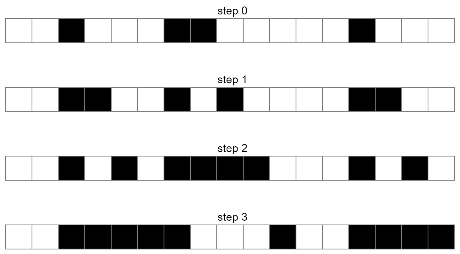
A cellular automaton [1] is a system consisting of cells arranged most often on a one-, two-, or three-dimensional regular lattice, which, at a given instant, are in one of M-th possible states expressing M-valued logic. The dynamics of the model depend on the definition of individual cell states and the rules of transitions between them [2]. One of the simplest examples is a one-dimensional cellular automaton. Suppose that the cells placed on the lattice can be in one of two states, which are marked with white (default assigned to dead state or logical zero) or black color (default assigned to alive state or logical one). We define a rule that if a given cell is black, then the cell to the right of it will change its state. This situation is depicted in a Figure 1. We can observe how the system changes in the subsequent steps of the simulation. The parameter determining the change of the cell state is the state of the left neighbor of a given cell. There are many other possible parameters to choose from—e.g., the condition of the state of both neighboring cells or having nearest neighbors with opposite states. In order to determine the system dynamics, we must have defined the initial cellular automaton states (information about the initial system dynamical state) and a specific set of deterministic or probabilistic rules.

Conway’s Game of Life [3,4] is an example of a cellular automaton with deterministic rules. It was proposed in 1970 by John Conway. The cellular automaton system consists of cells located on a two-dimensional lattice, which can be in one of two states: alive or dead. The rules specify the required number of neighbors and cell states that are taken into account to determine their states in the next cycle (time index). Given the nearest neighborhood of a given cell expressed through the state of 8 closest cells, we can write the 3 main rules of the Classical Conway’s Game of Life (CCGoL) as follows:

1.

If a dead cell has exactly 3 neighbors, it comes alive in the next cycle.

2.

If a living cell has 2 or 3 neighbors, it survives in the next cycle.

3.

If a cell has a different number of neighbors than stated above, it will be dead in the next cycle.

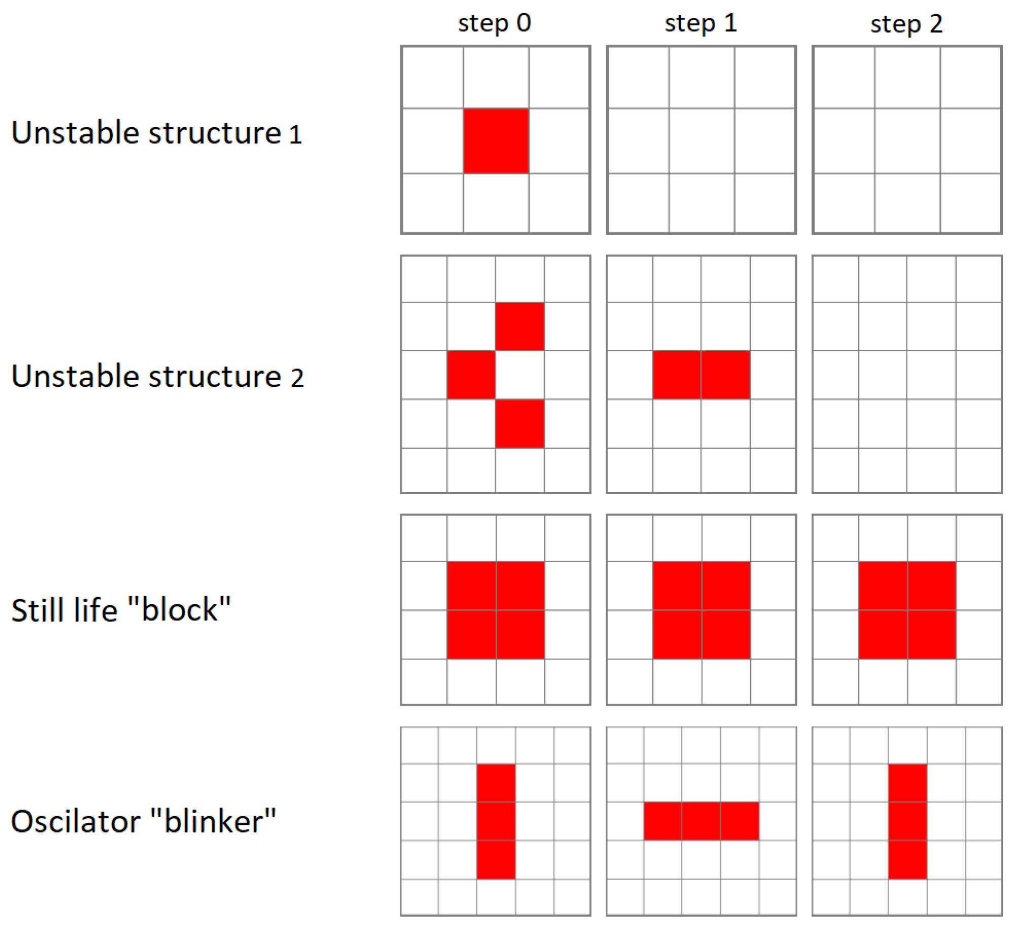
The rules defined in this way allow for the generation of various types of structure topologies with automaton states set to 1, as shown in Figure 2.

The most common type of structures are “unstable structures”, which change in successive cycles but do not return to their initial state. A single cell cannot survive on the lattice because it has fewer than 2 neighbors. A dead cell surrounded by live cells cannot come to life because it has a number of neighbors different from 3. If the simulation is continued for a sufficiently long time, structures usually remain on the lattice that are unchanging over time—“still lifes” (an example is the “block” shown in Figure 2)—or change over time in a periodic way, so they return to their original shape after k cycles—“oscillators” (an example is the “blinker” shown in Figure 2).

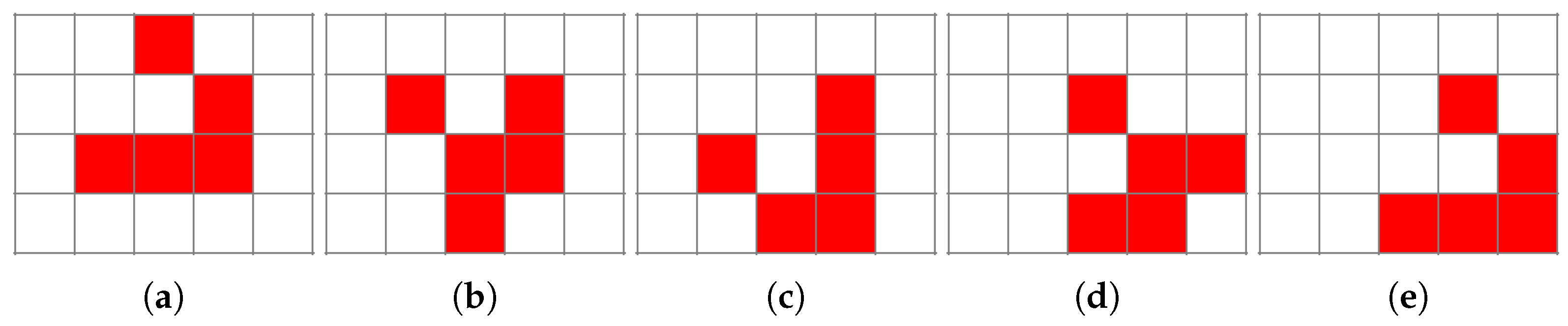
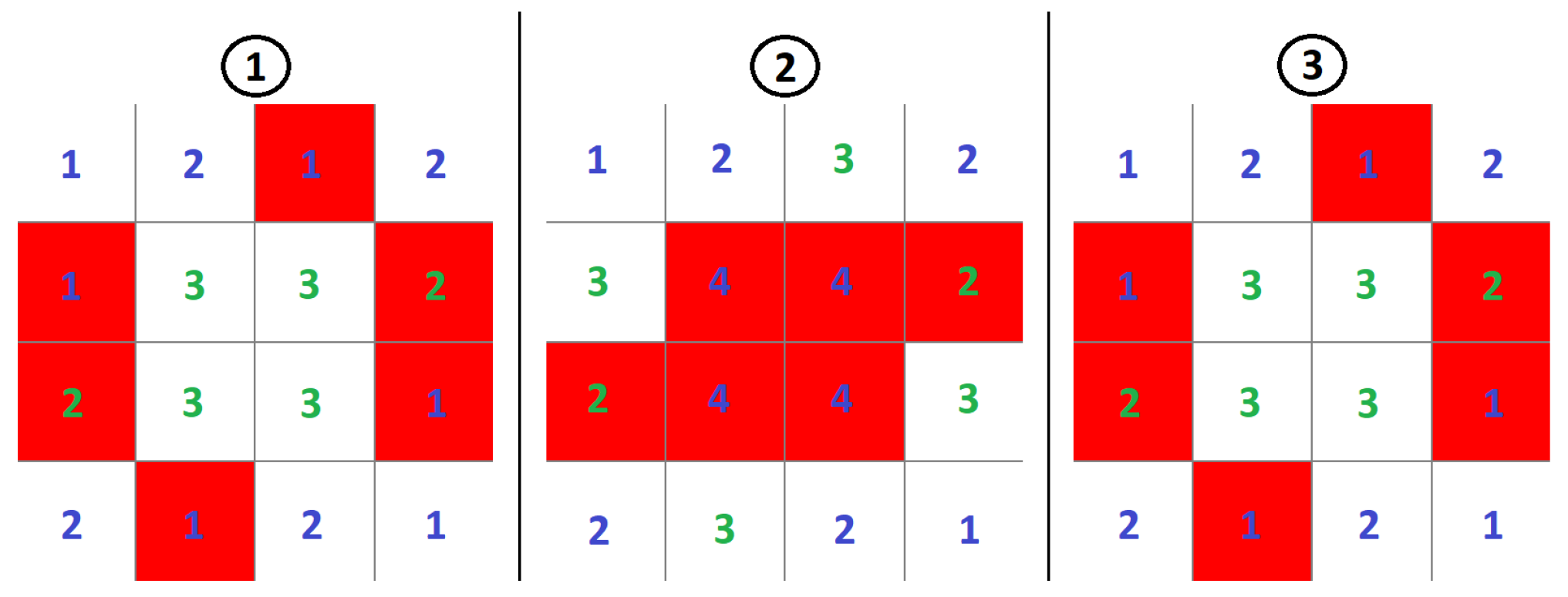
There are also structures that move in a certain direction named “gliders”, as depicted in Figure 3. In a very real way, these gliders behave in accordance with Newton’s first law of dynamics, preserving momentum (speed and direction of propagation in this case). We can also identify “blinkers”, “star ships”, and objects which periodically eject “gliders”—“guns” [5]. Figure 4 shows one of the many oscillators in Conway’s Game of Life during successive iterations of the system simulation.

The “toad” oscillator has a period of 2, which means that it switches continuously between two different fixed configurations. Each 2-dimensional discrete lattice field has a specified number that indicates the number of neighbors of the given cell. If the number is green, the cell will be alive in the next cycle. If the number is blue, the cell will be dead in the next cycle.

2. Introduction to Stochastic Classical Conway’s Game of Life (SCCGoL)

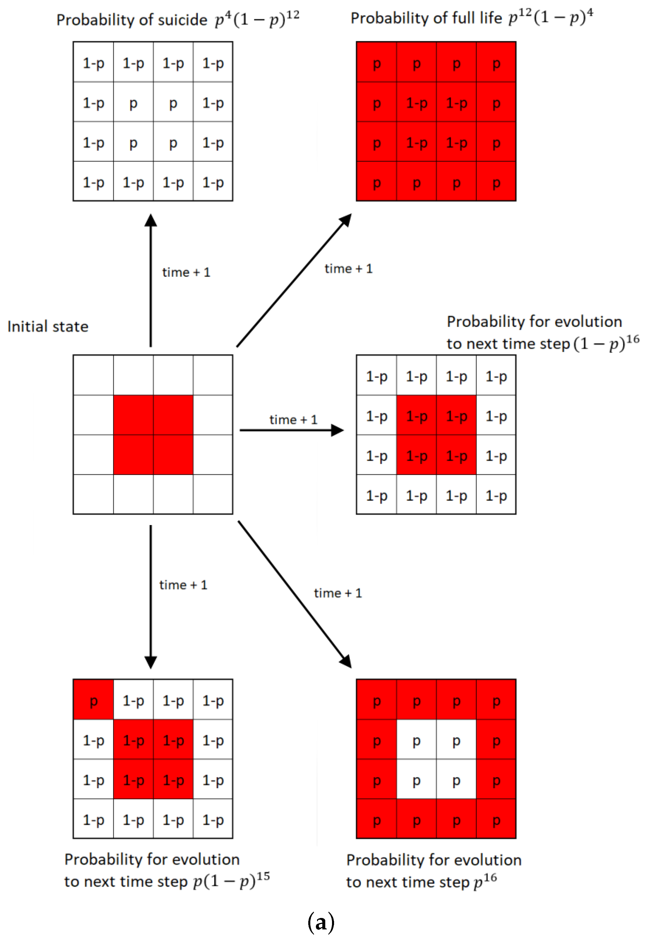
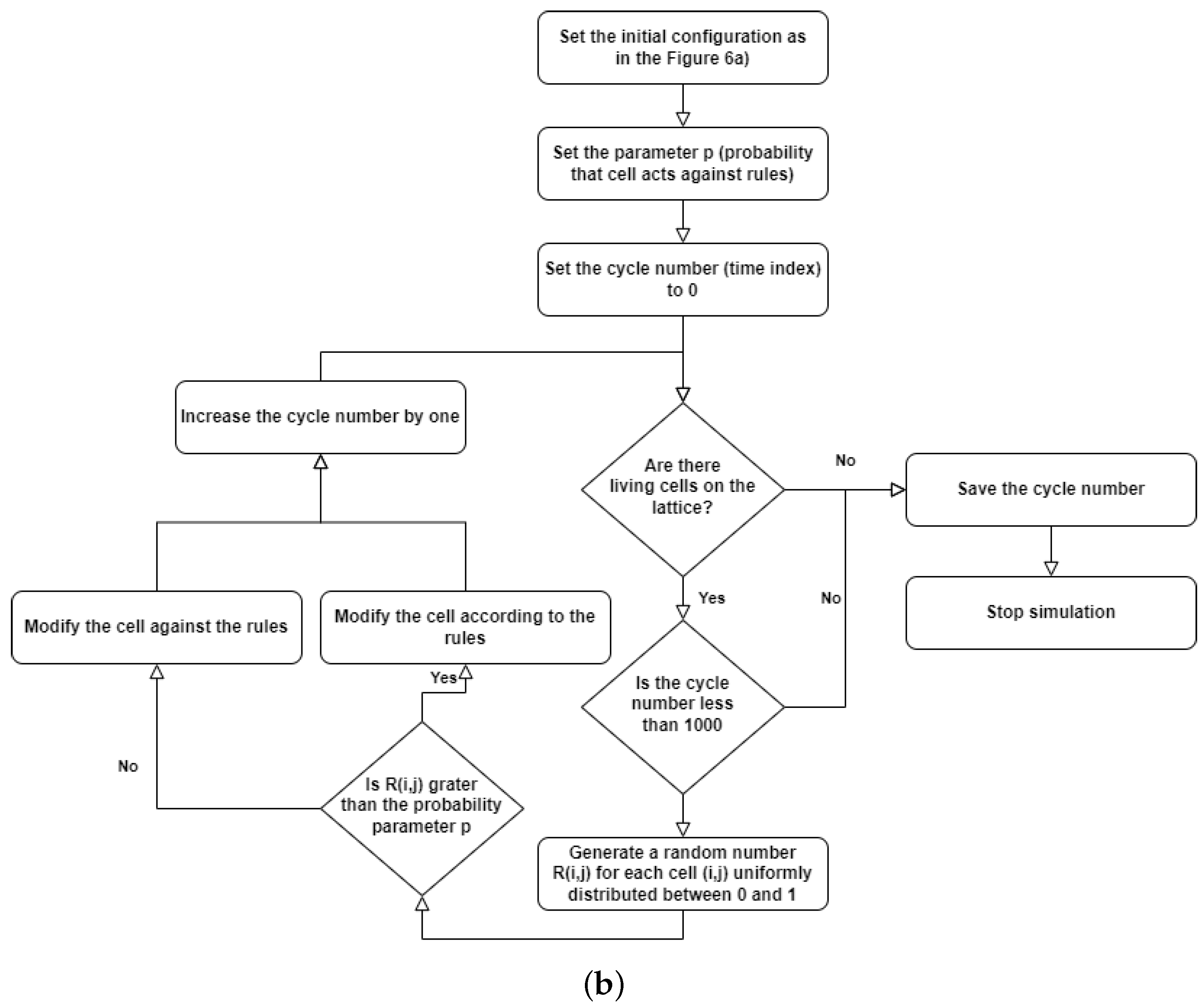
The modification of the fully deterministic Classical Conway’s Game of Life by adding probability to this simulator can be done in a variety of ways [6,7]. The Stochastic Classical Conway’s Game of Life (SCCGoL) was developed from the Deterministic Classical Conway’s Game of Life by adding the probability of spontaneous change to the initially deterministic rules describing the states of cells. With a given prefixed spontaneous probability value p, the state of the cell can change regardless of the number of neighbors resulting only in 0 or 1 (Stochastic Conway’s Game of Life in Discrete mode = SCCGoL(D)). One shall consider all possible scenarios (cell configurations) or subsets of it characterized by a given probability that might take place during the next time step as depicted in Figure 5a. This is somewhat similar to the case of Quantum Mechanics, where one evolves from one point in space to another point in space over a large class of trajectories formally recognized as path integral approach. Instead of discrete values of 0 and 1, we introduce cell states that have continuous values between 0 and 1, which are called mass that will be later assigned to Stochastic Conway’s Game of Life in Continuous mode = SCCGoL(C). Due to the fact that SCCGoLs have different rules from CCGoLs, cells almost never have exactly two or three neighbors. A condition for a given cell to come to life from a dead cell state (creationism of a live cell) is that it has a number of neighbors in a certain range of values. Similar rules apply to a living cell, justifying its live or dead state in the next time iteration. By setting standard intervals of allowed/forbidden numbers of neighboring values, in which the cell is alive/dead, and by adding the additional spontaneous rule probability for the cell to change in the next iteration (probability of changing the state of a cell regardless of the number of neighbors), we are able to create a simulation where the cells almost never die, since it is very difficult from a probabilistic point of view for a given cell to stay alive. If we modify the system dynamics starting from the live cell configuration, it has fixed $1-p$ probability to follow a standard Conway’s Game of Life neighborhood condition for being dead/alive in the already defined intervals during the next time step, and if we select p probability for a cell to change its state during the next time step independently from its neighbors, we can trace various dynamics as we systematically increase the spontaneous probability level p from $0\%$ to $100\%$, resulting in the graph depicted in Figure 6. The algorithm is based on consecutive steps that are shown in Figure 5b.

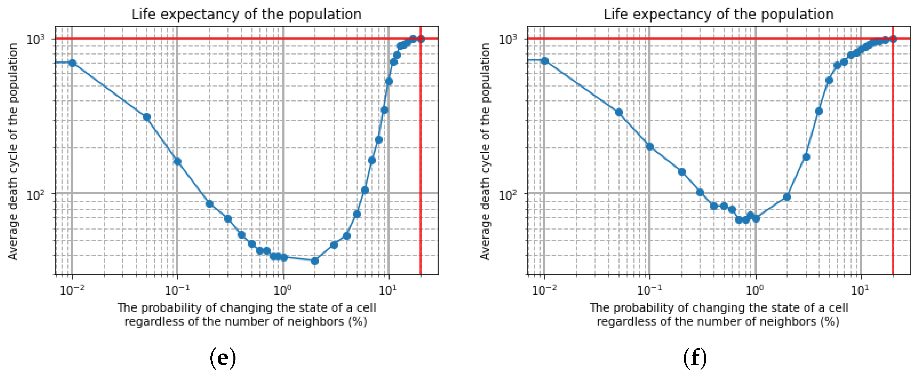
Simulations were conducted for a 10 by 10 and 20 by 20 lattice size with the initial condition of a cellular automaton of 2 by 2 (Figure 6a,b) with the limited maximum number of cycles set to 1000. When the probability of changing the state of a cell p, regardless of the number of neighbors, is equal to zero, there is full determinism; therefore, it is the situation of CCGoL. As the probability increases (in a range from 0 to 2% for a 10 by 10 lattice and from 0 to 2% for a 20 by 20 lattice), the life expectancy of the population decreases due to the lack of neighbors. Starting the simulation from a probability level close to 2% (probability of changing the state of a cell regardless of the number of neighbors), the average life expectancy of the population begins to rise, due to the more frequent appearances of living cells. Conducting the simulation with a probability level above 20%, we observe that the population practically never dies and keeps the average cycle life at least 1000 time iterations.

3. Generalization of Stochastic Classical Conway’s Game of Life (SCCGoL) to the Case of $\mathit{N}$ Competing Cellular Automaton Species

The created simulation platform enables the creation of N different cellular automaton species that compete between themselves for the resources needed to replicate. A given automaton species has better replication properties within its own community and worse replication properties when its neighbors are of a different species. Such a situation is normally encountered in human populations, where people of one homogenous identity prefer to collaborate together rather than with people with a very different identity (from a different tribe). Therefore, a soft antagonistic relation between different species is introduced indirectly by means of a higher level of tolerance (or effectiveness of replication) towards neighbors of the same species than for neighbors of another species (other different species are treated in the same way). In a real way, this is analogous to how members of a given nation or culture collaborate within a given culture or community, as opposed to a different culture or community. Let us consider $N=4$ (number of different automaton species), so we have the following determined formula for the number of effective existing neighbors ${\widehat{N}}_{effective,k}$ for given k-th tribes:

$${\widehat{N}}_{effective,k}=a_{1,k}{\widehat{N}}_1+a_{2,k}{\widehat{N}}_2+\cdots +a_{k,k}{\widehat{N}}_k+\cdots +a_{k,N}{\widehat{N}}_N.$$

(1)

The previously defined replication rules promoting a given cell’s own species (preference of own tribe) can be formally expressed by the condition (max($a_{s,k})=a_{k,k}$ and $a_{k,k}>a_{s,k}$ if $s\ne k$). In the conducted simulations, all tribes have assigned the same value ($a_{1,1}=a_{2,2}=a_{3,3}=a_{4,4}=\frac{1}{2}$) and another same value for ($a_{1,2}=a_{1,3}=a_{1,4}=a_{2,1}=a_{2,3}=a_{2,4}=a_{3,1}=a_{3,2}=a_{3,4}=a_{4,1}=a_{4,2}=a_{4,3}=\frac{1}{3}$), which simply means that automaton tribes promote their own tribe and only partly promote other tribes, with no special distinction regarding which different tribe it is pointing to. The cellular automaton species distribution for the k-th tribe across a two-dimensional lattice is generated with use of a two-dimensional Gaussian distribution, as follows:

$$f{(x,y)}_k=A_k{e}^{-\left(\frac{{(x-x_{0,k})}^2}{2{\sigma }_{x,k}^2}+\frac{{(y-y_{0,k})}^2}{2{\sigma }_{y,k}^2}\right)},$$

(2)

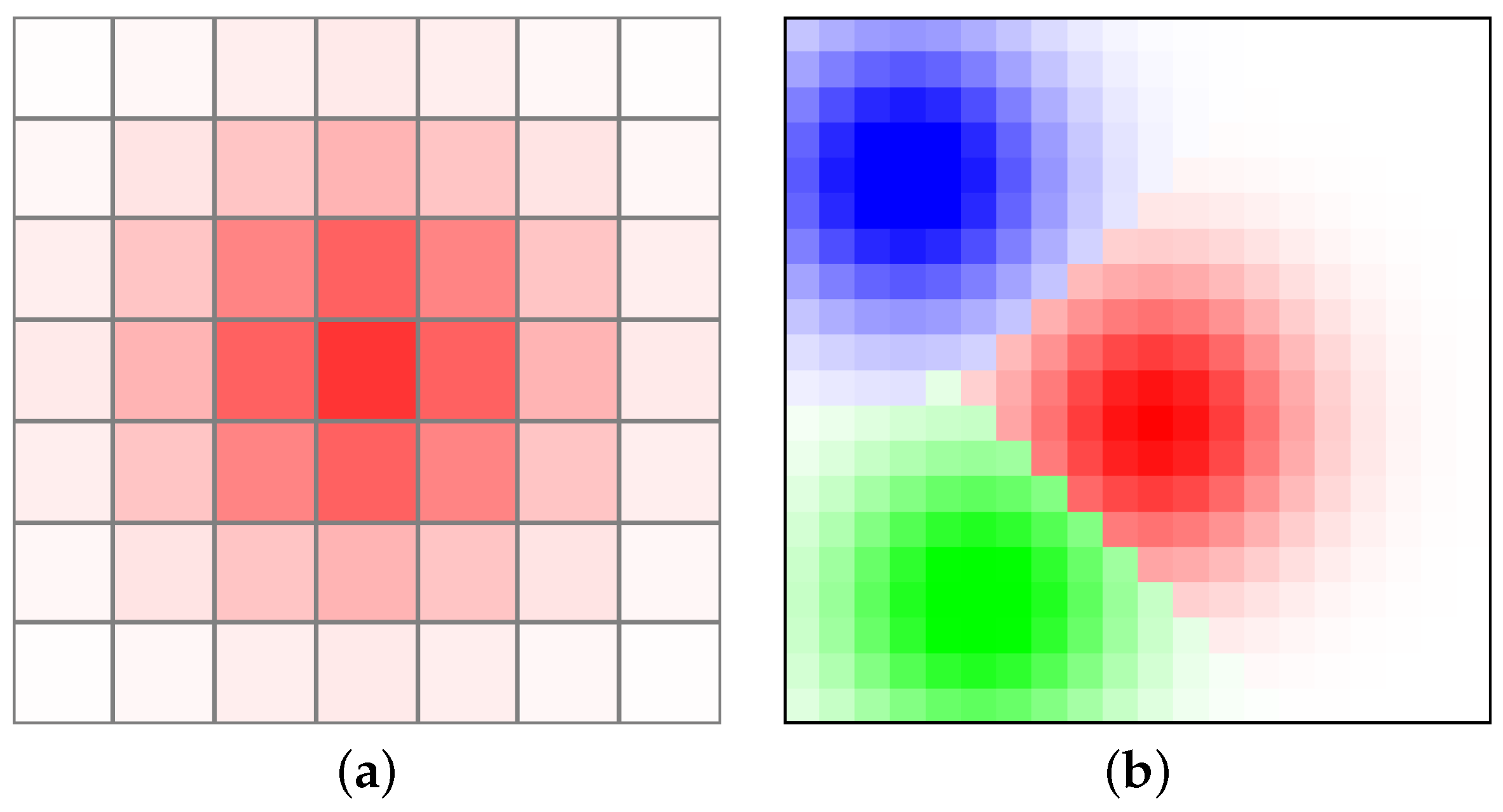
where $f{(x,y)}_k$ is a mass function depending on the cell coordinates and $(x_{0,k};y_{0,k})$ is the center of the given cellular automaton species. Given parameters $A_{0,k}$ and ${\sigma }_{x,k}$, ${\sigma }_{y,k}$ can control the mass of species and spread across the “Globe”, as depicted in Figure 7.

In the case of several species on the lattice, SCCGoL simulation results promote the formation of new cells among the species that has the most mass in the neighborhood, as illustrated in Figure 8. During the life cycle, a newly formed cell always has a mass that is more dependent on cells of the same species than on another species of neighbor. We observed that automata species fight each other to spread across the lattice and exclude other species, which is an expression of some form of biological Darwinism, as a consequence of Formula (1).

4. Methodology of Describing SCCGoL Dynamics Using Tools of Classical Statistical Physics

Adding probability to the initially deterministic Game of Life and changing the interaction rules between neighboring automata required the introduction of a new quantity called mass with continuous real values (other than 0 and 1 present in the deterministic Game of Life). At this stage, the aliveness of the whole cellular automaton population can be understood and approximated by the total energy of the population (where mass is simply equal to energy). The level of the automaton distribution order is expressed by the entropy. Entropy was introduced by Rudolf Clausius in 1865 as a thermodynamic state function [8,9]. If the entropy in the initial state and the entropy of the final state are denoted by $S_i$ and $S_f$, respectively, then we have:

$$S_f-S_i={\int }_i^f\frac{dE}{T},\frac{dS}{dE}=\frac{1}{T}$$

(3)

The very last formula gives a definition of temperature, under the assumption that energy and entropy are defined. Instead of thermodynamic entropy, we use the Shannon entropy measure, given as:

$$S_{Shannon}=-\sum _{i,j}p(x_i,y_j)logp(x_i,y_j)=\mathbb{E}\left[-logp(x,y)\right]$$

(4)

In order to calculate the probability in the Equation (4), the SCCGoL simulation is repeated several hundred times, giving an average population cell mass in successive cycles.

The temperature, which is a measure of thermal state, was calculated using Equation (3) in a changed form:

$$T(x,y,t)=\frac{\frac{dE(x,y,t)}{dt}}{\frac{d{S}_{Shannon}(x,y,t)}{dt}}=\frac{dE(x,y,t)}{d{S}_{Shannon}(x,y,t)}$$

(5)

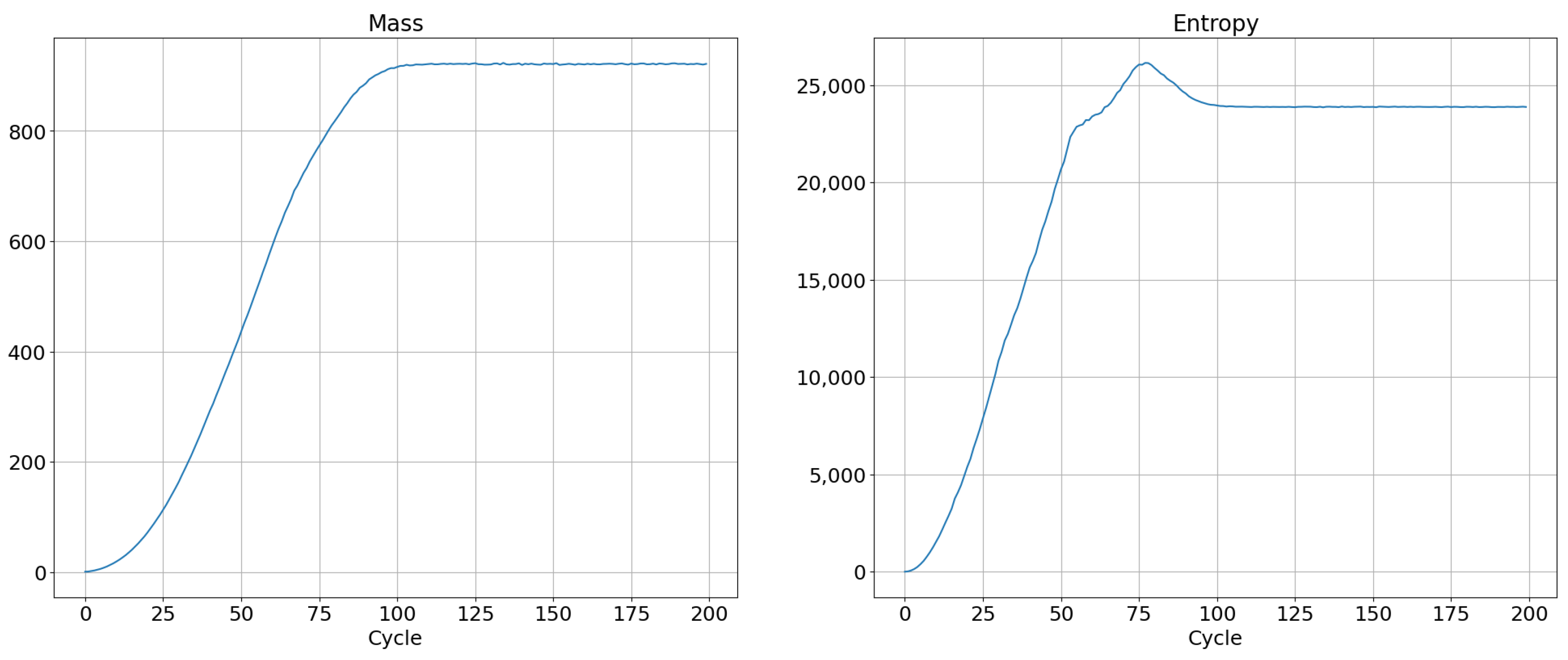
The temperature defined by this formula can be calculated by two different methods. The first method relies on calculation of the energy and entropy for the entire system, followed by numerical calculation of the derivative of energy with respect to the function of entropy. The second approach is to differentiate mass and entropy with respect to simulation time for each cell. As a result of the corresponding ratio, we obtain a temperature map. An example of the evolution of mass and entropy for SCCGoL is depicted in Figure 9. It shows maximization and saturation of entropy, which is in accordance with the Second Law of Thermodynamics in physical systems, although we are dealing with a cellular automaton system. On the other hand, the mass of a system saturates and increases to a certain critical value, as shown in the left side of Figure 9.

5. Numerical Analysis of SCCGoL Dynamics with Methodology of Classical Statistical Physics

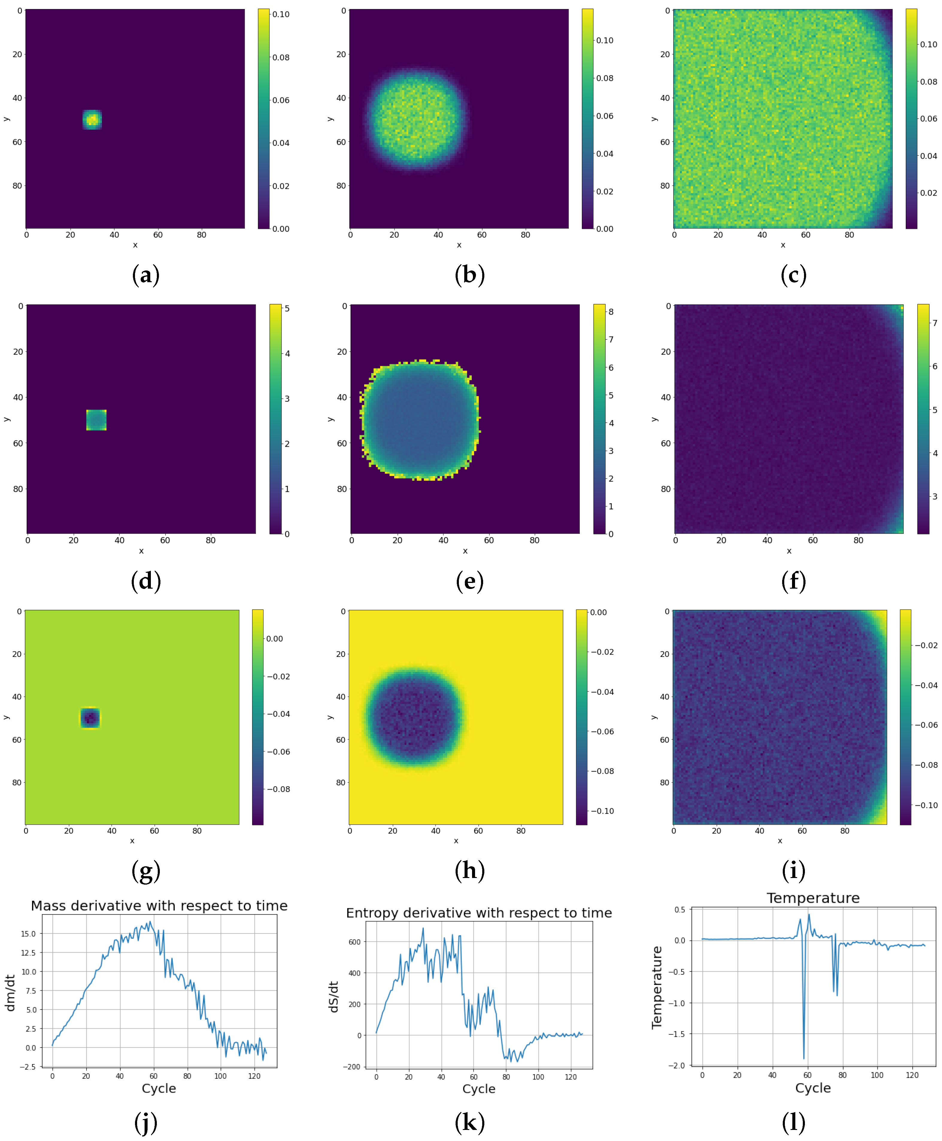
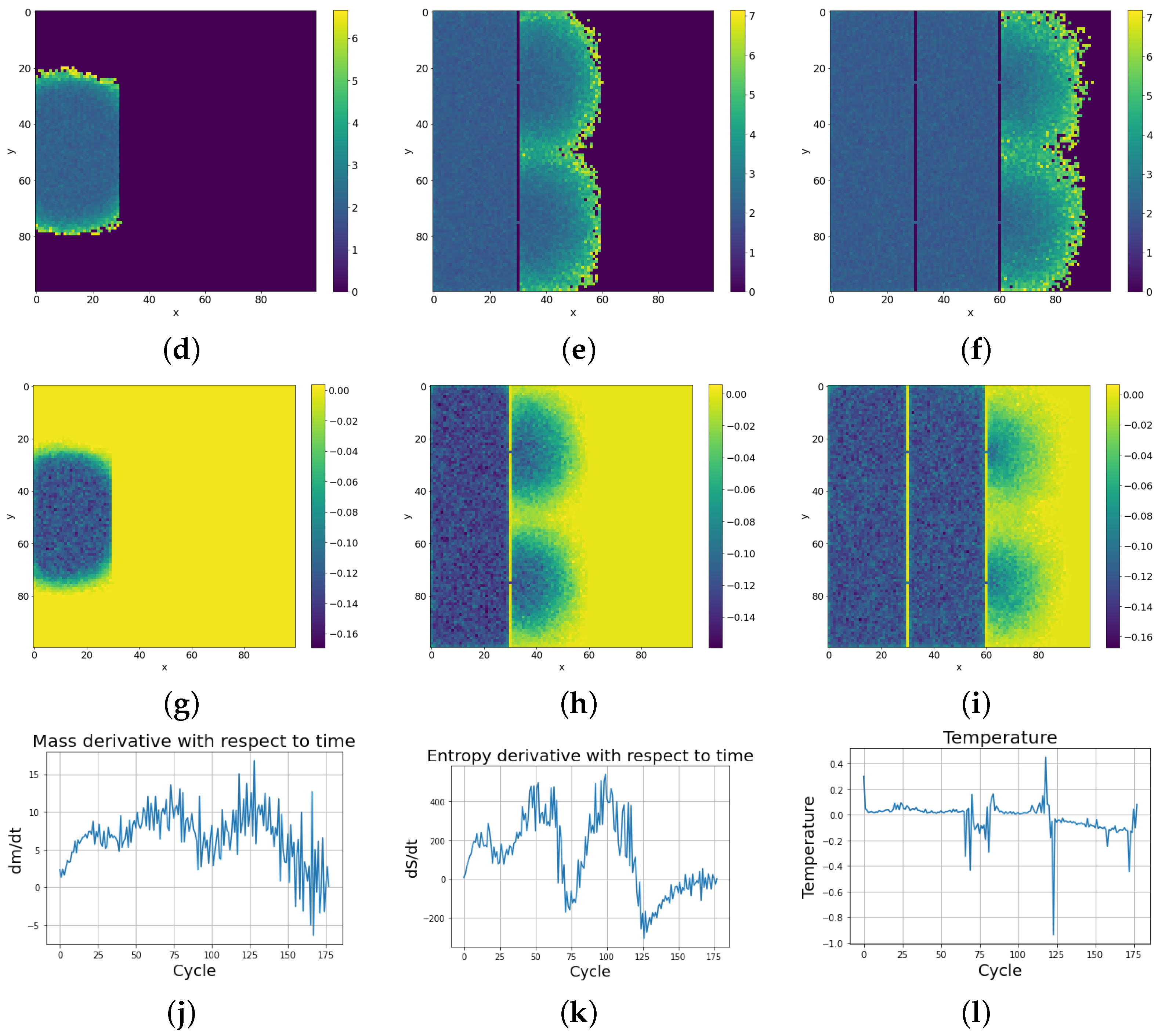
Numerical simulations were carried out for four topologies of cellular automata. We preimpose a rule that a given live cell has 20% probability of changing its state to a dead state and that an initially dead cell has a 20% probability of changing its state to a live state, with a mass chosen randomly from uniform probability density from an interval value of 0–0.5. The state of a given cell is still dependent on its neighbors, since it has 80% probability of changing its state due to the state of its neighbors. In order to obtain the probability distribution dependence on time, during simulations the frequency of positions of the cellular automata across a 2-dimensional lattice were determined. Figure 10a shows a lattice of size 100 by 100 with one cell alive as the initial lattice state for which various thermodynamic parameters were obtained (depicted in Figure 11).

Figure 10. (a,b) Evolution of diffusion process in cellular automaton system for a limited lattice size of 100 by 100 in SCCGoL(C) (averaged over 1000 trials). The final saturation of mass and entropy (as depicted in Figure 9) implies values approaching thermodynamic equilibrium with characteristic fluctuations of mass and entropy around effective stationary values.

Figure 10. (a,b) Evolution of diffusion process in cellular automaton system for a limited lattice size of 100 by 100 in SCCGoL(C) (averaged over 1000 trials). The final saturation of mass and entropy (as depicted in Figure 9) implies values approaching thermodynamic equilibrium with characteristic fluctuations of mass and entropy around effective stationary values.

With subsequent cycles, the cells occupy more and more space on the lattice, which can be seen as increases in the mass of the entire system (possible mass creationism is an inherent feature of Conway’s Game of Life). The sum of the masses of all cells in successive cycles is depicted in Figure 9 with a comparison of the entropy change of the entire system. As can be seen in Figure 11e, high entropy occurs at the edges of the population, which is caused by the entropy wave meeting the area with almost zero cell occurrence. Before equilibrium is established, the entropy of the system slightly decreases, due to the loss of this extra entropy at the edges, as can be seen on the right side of Figure 9. Having established these two quantities, we differentiate them with respect to time, and using Formula (3) establish the whole effective temperature of the system by dividing the change of mass at a given time by the change of entropy. Figure 11k shows the greater susceptibility of the entropy change to the constraints associated with the limited size of the simulation lattice, which is ended with impenetrable walls. The dependence of mass derivative with respect to time simulation (Figure 11j) does not have such large oscillations as in the case of the entropy derivative with simulation time (Figure 11k). The temperature calculated by this procedure gives values just above zero (slightly positive) up to the 50th cycle. We can see a large down peak caused by a slowdown in entropy increase. From about the 75th cycle, the temperature of the system goes from positive to negative values. Figure 11l) shows the anomalous thermalization process in SCCGoL, approaching temperature and entropy equilibrium. Surprisingly, thermodynamic equilibrium is achieved in the case of negative temperatures. A second possible approach to determine the temperature is by using the derivatives of the mass and entropy of the individual cells with respect to time and obtaining a temperature map of all the cells. The temperature depicted in Figure 11i is mostly negative and steady, which corresponds to a situation where mass and entropy have come to equilibrium. We can distinguish two regions in the simulation. The first has no temperature gradient and zero negative temperature. The second region has a non-zero temperature gradient that also includes positive temperatures. The time derivatives of mass and entropy have noticeable values at the edges of the automaton population, where we observe a slightly positive temperature, which corresponds to the situation in Figure 11l before the 75th cycle.

6. Numerical Study of One-Species Cellular Automata with Various Boundary Conditions

The next family of simulations were conducted using barriers impenetrable to cellular automaton cells, so the cellular automata cannot cross the barrier or interact via barrier.

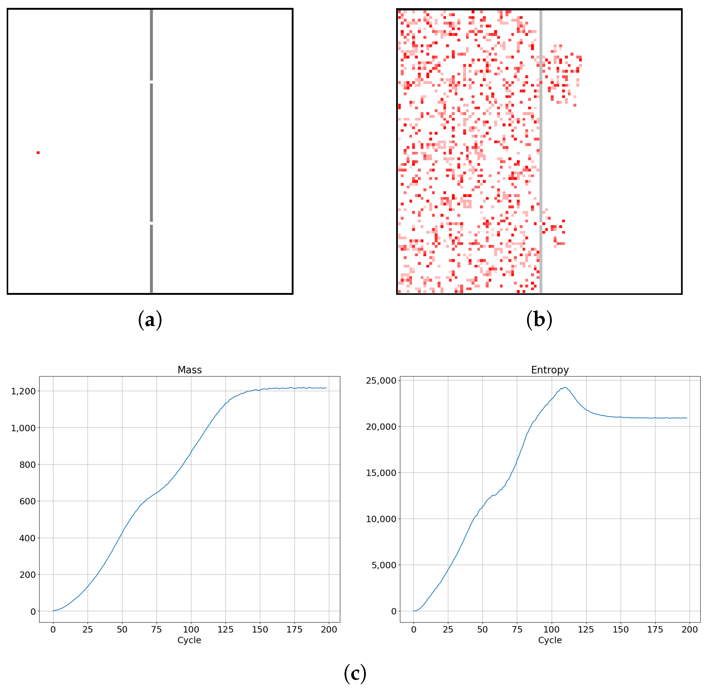
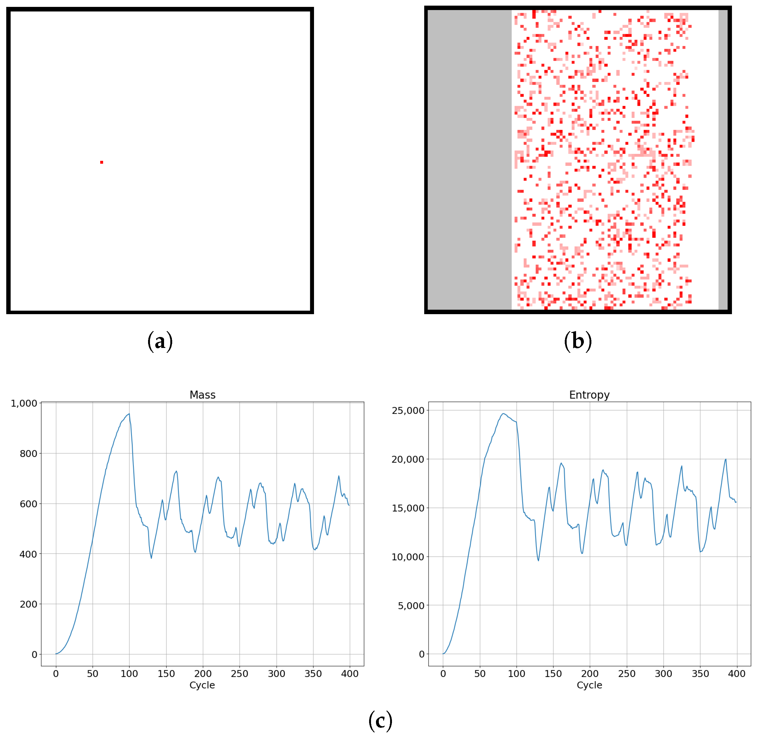
Let us consider a single cellular automaton (single automaton seed) placed in an empty chamber with impenetrable walls, linked by two small holes to another empty chamber, as depicted in Figure 12a. We observe a diffusion of cellular automata with simulation time, consisting of two main processes: the creation and diffusion of cellular automata in the first chamber and diffusion of cellular automata from the first chamber into the second chamber, accompanied with the creation of new automata in the second chamber. These two consecutive processes are accompanied by an effective slowdown in diffusion, as can be seen on the left in Figure 12c. At the same time, we can observe a slowdown in entropy increase, as shown on the right side in Figure 12c. Once mass saturation was obtained in the simulation, we observe maximization and a small drop in entropy that later stabilizes and saturates, as seen on the right in Figure 12c.

Entropy, unlike mass, is characterized by a large variation in the values in the middle of the population and at the edges of the cellular automaton population. In the situation with a barrier (Figure 13e), this is particularly evident after the cells pass through the gaps. This particular process is due to the logarithm function dependence of Von Neumann entropy, which tends to negative infinity for arguments going to zero from the right. The observed criterion for equilibrium is the fact that mass and entropy have steady values and that temperature has a negative value in thermodynamic equilibrium. Almost always before the equilibrium moment is achieved, time derivatives of mass and entropy have positive values, and the temperature is still positive. From the moment equilibrium is achieved, we observe small fluctuations of entropy and temperature. A slight increase in mass results in a slight decrease in entropy and vice versa. Analogously to the system with one barrier, simulations were conducted on the system with two barriers and the initial structure depicted in Figure 14a.

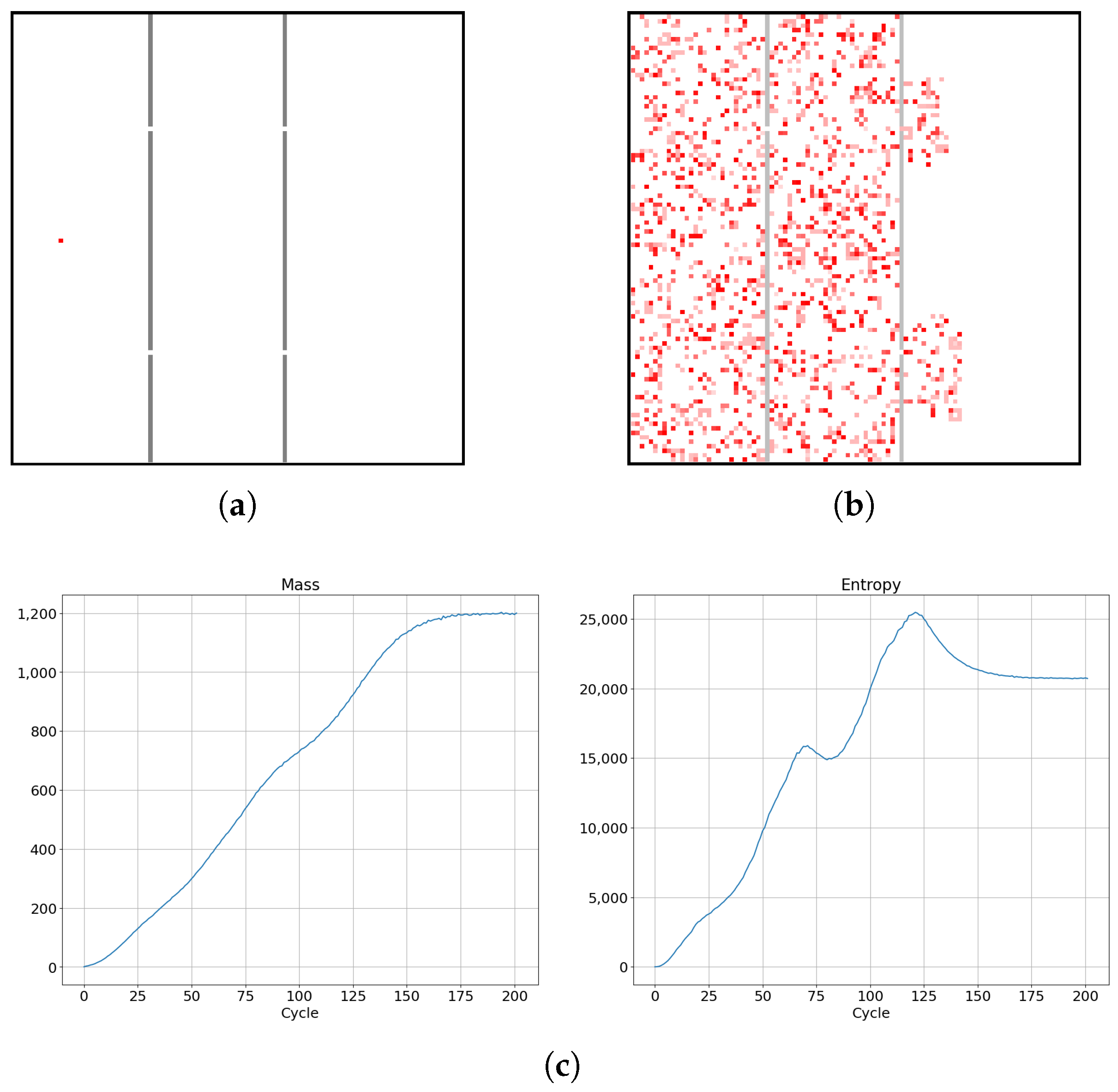
Let us now consider a single cellular automaton placed in an empty chamber with impenetrable walls and two small holes linking it to a second empty chamber, which is connected to a third empty chamber by impenetrable walls with two small holes, as depicted in Figure 14a. We observe the diffusion of the cellular automaton with simulation time, corresponding to three main processes: creation and diffusion of the cellular automaton in the first chamber; diffusion of the cellular automaton from the first chamber into the second chamber, accompanied with the creation of new automata in the second chamber; diffusion of cellular automata from the second chamber into the third chamber, accompanied with the creation of new automata in the third chamber. Two observed local peaks in the entropy increase reflect the situation where the cells try to reach the impenetrable barriers and, quite soon after, entropy drops. After the occurrence of the second entropy peak, entropy drops and later stabilizes and saturates, as shown on the right in Figure 14c.

It takes longer for mass and entropy to reach equilibrium in a system with two barriers than in the case of a system with only one barrier. As depicted in Figure 15k, due to the cells approaching the barriers and losing the extra entropy at the edges of the population, we observe significant fluctuations in the time derivative of the entropy. This results in large peaks, as can be seen in Figure 15l.

7. Numerical Study of Two-Species Cellular Automata in Perturbative Interaction by Narrow Constriction

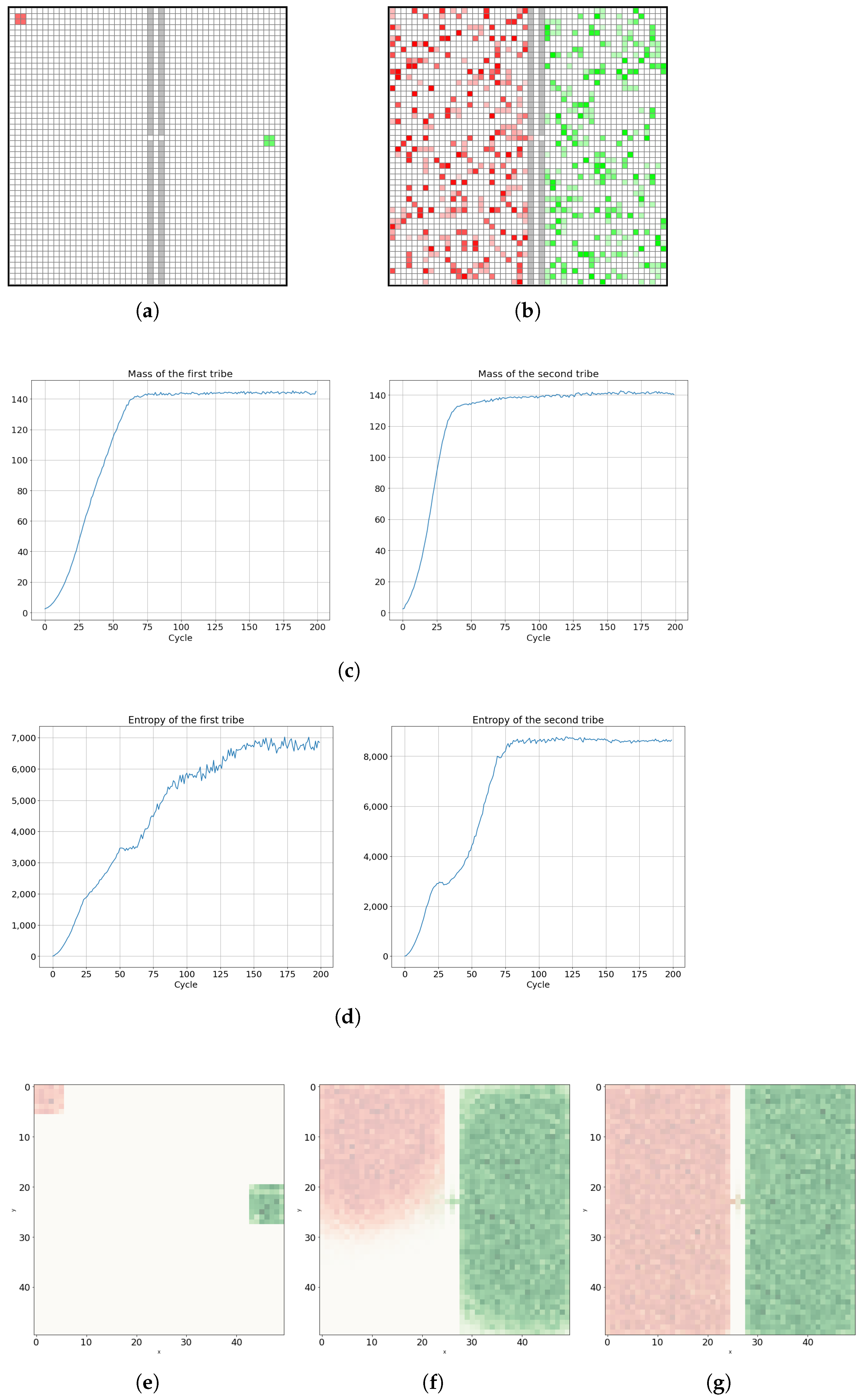
Further simulations for the case of two species cellular automata were carried out for a system divided into two reservoirs separated by two impenetrable barriers with one small hole (Figure 16a), implying perturbative interaction between tribes.

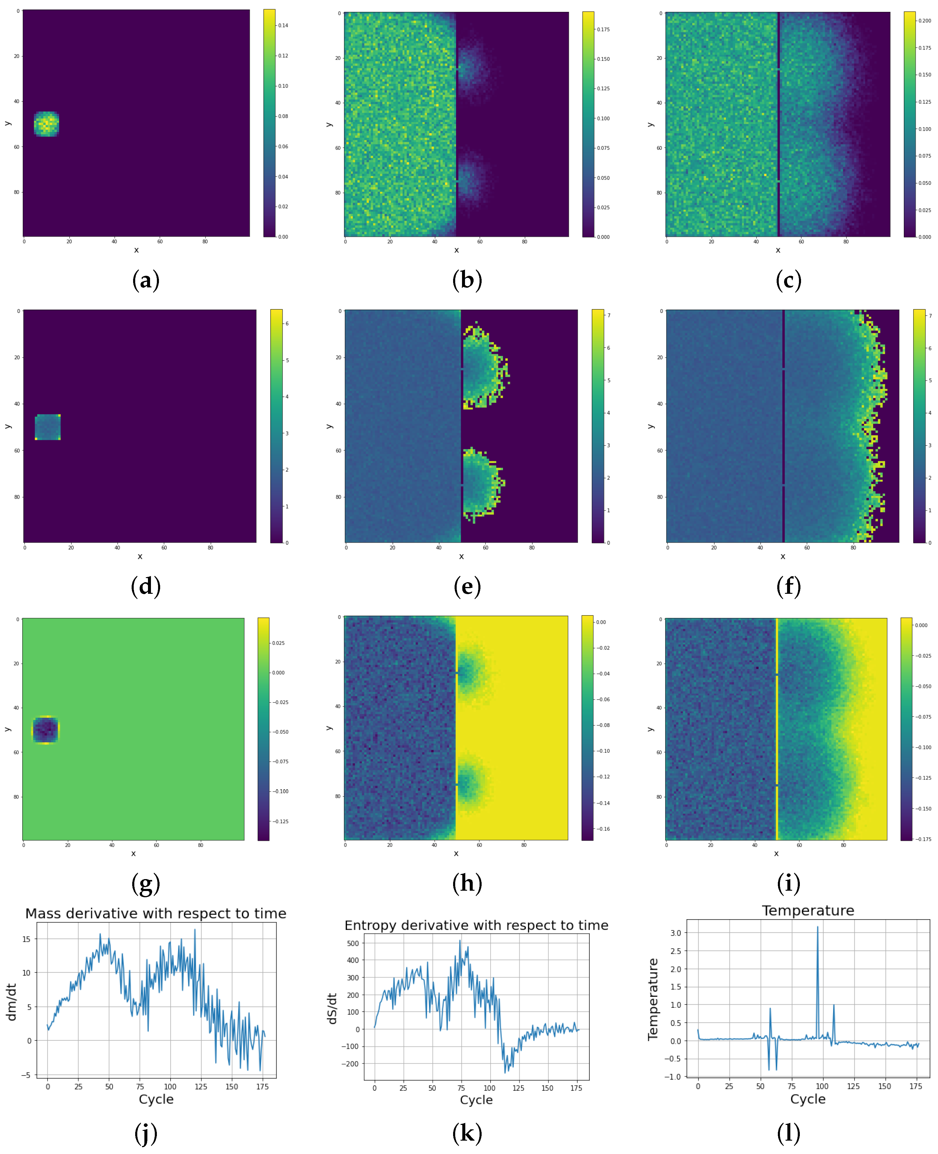
In the left upper corner of the first part of the system, there are located cells of the first cellular automaton tribe. At a closer distance to the hole in the impenetrable wall, but in the second right reservoir, there are located cells of the second cellular automaton tribe. In Figure 16c, we can observe similar final masses and their dynamics for both tribes, but Figure 16d shows different entropy dynamics. The effect of different entropy dynamics among two tribes is due to the initial distance of the cellular automaton tribes from the small hole in the impenetrable wall. A tribe located further from that hole needs more time to propagate and occupy its natural neighborhood and the first left chamber of the system, and thus this tribe has a lower probability of taking over the territory of the other tribe. However, the mass and entropy of both tribes achieve equilibrium and finally the tribes end up in a similar geometrical and dynamical situation. As depicted in Figure 16f, the tribe on the right side, closer to the small hole in the barrier, occupies the territory of its nearest neighborhood more quickly, resulting in the later attempt to occupy the territory of the rival tribe that can only be achieved by diffusion via small hole.

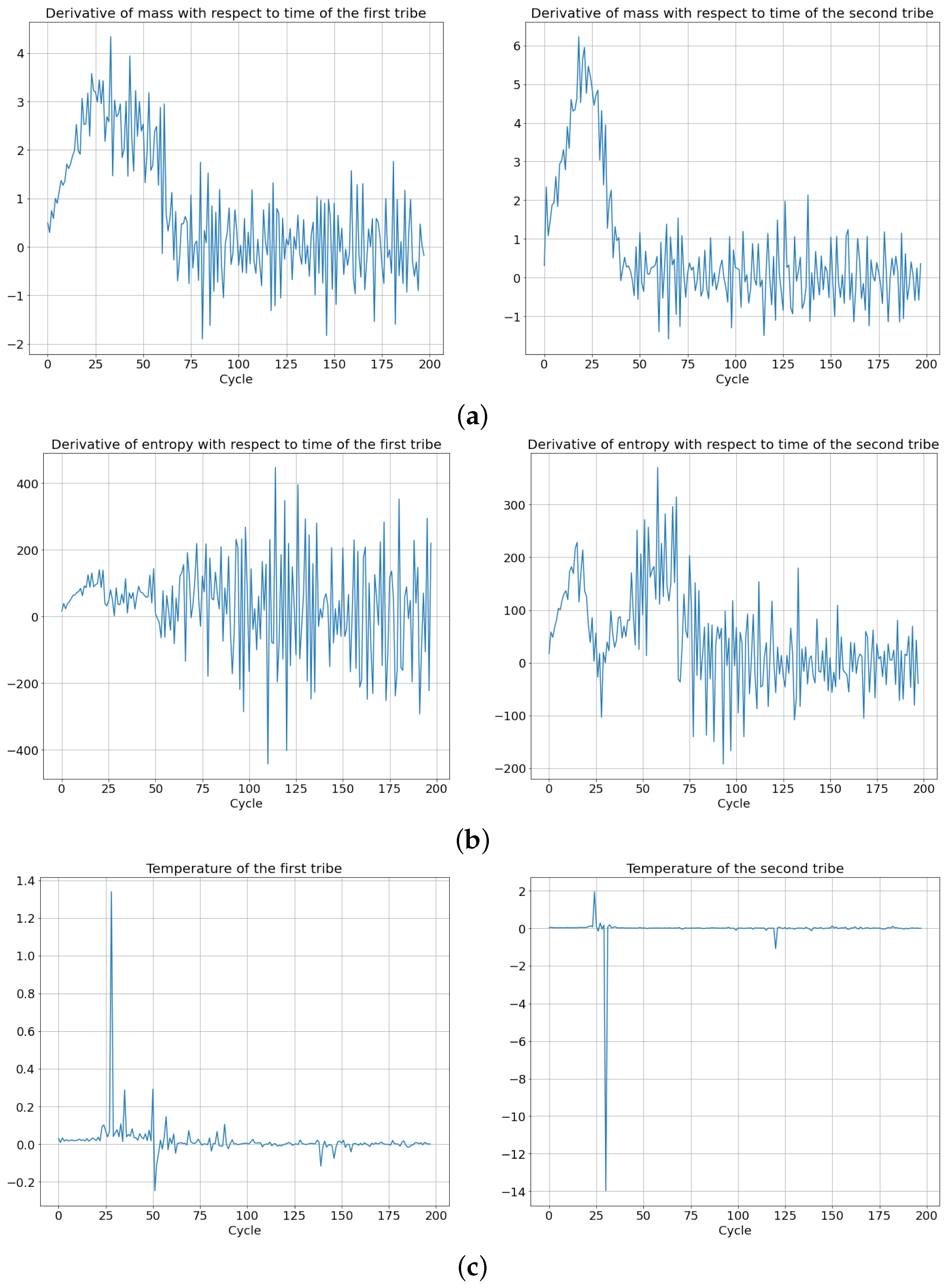
As depicted in Figure 17, large oscillations were observed in the time derivatives of mass and entropy of both cellular automaton tribes. In contrast to the previous simulations, the temperature of the system after reaching equilibrium was not characterized by a negative value only. Existential competition between tribes resulted in both positive and negative temperatures.

8. Behavior of One-Species Cellular Automata with Cycle Movement of Barriers Mimicking Thermodynamical Cycle

In SCCGoL, it is possible to control the mass and entropy of a cell population in a dynamical way in a cyclic or not cyclic way by adding moving barriers to the system. The next simulations were conducted on a lattice size of 100 by 100 and with two barriers expanding and shrinking sinusoidally starting from the 100th cycle. The first one moves from the left edge of the lattice to the right with an amplitude equal to 30 space lattice and a period of 20 cycles (time indices), and the second moves from the right edge of the lattice to the left with an amplitude equal to 30 space lattice points and a period of 57 cycles (time indices). The initial structure of the simulation along with the fragment of the simulation with visible barriers are shown in the Figure 18.

As shown in Figure 18c, the mass and entropy of the system for the first 100 cycles increases as the cells spread across the lattice. Then the left and right barriers start to move towards the center; thus, the cells are suppressed by the contraction of their chamber volume. In the graph, this is represented by a drop in mass and entropy. The left barrier begins to move back after 10 cycles, and the right one after 29 cycles, giving the opportunity to reoccupy the lattice by cells in case of chamber volume expansion. This process is repeated in successive simulation cycles.

As depicted in Figure 19, we are able to effectively reduce the mass and entropy of the system by using movable barriers. The result is a quasi-periodic behavior of the system. This does not apply to temperature, which remains positive due to the fact that the mass and entropy do not reach equilibrium. This property (positive temperature) characterizes the system with moving barriers in SCCGoL. As can be seen in Figure 19c, as the barrier moves away from the center of the lattice, the entropy of the newly formed cells is higher than that of the cells in the center. On the other hand, the approach of the barrier to the center of the lattice results in a greater mass of cells at the edge of the population, which is caused by pushing the cells from neighboring fields, which can be seen in the temperature graph in Figure 19h.

9. Conclusions and Future Perspectives

Cellular automata can simulate many complex physical phenomena using simple rules, while still being an effective approximation. In this study, we have presented the diffusion dynamics of cellular automata, given by various simulations for one and many automaton species. In most cases, we observe linear diffusion in two dimensions with some non-linear components that can be encapsulated by the mathematical structure known as the second Fick’s law given as $\frac{\partial p}{\partial t}=D(x,y,t,p)(\frac{{\partial }^{2}p}{\partial x^2}+\frac{{\partial }^{2}p}{\partial y^2})$, where $p=p(x,y,t)$ can be assigned to values of cell vividness on a two-dimensional lattice (mass value). It should be underlined that the existence of non-linear diffusion is due to the fact that the $D(x,y,t,p)$ is non-constant in time and space, while in the case of lack of dependence of D on $(x,y,t,p)$, we are dealing with linear diffusion. Similarly as in the case of mass distribution of cells in two dimensions, we can trace temperature and entropy diffusion that can be correspondingly assigned to different coefficients $D_1$ and $D_2$, which can also depend on $(x,y,t,T)$ or $(x,y,t,S)$. Clearly witnessed diffusion across various physical quantities, such as mass distribution, temperature and entropy, is quite a prominent observational feature that also occurs in hydrodynamics or in condensed matter systems. Yet, we are dealing here with features of programmable matter, as we set rules of interactions of automata in accordance to predefined schemes, that can be time independent or time dependent or even position dependent. Furthermore, we are able to mimic cycle thermodynamic processes, which shall draw the attention of experts in statistical physics. Usage of the methodology of statistical physics applied to cellular automata dynamics always has to do with an oversimplified picture that omits microscopic automata degrees of freedom, as is expressed by the D coefficient. The dynamics of four automaton species showed quasi-Darwinist competition (Figure 8). Despite the fact that the principle of conservation of mass is not fulfilled, since we have creationism and annihilation of automata, the SCCGoL dynamics provide strong evidence that the entropy and temperature attain equilibrium. In various simulations of the Stochastic Conway’s Game of Life dynamics, we observed a transition from positive to negative temperature values. A maximum level of mass and energy density was reported among cellular automata, since otherwise they would die due to overpopulation. The fact that temperature can be negative is known from condensed matter physics, but with the assumption that the energy is top-bounded. In most “normal” situations this is impossible, but in rare cases in solid state physics it can be achieved approximately by inverting the population state. Obviously, there is also such a limitation on the top-bounded energy value (mass density value) in the Stochastic Conway’s Game of Life. Therefore, it is consistent with the laws of thermodynamics, as pointed out by Prof. Adam Bednorz (Faculty of Physics, University of Warsaw).

The following contributions were derived based on our simulations and the described methodology:

1.

Identification of thermodynamically defined temperature as a proper measure of system evolution with a ‘minus’ sign for a system with mass and entropy in equilibrium (Figure 11, Figure 13 and Figure 15).

2.

Identification of mass as the effective energy of the system (in first approximation) (Figure 9, Figure 12, Figure 14 and Figure 16).

3.

Identification of Shannon Entropy as effective system entropy (in first approximation) (Figure 9, Figure 12, Figure 14 and Figure 16).

4.

Generalization of Stochastic Conway’s Game of Life for N tribes (approximated analogy to N-body Quantum Physics can be conceptually drawn) as depicted in Figure 8 and Figure 16.

5.

Confirmation of the validity of the second law of thermodynamics in SCCGoL (entropy maximises and saturates, Figure 9, Figure 12 and Figure 14).

6.

Identification of a brief Shannon entropy peak that later minimizes and saturates in SGoL (Figure 9 and Figure 12). Monotonicity in increase of entropy is twice briefly interrupted by a small decline, which is associated with automaton cells “colliding” with the barriers and experiencing a brief propagation slowdown (Figure 14).

Our analysis of the Stochastic Game of Life allows such systems to be treated as mathematical objects well described by the methodology of classical statistical physics. The numerical results obtained by various simulations suggest that another definition of temperature can be introduced in the Stochastic Conway’s Game of Life system by adding a ‘minus’ sign to temperature, known in statistical physics, so we obtain the following formula:

$$Temperatur{e}_{Conway-Pomorski-Kotula}=-\frac{dE}{dS}$$

(6)

$$Temperatur{e}_{StatisticalPhysics}=+\frac{dE}{dS}$$

With this definition of Conway-Pomorski-Kotula temperature, we can use the tools of statistical physics in the Stochastic Game of Life, preserving most intuitions from classical thermodynamics concerning various situations we may encounter. There are well-known inherent analogies between classical statistical physics [10,11,12,13,14] and quantum mechanics [15,16]. Therefore, further research perspectives in the study of Stochastic Classical Conway’s Game of Life assume the use of quantum mechanics to simulate classical statistical physics (as expressed by the epidemic model or stochastic finite-state machine), as explicitly represented by the tight-binding model [17,18] or Schroedinger model, directly proposing structures implemented in semiconductor single-electron devices. The obtained probability map of the Stochastic Conway’s Game of Life has relatively non-rapid changes of mass distribution over space and should be parameterized using a non-linear Schroedinger equation and, especially, by using the Ginzburg-Landau model [19]. This could be the basis for the quantization procedure of the Stochastic Classical Conway’s Game of Life [20].

References

- Berto, F.; Tagliabue, J. Cellular Automata. In The Stanford Encyclopedia of Philosophy, Spring 2022 ed.; Zalta, E.N., Ed.; Metaphysics Research Lab, Stanford University: Stanford, CA, USA, 2022. [Google Scholar]
- Wolfram, S. Statistical mechanics of cellular automata. Rev. Mod. Phys. 1983, 55, 601. [Google Scholar] [CrossRef]
- Gardner, M. Mathematical Games—The fantastic combinations of John Conway’s new solitaire game “life”. Sci. Am. 1970, 223, 120–123. [Google Scholar] [CrossRef]
- Bandyopadhyay, P.S.; Grunska, N.; Dcruz, D.; Greenwood, M.C. Are Scientific Models of Life Testable? A Lesson from Simpson’s Paradox. Sci 2021, 3, 2. [Google Scholar] [CrossRef]
- Peitgen, H.O.; Jürgens, H.; Saupe, D. Chaos and Fractals; Springer: Cham, Switzerland, 1983. [Google Scholar]
- Aguilera-Venegas, G.; Galán-García, J.L.; Egea-Guerrero, R.; Galán-García, M.Á.; Rodríguez-Cielos, P.; Padilla-Domínguez, Y.; Galán-Luque, M. A probabilistic extension to Conway’s Game of Life. Adv. Comput. Math. 2019, 45, 2111–2121. [Google Scholar] [CrossRef]
- Vandevelde, S.; Vennekens, J. ProbLife: A Probabilistic Game of Life. arXiv 2022, arXiv:2201.09521. [Google Scholar]
- Shannon, C. A Mathematical Theory of Communication. Bell Syst. Tech. J. 1948, 27, 379–423. [Google Scholar] [CrossRef]
- Shannon, C. A Mathematical Theory of Communication. Bell Syst. Tech. J. 1948, 27, 623–656. [Google Scholar] [CrossRef]
- Velazquez Abad, L. Principles of classical statistical mechanics: A perspective from the notion of complementarity. Ann. Phys. 2012, 327, 1682–1693. [Google Scholar] [CrossRef]
- Mishin, Y. Thermodynamic Theory of Equilibrium Fluctuations; Elsevier: Amsterdam, The Netherlands, 2015. [Google Scholar]
- Feynman, R.P. Statistical Mechanics; Westview Press: Boulder, CO, USA, 1972. [Google Scholar]
- Huang, K. Introduction to Statistical Physics; CRC Press: Boca Raton, FL, USA, 2001. [Google Scholar]
- Huang, K. Statistical Mechanics; John Wiley & Sons: New York, NY, USA, 1963. [Google Scholar]
- Baez, J.C.; Pollard, B.S. Quantropy. arXiv 2013, arXiv:1311.0813. [Google Scholar] [CrossRef]
- Abe, S.; Okuyama, S. Similarity between quantum mechanics and thermodynamics: Entropy, temperature, and Carnot cycle. Phys. Rev. E Stat. Nonlin. Soft Matter Phys. 2011, 83, 021121. [Google Scholar] [CrossRef] [PubMed]
- Pomorski, K. Equivalence between Classical Epidemic Model and Quantum Tight-Binding Model; Springer: Cham, Switzerland, 2022. [Google Scholar]
- Pomorski, K. Equivalence between finite state stochastic machine, non-dissipative and dissipative tight-binding and Schroedinger model. Math. Comput. Simul. 2023, 209, 362–407. [Google Scholar] [CrossRef]
- Kotula, D.; Pomorski, K. Thermodynamics of Stochastic Conway Game of Life; ShanghaiAI Lectures. 2022. Available online: https://youtu.be/kLOB9VlF-R4 (accessed on 1 January 2023).
- Flitney, A.P.; Abbott, D. A Semi-quantum Version of the Game of Life. In Advances in Dynamic Games: Applications to Economics, Finance, Optimization, and Stochastic Control; Nowak, A.S., Szajowski, K., Eds.; Birkhäuser Boston: Boston, MA, USA, 2005; pp. 667–679. [Google Scholar]
Figure 1.
Evolution of a one-dimensional cellular automaton in successive cycles with left side partial logical negation rule (if the state of nearest left cell is alive, then the state of a given cellular automaton will change to its opposite).
Figure 2.
Evolution of various topologies of cellular automaton structures over time with deterministic rules of CCGoL. Two dynamically unstable structures and two structures can be identified that have dynamical stability over time.
Figure 3.
Evolution of the “glider” configuration (a–e) of cellular automata propagating over time in deterministic CCGoL.
Figure 4.
Evolution of the “toad” configuration of cellular automata acting as an oscillator in successive cycles in CCGoL, where numbers correspond to number of living neighbors of the given cell. The blue color of digits means that in the next cycle the given cell will be dead, while in case of the green ones, that in the next cycle the given cell will be alive.
Figure 5.
Computation procedure for Stochastic Classical Conway’s Game of Life (SCCGoL). (a) Possible scenarios during one time step in Stochastic Classical Conway’s Game of Life (D/C) with Discrete or Continuous lattice point values. (b) Flowchart of SCCGoL(D/C) simulation with predefined initial structure, probability level and maximum number of simulation cycles (time indices).
Figure 6.
Schematic view of initial conditions in SCCGoL(D) for different lattice sizes ((a) N = 10 and (b) N = 20 correspondingly); (c–f) Dependence of automata population average cycle lifetime (over 1000 trials) on probability of spontaneous change of cell state from alive to dead and conversely, with preservation of standard rules in Conway’s Game of Life.
Figure 7.
(a) Initial mass distribution of one species of cellular automata using a two-dimensional isotropic Gaussian function. (b) Example of initial distribution of three cellular automaton tribes with boundary existence between each separate tribe and a rule that one geometrical place on the lattice is occupied by the species of cellular automata with dominant mass.
Figure 8.
Evolution of map distribution of four cellular automaton populations of different species with 100 by 100 lattice size (a,b). One can notice the tendency of each species to occupy the maximum possible territory at the cost of other species in four-species SCCGoL(C) = SCCGoL(C)4S, which can be understood as a weak antagonistic relation.
Figure 9.
Evolution of mass and entropy in successive cycles in an SCCGoL(C) manifesting maximization with saturation and approaching stationary thermodynamic equilibrium with initial conditions depicted in Figure 10.
Figure 11.
Dynamics of thermodynamic parameters (mass, entropy, and temperature) with simulation time in SCCGoL(C) (lattice size 100 by 100), also given in Figure 9. Thermodynamic equilibrium is accompanied with a final distribution of negative temperature (starting from positive temperature distribution, in accordance with Formula (3)), as an experimentally observed necessary criteria for final thermodynamic stability. One can spot various similarities between the statistical behavior of SCCGoL(C) and physical systems described by classical thermodynamics (maximization and saturation of entropy, decay of temperature gradients and final thermalization, uniform distribution of mass and energy). (a) Mass at t = 4. (b) Mass at t = 26. (c) Mass at t = 92. (d) Entropy at t = 4. (e) Entropy at t = 26. (f) Entropy at t = 92. (g) . (h) . (i) . (j) with time. (k) with time. (l) Temperature with time.
Figure 12.
Diffusion process in the SCCGoL(C)p20L100b100 system of two weakly interconnected chambers (a,b) connected by means of two small holes in the barrier (lattice size 100 by 100, 20% is p probability of spontaneous change of cell state from alive to dead and conversely, with preservation of standard rules in Conway’s Game of Life, as also given in Figure 6). Two stages of diffusion can be noticed in the mass and entropy dynamics (c), corresponding to two consecutive processes: full diffusion in the left chamber leading to full diffusion in the right chamber. More details of the evolution of the space dependence of the thermodynamic parameters over time are given by Figure 13.
Figure 13.
Dynamics of thermodynamic parameters with simulation time in SCCGoL(C)p20L100b100 with two chambers weakly connected by two small holes in a barrier, as initially depicted in Figure 12. (a) Mass at t = 5. (b) Mass at t = 70. (c) Mass at t = 100. (d) Entropy at t = 5. (e) Entropy at t = 70. (f) Entropy at t = 100. (g) . (h) . (i) . (j) with time. (k) with time. (l) Temperature with time.
Figure 14.
Dynamics of diffusion for a system SCCGoL(C)p20L100b100 with two barriers, with two small holes in each barrier (generalization of situation from Figure 13) creating three weakly interconnected chambers perturbed by mutual interactions mediated by holes (a,b). Monotonicity in increase of entropy (c) is briefly interrupted twice by a small decline, which is associated with automaton cells “colliding” with barriers and experiencing a short lasting slowdown in propagation. Details on the evolution of space dependent thermodynamic parameters over time are given in Figure 15.
Figure 15.
Space dependent dynamics of thermodynamic parameters with simulation time in SCCGoL(C)p20L100b100 for three chambers weakly connected by four small holes, also depicted in Figure 14. (a) Mass at t = 30. (b) Mass at t = 70. (c) Mass at t = 110. (d) Entropy at t = 30. (e) Entropy at t = 70. (f) Entropy at t = 110. (g) . (h) . (i) . (j) with time. (k) with time. (l) Temperature with time.
Figure 16.
Diffusion process in a system with two cellular automata tribes weakly interacting with each other via a small hole in a double barrier; (a) presents the initial configuration, (b) shows the state of long thermodynamic equilibrium, in which the two cellular automata tribes coexist in two different geometrical domains, effectively geographically separated. In both cases, the mass (c) and entropy (d) of the tribes are saturated, with the tendency to oscillate manifesting system thermodynamic equilibrium. (e) Mass at t = 3. (f) Mass at t = 34. (g) Mass at t = 200.
Figure 17.
Dynamics of thermodynamic variables for two competing cellular automaton tribes (the first tribe is on the left and the second tribe is on the right). (a) over time for first and second automaton tribes. (b) over time for first and second automaton tribes. (c) Temperature over time for first and second automaton tribes.
Figure 18.
Diffusion process in the SCCGoL(C) system of one-species cellular automata with moving sinusoidal two barriers (a,b) and quasi-periodic functions of mass and entropy from the 100th cycle (c). More details of the evolution of the space dependence of the thermodynamic parameters over time are given by Figure 19.
Figure 19.
Space dependent dynamics of thermodynamic parameters with simulation time in SCCGoL(C) for one-species cellular automata with moving sinusoidal two barriers, also depicted in Figure 18. (a) Mass at t = 60. (b) Mass at t = 150. (c) Mass at t = 305. (d) Entropy at t = 60. (e) Entropy at t = 150. (f) Entropy at t = 305. (g) . (h) . (i) . (j) with time. (k) with time. (l) Temperature with time.
Disclaimer/Publisher’s Note: The statements, opinions and data contained in all publications are solely those of the individual author(s) and contributor(s) and not of MDPI and/or the editor(s). MDPI and/or the editor(s) disclaim responsibility for any injury to people or property resulting from any ideas, methods, instructions or products referred to in the content. |
© 2023 by the authors. Licensee MDPI, Basel, Switzerland. This article is an open access article distributed under the terms and conditions of the Creative Commons Attribution (CC BY) license (https://creativecommons.org/licenses/by/4.0/).
Share and Cite
MDPI and ACS Style
Pomorski, K.; Kotula, D. Thermodynamics in Stochastic Conway’s Game of Life. Condens. Matter 2023, 8, 47. https://doi.org/10.3390/condmat8020047
AMA Style
Pomorski K, Kotula D. Thermodynamics in Stochastic Conway’s Game of Life. Condensed Matter. 2023; 8(2):47. https://doi.org/10.3390/condmat8020047
Chicago/Turabian StylePomorski, Krzysztof, and Dariusz Kotula. 2023. "Thermodynamics in Stochastic Conway’s Game of Life" Condensed Matter 8, no. 2: 47. https://doi.org/10.3390/condmat8020047